Swin Transformer Combined with Convolution Neural Network for Surface Defect Detection

Abstract

Surface defect detection aims to classify and locate a certain defect that exists in the target surface area. It is an important part of industrial quality inspection. Most of the research on surface defect detection are currently based on convolutional neural networks (CNNs), which are more concerned with local information and lack global perception. Thus, CNNs are unable to effectively extract the defect features. In this paper, a defect detection method based on the Swin transformer is proposed. The structure of the Swin transformer has been fine-tuned so that it has five scales of output, making it more suitable for defect detection tasks with large variations in target size. A bi-directional feature pyramid network is used as the feature fusion part to efficiently fuse to the extracted features. The focal loss is used as a loss function to weight the hard- and easy-to-distinguish samples, potentially making the model fit the surface defect data better. To reduce the number of parameters in the model, a shared detection head was chosen for result prediction. Experiments were conducted on the flange surface defect dataset and the steel surface defect dataset, respectively. Compared with the classical CNNs target detection algorithm, our method improves the mean average precision (mAP) by about 15.4%, while the model volume and detection speed are essentially the same as those of the CNNs-based method. The experimental results show that our proposed method is more competitive compared with CNNs-based methods and has some generality for different types of defects.

1. Introduction

Quality inspection is an essential and critical part of industrial production. According to reports, the global quality inspection industry has maintained a rapid growth of more than 10%, and the global inspection and testing market is expected to reach EUR 252.68 billion in 2022, showing great potential for development. Surface defect detection refers to the use of vision-related technology to locate and classify defects that exist on the surface of a workpiece. It has always been an important part of industrial quality inspection. In industrial production, defects sometimes occur in industrial parts, which are caused by dithering of production equipment, abrupt changes in production environment, etc. In addition, some industrial parts such as flanges, bearings, gears and rails are in contact with the working scenario of stress for a long time, causing many types of defects on the contact surface. Flanges are mainly used in the industrial field, and they are a common and important part of industrial manufacturing. Surface quality has a critical effect on the use of flanges. When the flange surface appears unpolished, sand holes, scratches or flange hole bruising defects will affect the sealing performance of the flange in the connection or even lead to the inability of its use. Timely inspection of products for surface defects can prevent products with quality problems from entering the market, as well as avoid the occurrence of greater costs. At the same time, a batch of products for defect detection and statistics on the type and number of defects can provide some guidance for subsequent production.

Before industrial intelligence was promoted, surface defect inspection was mainly performed manually. It comes at a high cost. Due to individual differences, the subjectivity of manual inspections and the long working hours make manual inspections prone to errors. The use of machines for surface defect inspection allows uniform evaluation criteria to be set. Such use is also far more efficient than manual inspection, and the cost of machines is far lower than manual labor. Therefore, transforming defect inspection tasks from manual to automated inspection is urgently needed.

Researchers have solved the above problems by classical machine vision methods. Machine vision detection methods acquire images of the target by high-precision industrial cameras and obtain the required information through the calculation of some image processing algorithms. For example, Zhao et al. (2017) [1] proposed an improved frame difference method for template matching to detect print defects. Liu et al. (2018) [2] used support vector machines for defect detection of solar cell wafers. Yuan et al. (2016) [3] used the Otsu (weighted target variance)-based method for rail defect detection. These methods satisfy the needs of defect detection tasks. However, these methods do not extract features efficiently. As a consequence, they are not effective in detecting defects in complex environments [4]. Using a deep learning approach for surface defect detection can alleviate these problems [5].

With the improvement in computing power of devices, researchers can use huge amounts of data to train deep learning models, allowing deep learning to reach its full potential in computer vision. A growing number of studies have shown that convolutional neural networks (CNNs) and their extensions show very powerful performance in defect detection and can solve most of the problems that cannot be solved by classical machine vision methods. Tabernik et al. (2020) [6] proposed a segmentation-based deep learning architecture which achieves steel defect detection by first outputting pixel-level defect regions from a segmentation network and then a classification network for binary image classification. Liu et al. (2021) [7] improved the data enhancement method and lightened YOLOv5 for detecting surface defects on metal bases. Wang et al. (2021) [8] used an improved RetinaNet for surface defect detection of vehicle navigation guides and achieved a high accuracy rate. Chen et al. (2022) [9] embedded Gabor kernels in Faster R-CNN to overcome the problem of texture interference in fabric defect detection achieved good results. Wen et al. (2021) [10] used an encoder encoder-decoder mask extraction network to generate an insulator mask image which eliminated the complex background. Then, they used the improved RCNN to detect the insulator defects. These studies have shown good performance in their engineering scenarios and have greatly advanced the application of deep learning techniques in surface defect detection. However, some unresolved issues remain in the field of surface defect detection. For example, the feature extraction performance is generally improved by increasing the depth of the CNNs, posing the risk of gradient disappearance. Convolution-based CNNs are considered locally sensitive and have a lack global dependency. The receptive field can be improved by increasing the convolutional kernel, but the computational cost increases with the increase of convolutional kernels, and further improvement is difficult to obtain [11].

In the domain of deep learning, the self-attention-based transformer (Vaswani et al., 2017) [12] is a mainstream architecture; self-attention modules can correlate long-term dependencies in data, driving the popularity of transformers. Recently, many researchers have found that the transformer has also shown good performance in computer vision. Dosovitskiy et al. (2020) [13] demonstrated that the vision transformer performs better than CNNs after pre-training with a sufficient amount of data. Liu et al. (2021) [14] proposed the shifted window transformer architecture, which reduces the computational complexity of the transformer and makes it easier to deploy in detection and segmentation tasks. At present, researchers have used transformers for surface defect-related vision tasks. Li et al. (2022) [15] combined CNNs with transformers to achieve good results on a steel surface defect classification task. Although transformers can correlate global data, their computational complexity is quadratic in image size, precluding their use in high-resolution images. The features extracted using transformers do not have hierarchical distinctions and cannot effectively fuse features, introducing difficulties in achieving the desired results for tasks with large variations in target scale [14]. Most of the loss functions defined by past defect detection models are only used to discriminate sample similarity, and no differentiated treatment exists for easy and hard to classify samples, resulting in models that do not converge well [16].

Based on the above problems, a novel defect detection method is proposed in this paper. We use the Swin transformer architecture for feature extraction of surface defects and attempt to design a one-stage surface defect detection algorithm with superior performance to meet the real-time requirements of industrial defect detection while ensuring accuracy. We used the Swin transformer tiny as the backbone feature extraction network, fine-tuned its structure and improved its ability to extract multi-scale features. It exhibits powerful feature extraction and can output hierarchical features for detecting defect targets at different scales. Meanwhile, the computational cost of the Swin transformer is similar to that of CNNs [14]. A weighted bi-directional feature pyramid network (BiFPN) is used as the feature fusion module of the network. We use it to fuse the four scale features output in the Swin transformer with a very high efficiency. We fuse features at different scales in this way in a weighted manner so that local features at different scales can be fused together more effectively, thus greatly enhancing the robustness of image features [17]. The head of the network is based on the anchor frame for detection, with a total of five scales of detection output, which is designed for surface defects with large-scale variations. They share a detection head, potentially reducing the parameters and alleviating the problem of uneven learnable samples on different scales. We choose focal loss as the loss function, potentially improving the model’s focus on hard-to-discriminate samples. 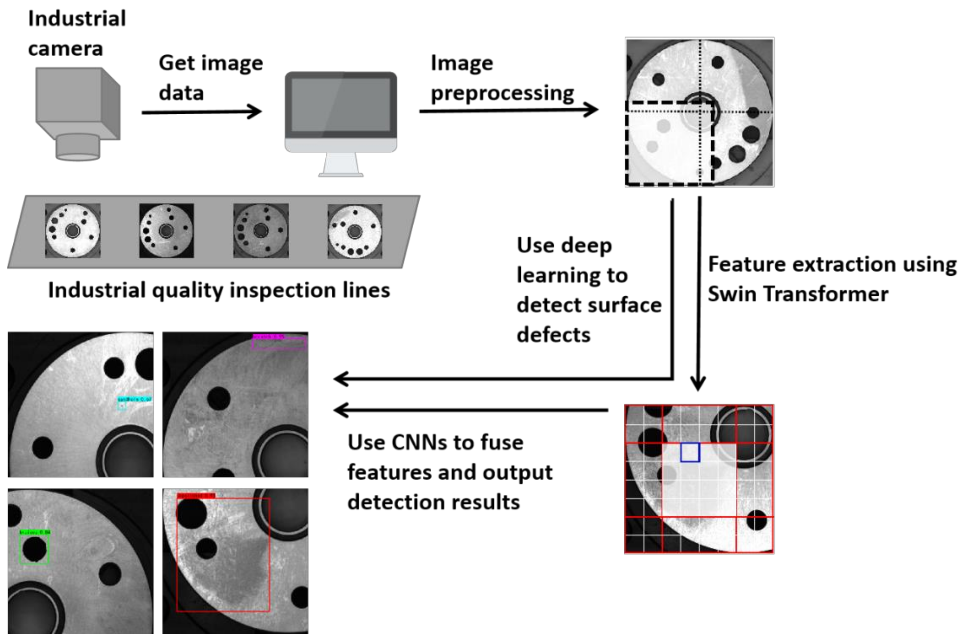This allows the model to focus more on those defects that are difficult to detect, which is helpful for the surface defect detection task [18]. The proposed model outperforms mainstream target detection algorithms on our private dataset of flange surface defects task and outperforms most existing models on public datasets of steel surface defects. The diagram of the process for detecting defects in flanges using our method is shown in Figure 1.

2. Method

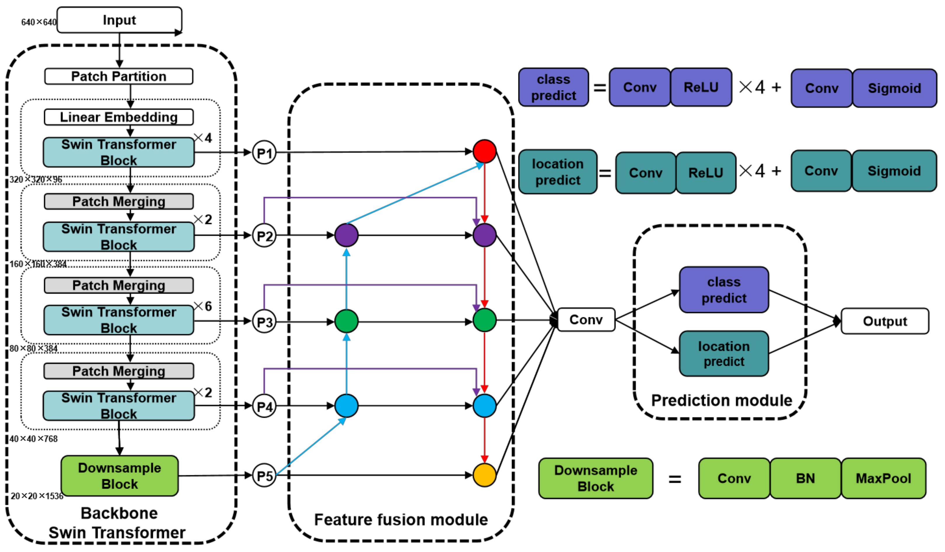
The overall architecture of the proposed method is shown in the Figure 2, containing the backbone, feature fusion module and prediction module. The images are input into the patch partition in a Swin transformer to be split into non-overlapping patches. The feature of each patch is set to the concatenation of the original pixel RGB values. The size of each patch is 4 × 4, resulting in a feature dimension of each patch of 48 (4 × 4 × 3). The original features are adjusted to 96 after passing through the linear embedding layer. Then, the Swin transformer blocks are used for self-attentive computation and the first scale features are output. The patch merging layers are responsible for reducing the number of tokens, which can produce feature representations at different scales. A patch merging layer and several Swin transformer blocks are used as a combination to perform feature extraction. Three such combinations are present, and they can produce three layers of features at different scales. The deepest feature of the Swin transformer goes through a downsample block and outputs the fifth scale feature. The features of these five scales are input into the neck of the network for weighted feature fusion, after which the outputs of the five scales are fed into the detection head of the network for category and location prediction to obtain the final detection results.

2.1. Backbone

As shown in Figure 2, after an image of size H × W × 3 is input into the backbone, it is first processed by patch partition to transform the image into 4 × 4 × 3 patches. The dimensions are converted from 48 to 96 by linear embedding. Unlike the original Swin transformer tiny, we input the data into four Swin transformer blocks for the first self-attentive computation. Many fine-grained features are present in the shallow layer with higher resolution, and we expect the network to learn these features in the shallow layer, benefiting the detection of surface defects on small targets. The obtained output P1 is input into the neck and input into patch merging for scale transformation. The transformed features are input to the Swin transformer block for self-attentive calculation. Patch merging with several Swin transformer blocks is configured as a combination of three groups, where the number of Swin transformer blocks are 2, 6 and 2. These blocks output P2, P3 and P4, respectively, to the neck of the network. P4 is downsampled by a simple structure consisting of convolution, batch normalization and Maxpool to obtain the output P5, helping enhance the perceptual field of the original Swin transformer.

2.1.1. Patch Merging

Given that the self-attentive computation does not change the size and dimension of the features, and we want to get hierarchical features in the Swin transformer as in CNNs, we need to add a patch merging layer. The schematic diagram of patch merging is shown in Figure 3, where the first operation is to sample the incoming data at one point intervals and patch the sampled results in a dimension so that the dimension of the feature is expanded by four times and the size is reduced to one half of the original size. The second operation converts a feature of dimension 4C to 2C using a convolutional operation with a kernel size of 1 × 1. The patch merging operation consisting of the first operation and the second operation can achieve a hierarchy of features, which is important for target detection.

2.1.2. Swin Transformer Block

The flow chart of a Swin transformer block is shown in Figure 4, where $f^{i-1}$ is the input and $f^{i+1}$ is the output. LN stands for layer normalization, MLP stands for multilayer perceptron, W-MSA stands for windows multi-head self-attention and SW-MSA stands for shifted windows multi-head self-attention. These modules are used alternately in the Swin transformer block, and the mathematical expression can be expressed as

$${\widehat{f}}^i=W-MSA\left(LN\left(f^{i-1}\right)\right)+f^{i-1}$$

$$f^i=MLP\left(LN\left({\widehat{f}}^i\right)\right)+{\widehat{f}}^i$$

$${\widehat{f}}^{i+1}=SW-MSA\left(LN\left(f^i\right)\right)+f^i$$

$$f^{i+1}=MLP\left(LN\left({\widehat{f}}^{i+1}\right)\right)+{\widehat{f}}^{i+1}$$

(1)

W-MSA is more efficient than global multi-head self-attention, and it enables dense prediction of high-resolution images. Given that its self-attention computation is performed within a local window, assuming here that N × N patches are within each window and the size of each patch is H × W, the computational complexity of global multi-head self-attention is

$$\mathsf{\Omega }\left(\mathrm{MSA}\right)=4{\mathrm{HWC}}^2+2{\left(\mathrm{HW}\right)}^2$$

(2)

The computational complexity of shifted windows multi-head self-attention is

$$\mathsf{\Omega }\left(\mathrm{W}-\mathrm{MSA}\right)=4{\mathrm{HWC}}^2+2{\mathrm{N}}^2\mathrm{HW}\mathrm{C}$$

(3)

where C is the channel of the feature. The computational complexity is quadratic to HW when using MSA for self-attentive computation, while it is linear to HW when using W-MSA, making W-MSA capable of affordable computation for large HW.

Given that the windows separated by W-MSA are fixed, no information exchange occurs between different windows, which will bring adverse effects to the modelling ability of the model. Therefore, SW-MSA is introduced, which enables information communication between different windows by a simple window shift. As shown in Figure 3, W-MSA and SW-MSA are used alternately in the Swin transformer block so that the model can perform self-attentive calculations and perform best on large-scale images. The schematic diagrams of MSA, W-MSA and SW-MSA are shown in Figure 5.

Each non-overlap window W of W-MSA can be expressed as

$$\mathrm{Q}={\mathrm{WP}}_{\mathrm{Q}},\mathrm{K}={\mathrm{XP}}_{\mathrm{K}},\mathrm{V}={\mathrm{XP}}_{\mathrm{V}}$$

(4)

The shared projection matrix on all windows is ${\mathrm{P}}_{\mathrm{Q}}$, ${\mathrm{P}}_{\mathrm{K}}$, ${\mathrm{P}}_{\mathrm{V}}$. Q, K and V denote query, key and value, respectively, $\mathrm{B}\in {\mathrm{R}}^{{\mathrm{N}}^2\times {\mathrm{N}}^2}$indicating relative position bias. d is the dimension of query/key. They are used to calculate the self-attentive mechanism in one window, which can be formulated as

$$\mathrm{Attention}\left(\mathrm{Q},\mathrm{K},\mathrm{V}\right)=\mathrm{SoftMax}\left({\mathrm{QK}}^{\mathrm{T}}/\sqrt{\mathrm{d}}+\mathrm{B}\right)\mathrm{V}$$

(5)

2.2. Feature Fusion Module

After the input data passes through several layers of patch merging and Swin transformer block, the feature extraction module will extract richer semantic information and obtain more channels, but the size of the data will also be reduced and some fine-grained information will disappear, resulting in the inability to extract these features. By fusing the features of different layers, the shallow features can be made to acquire the deep semantic information and the deep network to acquire the shallow fine-grained information to improve the detection capability of the model [19]. We use BiFPN as the feature fusion part, which is structured as shown in the neck part in Figure 2. The blue arrows represent the paths from the deep features to the shallow layers, which are responsible for transmitting semantic information. The red arrows represent the transfer of texture information from shallow to deep layers. The purple arrow transfers the raw features extracted by the backbone to the final output, which allows the model to fuse more features with minimal computational cost.

A total of five different scales of features are output from the backbone, where $P_1,P_2,P_3$ and $P_4$ are the features extracted by the Swin transformer block. $P_5$ is obtained from downsampling on the basis of $P_4$. Adding $P_5$ consumes only a small amount of computational resources, but it can improve the detection performance of the model for large-scale targets. For the one-way path input nodes $\left(P_1, P_5\right)$, their contribution to feature fusion is small, thereby simplifying its fusion process. Let the nodes with bi-directional paths (bottom-up and top-down) be a feature network layer (e.g., $P_2, P_3$,$P_4$). For the feature network layer, a variety of weighted feature fusion processes is taken.

For example, its feature fusion process is shown in Equation (6), where ${\mathsf{\omega }}_{\mathrm{i}}$ represent the weights, ${\mathrm{I}}_{\mathrm{i}}$ represent the features and $\mathsf{\epsilon }$ is a constant to ensure a stable value.

The $P_4^{in}$ features from the backbone input are weighted, $P_5^{in}$ is upsampled to have the same size as $P_4^{in}$ and then weighted, and the two are summed and convolved to obtain $P_4^{td}$. We weight $P_4^{in}$, weight $P_4^{td}$ and weight $P_3^{out}$ after downsampling it to the same size as $P_4^{td}$, and compute $P_4^{out}$ by convolution after summing the total of the three. $P_4^{out}$ performs multiple feature fusions and these are not simply summed, but a weighted summation is performed to enhance the effect of important features on the fusion results. The features are weighted using fast normalised fusion, which is calculated in Equations (7) and (8). Using the Relu activation function ensures that each ${\mathsf{\omega }}_{\mathrm{i}}\ge 0$ and $\mathsf{\epsilon }$ = 0.0001 ensures stable values. BiFPN integrates fast normalized fusion with bi-directional cross-scale connectivity to efficiently fuse features from different scales.

$$\mathrm{O}={{\displaystyle \sum }}_{\mathrm{i}}\frac{{\mathsf{\omega }}_{\mathrm{i}}}{\mathsf{\epsilon }+{{\displaystyle \sum }}_{\mathrm{j}}{\mathsf{\omega }}_{\mathrm{j}}}·{\mathrm{I}}_{\mathrm{i}}$$

(6)

$$P_4^{td}=Conv\left(\frac{{\mathsf{\omega }}_1·P_4^{in}+{\mathsf{\omega }}_2·\mathrm{UpSample}\left(P_5^{in}\right)}{{\mathsf{\omega }}_1+{\mathsf{\omega }}_2+\mathsf{\epsilon }}\right)$$

(7)

$$P_4^{out}=Conv\left(\frac{{\mathsf{\omega }}_1^{\prime }·P_4^{in}+{\mathsf{\omega }}_2^{\prime }·P_4^{td}+{\mathsf{\omega }}_3^{\prime }·\mathrm{DownSample}\left(P_3^{out}\right)}{{\mathsf{\omega }}_1^{\prime }+{\mathsf{\omega }}_2^{\prime }+{\mathsf{\omega }}_3^{\prime }+\mathsf{\epsilon }}\right)$$

(8)

2.3. Prediction Module

The prediction module is shared by five scale outputs, which is based on the anchor box for detection. The five scales of features output by the feature fusion side will first adjust the dimensionality to 256 uniformly and then will be sent to the class predict block and location predict block to predict the fused features. From Figure 2, which shows their structure, Weight × Height × Number of classes × Anchor is output from the class predict block. Weight × Height × 4 × Anchor is output from the location predict block, where 4 indicates the prediction of the target’s location. Among them, three sizes of anchor box {$2^0,2^{1/3},2^{2/3}$} are used, configured with three aspect ratios {1:2,1:1,2:1}. Each size of the feature output is assigned nine anchor boxes. We share the head module for the prediction of the results because it can reduce the number of parameters and can effectively alleviate the overfitting and improve the accuracy of the detection.

2.4. Loss Function

The two-stage target detection algorithm first calculates the region proposal and then performs target detection in the area where the target may exist. Given that the one-stage target detection algorithm does not have the process of region proposal, this will lead to a situation in which the foreground and background are extremely unbalanced. In addition, a large number of small target defects are found in the surface defects of industrial parts, which are prone to many negative samples during detection. When the number of negative samples is high to a certain extent, it will weaken the effect of those important samples on training. Therefore, we choose focal loss [20] as the loss function to overcome this problem.

The standard cross-entropy (CE) loss can be expressed as

$$\mathrm{CE}\left(\mathrm{p},\mathrm{y}\right)=\left\{\begin{array}{c}-\log \left(\mathrm{p}\right) \mathrm{if} \mathrm{y}=1\\ -\log \left(1-\mathrm{p}\right) \mathrm{otherwise}\end{array}\right.$$

(9)

ground-truth class is represented by $\mathrm{y}\in \left\{\pm 1\right\} \mathrm{and} \mathrm{p}\in \left[0,1\right]$ is the probability value of the model predicting y = 1.

${\mathrm{p}}_{\mathrm{t}}$ is defined as the following equation

$${\mathrm{p}}_{\mathrm{t}}=\left\{\begin{array}{c}\mathrm{p} \mathrm{if} \mathrm{y}=1\\ 1-\mathrm{p} \mathrm{otherwise}\end{array}\right.$$

(10)

Then, the CE loss can be expressed as

$$\mathrm{CE}\left(\mathrm{p},\mathrm{y}\right)= \mathrm{CE}\left({\mathrm{p}}_{\mathrm{t}}\right)=-\log \left({\mathrm{p}}_{\mathrm{t}}\right)$$

(11)

Generally, adding weighting factors is a solution to the class imbalance problem. We treat balance CE loss as the baseline of focal loss, which can be expressed as

$$\mathrm{CE}\left({\mathrm{p}}_{\mathrm{t}}\right)=-{\mathsf{\alpha }}_{\mathrm{t}}\log \left({\mathrm{p}}_{\mathrm{t}}\right)$$

(12)

$\mathsf{\alpha }$-balance CE loss weights the importance of positive and negative samples. The focal loss adds a moderator to the CE loss, which differentiates the difficulty of the sample classification so that the model focuses on the difficult samples. Focal loss can be expressed as

$$\mathrm{FL}\left({\mathrm{p}}_{\mathrm{t}}\right)=-{\mathsf{\alpha }}_{\mathrm{t}}{\left(1-{\mathrm{p}}_{\mathrm{t}}\right)}^{\mathsf{\gamma }}\log \left({\mathrm{p}}_{\mathrm{t}}\right)$$

(13)

manner where ${\left(1-{\mathrm{p}}_{\mathrm{t}}\right)}^{\mathsf{\gamma }}$ is the modulation factor, $\mathsf{\gamma }$ is the focusing parameter that adjusts the rate at which easily classified samples are down-weighted. In our experiments, $\mathsf{\gamma }$ is set to 2, which is the same as in [20].

3. Experiment

3.1. Dataset

The original flange surface defect data was collected by Daheng MER-500 industrial camera, and 200 pictures with a resolution of 2592 × 1944 were collected under three different lighting conditions. If the large size of the original map is directly downsampled and then fed into the model, it will lead to the disappearance of small target features, which is unfavorable for the feature extraction of the model and will directly lead to the missing detection of small target defects. Therefore, before labelling the data, some pre-processing of the original data is needed.

As shown in Figure 6a, we first crop the redundant background in the image to keep the grey area and then crop a pair of images into four copies according to the overlap rate of 15%, and the size of each image is 1040 × 1040. On this basis, downsampling is performed to adjust the size to 640 × 640 for input to the model.

There are two reasons for processing the data as described above: (1) If the 2592 × 1944 pixel image is directly adjusted to a 640 × 640 pixel image, it will lead to the disappearance of fine-grained features, which is negative for the model to fit the flange surface defects. (2) Cropping the image according to a 15% overlap rate will ensure the integrity of the medium-sized defect bruises and enable the model to learn its features better. If the pictures are not cropped according to the certain overlap rate, it will lead to the learning targets being separated, which is disadvantageous for the model to fit the data [21].

After pre-processing the original image data, we annotated the processed images according to the criteria of the VOC dataset, and the annotation of four different defects is shown in Figure 6b.

We use a mixture of rotation, translation, flip and contrast to augment the data, expanding the amount of data to 10 times the original size. Notably, we have used some advanced data enhancement methods such as mosaic, cutmix and cutout for our experiments and found that these methods are not suitable for surface defect data enhancement. Given that many small targets are already present in the original data, further stitching operations will make extracting the features of the small targets difficult for the model. By contrast, using these methods generates a certain amount of redundant gradient information, which is detrimental to the training of the model. After suitable data enhancement, 80% of the data is used for model training, 10% for validation and 10% for testing.

3.2. Evaluation

We mainly use mAP, frames per second (FPS), parameters, and FLOPs as the main evaluation metrics of the model [22]. mAP is the metric used to evaluate multi-category detection, which is the mean value of AP (average precision). AP is the area under the precision-recall curve for a particular class. Precision refers to the proportion of correctly predicted ‘TRUE’ samples out of all predicted ‘TRUE’ samples, and it is calculated as

$$\mathrm{P}=\frac{\mathrm{TP}}{\mathrm{TP}+\mathrm{FP}}\in \left[0,1\right]$$

(14)

Recall refers to the proportion of correctly predicted ‘TRUE’ samples out of all predicted ‘TRUE’ samples, and it is calculated as

$$\mathrm{R}=\frac{\mathrm{TP}}{\mathrm{TP}+\mathrm{FN}}\in \left[0,1\right]$$

(15)

The AP is calculated as

$${\mathrm{AP}}_{\mathrm{i}}={{\displaystyle \int }}_0^1{\mathrm{P}}_{\mathrm{i}}\left({\mathrm{R}}_{\mathrm{i}}\right)d{R}_i$$

(16)

AP is the average value of AP under different IoU (IoU from 0.50 to 0.95 where the step is 0.05), and the IoU is calculated as in (16), where X represents the detection area and Y represents the real area of the target. The larger the IoU, the more accurate the detection result.

$$\mathrm{IoU}=\frac{\mathrm{X}\cap \mathrm{Y}}{\mathrm{X}\cup \mathrm{Y}}$$

(17)

The equation for mAP is calculated as

$$\mathrm{mAP}=\frac{{{\displaystyle \sum }}_1^{\mathrm{n}}{\mathrm{AP}}_{\mathrm{i}}}{\mathrm{n}}$$

(18)

The closer the mAP is to 1, the better the detection of the model.

FPS represents how many images the model can process per second, and it is the most intuitive indicator of the detection speed. The higher the FPS, the faster the detection speed of the model.

The FPS is calculated as

$$\mathrm{FPS}=\frac{1}{\mathrm{t}}$$

(19)

where t represents the time in units of seconds to detect an image.

Floating point operations (FLOPs) represents the computational volume of the model. Parameters represent the complexity of the model. Smaller values of these two indicators indicate a more streamlined model.

3.3. Training Strategy and Experimental Environment

Before training the surface defect data, we load the weights of the backbone feature network after pre-training on the image Net1k [23] dataset, allowing the network to converge faster and preventing overfitting [24]. The pre-training strategy is as follows: optimizer is SGD, learning rate is 0.02, momentum is 0.9, weight decay is 0.0001 and epoch is set to 300 [25].

For the flange surface defect data, our training strategy is as follows: optimizer is SGD [26] (learning rate is 0.002, momentum is 0.9 and weight decay is 0.0001). Batch size is set to 24 and epoch is set to 100.

Our experimental environment is as follows: Ubuntu 20.04.4, Intel Xeon Silver 4210 CPU, NVIDIA A10*2 GPU, 64 GB RAM, Python version 3.7, Torch version 1.9.0 and CUDA version 11.1.

3.4. Comparison Method

We choose the most advanced one-stage detection algorithms YOLOX [27] and RetinaNet and the most classical two-stage detection algorithm, Faster-RCNN [28], as the methods for comparison experiments. We use CSPdarknet-L as the backbone of YOLOX and resnet50 [29] as the backbone of RetinaNet and Faster-RCNN, which have similar FLOPs and parameters as the Swin transformer tiny.

4. Experimental Results and Discussion

4.1. Detection Results

Table 1. Performance of different models on the flange surface defect dataset.

Method	Sand_Hole	Unpolished	Scratch	Bruises	mAP
YOLOX-L	0.518	0.834	0.803	0.701	0.714
Retinanet	0.582	0.891	0.837	0.75	0.765
Faster-RCNN	0.567	0.878	0.812	0.719	0.744
Our Method	0.67	0.968	0.934	0.892	0.866

shows the performance of different models on the flange surface defect dataset we constructed. mAP of YOLOX-L, RetinaNet-Resnet50 and Faster-RCNN-Resnet50 are 0.714, 0.765 and 0.744, respectively. Similar to the description of [20], RetinaNet, as a one-stage detection algorithm, outperforms the two-stage detection algorithm Faster-RCNN. Our method achieves the optimal result among all methods with a mAP of 0.866. In Figure 7, the detection results for the flange surface defect data are shown, where a to d are scratched, sand holes, bruises and unpolished, respectively.

4.2. Efficiency Analysis

We compared the parameters, FLOPs and FPS of different methods separately to analyze their efficiency. The experimental results are shown in

Table 2. Efficiency analysis.

Method	Parameters	FLOPs	FPS
YOLOX-L	54.15	77.67	27.1
Retinanet	36.21	82.57	35.8
Faster-RCNN	41.15	91.03	37.4
Our Method	37.1	84.9	23.5

. The parameter number of our method is slightly higher than that of RetinaNet, which is 37.1 M, and the FLOPs are 84.9, which is lower than that of Faster-RCNN. Its FPS on our GPU is 23.5, and only 0.042 s are needed to detect each pair of images, which can achieve the requirement of real-time detection.

4.3. Ablation Experiments

We performed some ablation experiments on our model to demonstrate the effectiveness of the network we designed. We replaced the backbone with resnet50, the feature fusion part with PANET [30] and the loss function with cross-entropy loss, respectively, and compared their performance on the flange surface defect dataset. The results are shown in

Table 3. Ablation experiments.

Method	mAP	Parameter	FLOPs	FPS
Ourmethod	0.866	37.1	84.9	23.5
Resnet50+bifpn+focalloss	0.759	36.9	83.1	35.3
SwinT+bifpn+crossentropyloss	0.731	37.1	84.9	23.5
SwinT+pafpn+focalloss	0.837	38.2	86.3	22.7

. Our method achieves the highest mAP. The parameter and FLOPs are only slightly higher than the method using resnet50 as a backbone. The FPS is 10 lower compared with the method using resnet50 as a backbone but gains a 10.7% improvement in mAP, which we think is a worthwhile compromise.

4.4. Extensibility Analysis

We conducted experiments on a common dataset, Steel Surface Defects [31] (NEU-DET), to demonstrate that our proposed defect detection method works well not only for flange surface defect detection but also in other defect detection areas. This dataset consists of a total of 1800 images with a pixel size of 192 × 192 for six common steel surface defects. We divide 80% data for training, 10% data for validation and 10% data for testing. For NEU-DET, we adjust the batch size to 64 because it has a data size of 192 × 192 pixels, giving our GPU the ability to train more samples at once and also to fit these data better.

In the comparison experiments, we added other researchers’ methods for comparison. Lv et al. [32] used a method based on Single Shot MultiBox Detector for defect detection. Kou et al. [33]. improved YOLOV3 for defect detection.

The experimental results are shown in

Table 4. Performance of different models on the steel surface defect dataset.

Method	Crazing	Inclusion	Patches	Pitted_Surface	Rolled_in_Scale	Scratches	mAP
YOLOX	0.322	0.428	0.695	0.749	0.408	0.658	0.543
Retinanet	0.331	0.574	0.708	0.765	0.41	0.693	0.592
Faster-RCNN	0.377	0.494	0.714	0.814	0.556	0.478	0.572
Lv et al.	0.417	0.763	0.863	0.851	0.581	0.856	0.724
Kou et al.	0.389	0.737	0.935	0.748	0.607	0.914	0.722
Our Method	0.465	0.842	0.972	0.843	0.641	0.926	0.781

. Although our model is constructed for flange surface defects, our method outperforms not only the classical target detection algorithms but also the defect detection algorithms designed by other researchers on NEU-DET. This shows that the Swin transformer can effectively extract defect features and confirms the competitiveness of our method. The detection results based on NEU-DET are shown in Figure 8, where a to f are crazing, inclusion, patches, pitted surface, rolled in scale and scratches, respectively.

5. Conclusions

This paper applies a Swin transformer combined with CNNs approach to surface defect detection tasks in industry. We demonstrate experimentally that the Swin transformer has a stronger feature extraction capability compared with CNNs in surface defect detection. We simply improve the Swin transformer’s structure and apply it to a single-stage target detection algorithm that we design to fully exploit its advantages. We have improved the commonly used feature pyramid network by using a weighted feature pyramid network that fuses five scaled features output from the Swin transformer. Focal loss can focus the model more on difficult-to-detect defects objects. Shared prediction module prevents overfitting while effectively reducing the model parameters. Combining the above methods, we have designed a novel and high performance one stage defect detection algorithm.

In our constructed dataset, our method shows a great advantage over the CNN-based method on mAP, while it possesses a satisfactory detection speed. In addition, we analyzed the performance of our method on NEU-DET dataset. The experimental results show that our method is not only applicable to specific problems, but also has good scalability on other problems. In the future, we look forward to applying Swin transformers to other industrial applications.