1. Introduction
With the advancement of technology, intelligent robots have gradually entered people’s lives. Normal work of intelligent robots is inseparable from their positioning. Usually, the positioning problem of a robot is solved by the GNSS positioning system [
1,
2]. However, in scenarios such as weak satellite signals or signals indoors, the GNSS system alone cannot achieve high-precision positioning. In 2020, the China Association for Science and Technology pointed out that achieving high-precision positioning and navigation when satellite signals are unavailable has become an urgent engineering and technical problem to be solved. To complete positioning in an environment where a satellite signal is rejected is usually to use sensors such as the wheel speedometer and inertial navigation to calculate the position of the robot by using its motion information [
3]. However, the wheel speedometer has high requirements for the model accuracy of the robot, and robot mileage estimation based on the wheel speedometer cannot guarantee high accuracy due to possible road surface unevenness and slippage during the robot’s movement. Although inertial navigation is not affected by the model or the environment, drift of data is amplified in the process of quadratic integration and cannot be corrected independently. Based on the reasons above, the multi-sensor fusion positioning method has gradually entered the field of vision. Commonly used sensors include monocular, stereo, RGB-D cameras, lidar, millimeter-wave radar, UWB (ultra-wideband) [
4], etc. Using these sensors, multi-sensor positioning systems such as VO (visual odometry), VIO (visual inertial odometry) and LIO (lidar inertial odometry) have been developed. Because of adoption of multi-sensor fusion methods supplemented by various filtering algorithms, data errors of the sensors themselves are eliminated and positioning accuracy is greatly improved.
SLAM is a means of using a variety of sensors to achieve high-precision, real-time positioning and mapping for robot navigation [
5]. At first, SLAM was mainly used in the positioning of small indoor robots. The indoor environment could be mapped with 2D single-line lidar and analyzed with post-processing. Today, SLAM is able to perform 3D analyses of the surrounding environment, and implementation methods are mainly divided into visual SLAM and lidar SLAM [
6]. Visual SLAM, which is undergoing rapid development, relies on the advancement of image-processing technology, with mature visual feature points and descriptor extraction methods as well as many vision-based deep neural networks. Among them, the ORB (oriented FAST and rotated BRIEF)-SLAM3 [
7] algorithm, which is suitable for monocular, binocular and RGB-D cameras for back-end mileage estimation using cluster adjustment, has become the master of visual SLAM algorithms and has been widely used for reference by other visual SLAM algorithms. In terms of using natural language processing, Rosinol et al. summarized previous experience and established the Kimera [
8] open-source SLAM library based on the DBoW2 [
9] word bag library. McCormac combined semantic information and convolutional neural networks to propose the SemanticFusion [
10] algorithm, which performed well on the NYUv2 [
11] dataset and maintained a running speed of 25 Hz. Because lidar SLAM has experienced the process of developing from 2D to 3D, Google open-sourced Cartographer [
12], an algorithm based on graph optimization for 2D/3D, in 2016. This algorithm does not include PCL, g2o, etc., which are huge code bases and have simple architecture suitable for lightweight and low-cost robots such as home robots. Zhang et al. proposed the LOAM [
13] algorithm, in which only single-line lidar was used to realize the mapping of the 3D environment, in 2014. It is still widely admired today and maintains the third position on the rank of dataset KITTI (Karlsruhe Institute of Technology and Toyota Technological Institute) [
14]. Its framework is used by many researchers as a basis for building algorithms. For example, Lego-LOAM [
15] is suitable for lightweight robots, I-LOAM [
16] provides loop-closure detection and echo-accuracy information and SA-LOAM [
17] provides semantic information. Ding et al. proposed the Deepmapping [
18] algorithm using deep neural networks combined with traditional algorithms, which made mapping more accurate but sacrificed real-time performance of the algorithm.
Although the SLAM algorithm has been successfully applied in clear situations and simple scenes, odometer estimation accuracy is reduced in complex scenes with many dynamic objects. Mainstream odometer estimation method is based on feature point matching within static world assumption [
19]; feature points extracted from dynamic objects are treated as static feature points. These dynamic points influence the matching result. Removing the influence of dynamic objects has become the goal of current SLAM algorithm development [
20,
21].
The most popular method of removing influence caused by dynamic objects is identifying and marking dynamic objects and removing feature points on marked parts [
22,
23,
24]. There are mainly two methods to identify dynamic objects: traditional methods based on geometric information and neural network methods based on semantic information. These methods have different degrees of improvement for lidar SLAM.
In 2020, Yangzi Cong et al. used UGV as an experimental platform, first filtering out the ground point cloud, then roughly segmenting suspected dynamic objects using traditional clustering methods, using Kalman filter to identify and track suspected point clouds and using probabilistic map assistance to complete tracking and mapping [
25]. Compared with Lego-LOAM, which is applied to similar unmanned platforms but does not remove dynamic objects, the result of Yang’s method was better. However, compared with the algorithm that uses semantic information for dynamic object processing, effect of dynamic object recognition was worse, and positioning accuracy was also lower. In 2021, Feiya Li et al. proposed a method to establish an initial vehicle model based on shape characteristics of the vehicle, and constructed and removed sparse points based on the boundary line formed by residual points [
26]. Identification and tracking of vehicles were completed through calculation of confidence level of the vehicle model and adaptive threshold, which provided a new idea for dealing with dynamic objects. In 2019, on the basis of Suma, Xieyuanli Chen et al. used the RangeNet++ network to semantically label point clouds and proposed the Suma++ algorithm [
27]. For each row of point cloud semantic segmentation, the same semantics were searched and filled in the whole. A dynamic information removal module was added to the Suma framework, and map information was used to identify the dynamic point cloud of this frame. At the same time, semantic constraints were added to the ICP(Iterative Closet Point) algorithm to improve robustness of the algorithm with singular values. However, the algorithm could not identify dynamic objects in the first observation, and required two frames of information for comparison. In 2021, Shitong Du et al. fused semantic information to propose S-ALOAM [
28], labeling dynamic objects in the preprocessing stage and removing dynamic objects and singularities. Feature extraction was performed on point clusters with the same semantic label according to geometric rules. The odometer node roughly estimated the motion matrix and performed transformation correction. At the mapping node, dynamic objects were eliminated again, with semantic constraints, to complete laser point cloud mapping. However, it took a lot of time to recognize through semantic tags, which affected the real-time performance of the algorithm. In summary, processing dynamic objects can improve positioning accuracy of the SLAM algorithm and improve the mapping effect. However, whether it is the traditional method or the method using the neural network, it is difficult to maintain a fast running speed while ensuring a high recognition rate of dynamic objects. It is necessary to propose a new SLAM algorithm that can not only ensure the recognition rate of dynamic objects to ensure positioning accuracy, but also ensure running speed of the algorithm to ensure real-time performance of the algorithm.
2. Materials and Methods
In order to solve the problem of accuracy of odometer motion estimation decrease due to the large number of pedestrians and vehicles in the city, and at the same time to ensure real-time performance of the algorithm, this paper proposes a lidar SLAM algorithm in dynamic scenes. It realizes the labeling of ground point cloud data, removes the point cloud of dynamic objects and repairs the removed blank area according to the adjacent point cloud. Inertial navigation data was introduced to eliminate motion distortion of original point cloud data and, at the same time, considering the difference in feature types of the point cloud in ground and non-ground areas, classification features were extracted and features were matched according to category in the odometer estimation stage. In the motion estimation stage, a weight factor was introduced to reduce the influence of possible noise feature points, and motion trajectory estimation results were re-corrected in the mapping stage to improve accuracy of the algorithm.
The main flow of the algorithm was as
Figure 1:
In this paper, the inertial navigation coordinate system of the starting position of robot motion was selected as the world coordinate system. In the solution process, the lidar coordinate system was set as the {L} coordinate system, the inertial navigation coordinate system was set as the {B} coordinate system and the world coordinate system was set as the {W} coordinate system. When movement started, .
2.1. Distortion Removal
The lidar point cloud acquisition process took a long time for each frame and the point cloud was distorted due to movement of the robot itself during the acquisition process. Using inertial navigation data helped correct for nonlinear distortions that occurred during acquisition. Since acquisition frequency of inertial navigation was much higher than that of lidar, a circular buffer was used to store inertial navigation data, and data of the two sensors were matched according to the timestamp. There were no inertial navigation data at the corresponding time of some lidar points, and the motion state of these lidar points was obtained by linear interpolation of the inertial navigation motion state according to acquisition time of these lidar points. Acquisition time
could be calculated from number of lidar lines
and horizontal angles
.
where
represents the number of the bottommost line of lidar,
represents the number of the topmost line of lidar,
represents the starting timestamp of this frame,
and
represent time parameters of lidar and
represents horizontal angle resolution of lidar.
The number of lidar lines and horizontal angles of lidar points could be calculated from point coordinate
, the topmost vertical angle
and the bottommost vertical angle
.
The state of motion was calculated through integration of acceleration and angular acceleration provided by inertial navigation data. Assuming that the robot moved at a uniform speed during the point cloud acquisition process, motion distortion
in {W} was calculated according to the difference between the estimated state
in {W} at current moment
as well as the uniform motion estimation result, which was calculated from the beginning of the frame
to the current moment with estimated state
in {W} and speed at the beginning of this frame
in {W}.
The nonlinear motion distortion was eliminated through subtraction of the respective distortion from the lidar point.
2.2. Ground Labeling
The ground point cloud was identified to separate objects from the background, which facilitated feature extraction. Lidar points were divided into different grids
according to the X and Y coordinates, lidar scanning range
and grid resolution
,
The point cloud was projected to the XOY plane of the world coordinate system, where function ‘floor’ means rounding down of the input.
For each grid
, it was necessary to calculate average height
of all lidar points’ height
in the grid and height difference
between the highest point
and the lowest point
, then establish an elevation map mean (mean map) and an elevation map min-max (difference map).
where function
calculates the total number of lidar points.
For each grid in the mean map, it was necessary to calculate gradient in the four neighborhoods and select the maximum gradient as the gradient of the grid. The gradient and of every grid were compared with the threshold and . A grid where both parameters were greater than threshold was identified as an object; where both were less, it was identified as a ground grid. Other grids were pended.
Through the breadth-first search (BFS) algorithm, the four neighborhoods of the ground grid were searched for clustering and multiple ground planes were obtained after clustering. The plane with the largest area among the multiple planes was identified as the ground. The average height difference between other planes and the ground was calculated and difference was compared with the threshold . A grid with a height difference from the ground that was less than the threshold was identified as ground and a grid with a height difference from the ground that was greater than the threshold was identified as ‘other planes.’
The undetermined grid was traversed and voxelized. First, the undetermined grid was divided into small grids with smaller resolutions: and . Vertical bars were established within each small grid according to the highest point and the lowest point of the small grid; the vertical bars were divided into voxels using voxel resolution . Voxels that contained points were retained and those that did not contain points were removed. Voxels were clustered and the group of voxels with the lowest height was taken as the ground part of the grid. In comparison of these low-voxel groups with the determined ground grid, the voxel group where mean heights were within the range of above or below ground height could be identified as ground voxel groups, and points contained in the voxel groups were identified for the ground point cloud.
2.3. Dynamics Removal
According to number of lines
, horizontal angle
and coordinates, the point cloud was projected into the range image according to Equation (6).
Since the intensity of some lidar points was lower than the receiving threshold, some information could not be received, resulting in missing point clouds. Each missing point cloud was classified and filled in and its range given value; when the range difference between the two boundary points or the sequence number difference was small enough, the linear interpolation value of boundary range was used as a range to fill in missing point positions. After filling was completed, Equation (6) was used to calculate its three-dimensional coordinates inversely. Then the backward difference was used to calculate the first derivative of the range of point , where , were, respectively, the range of points and . Forward difference was used to calculate the second derivative of the range of point , where is the range of points .
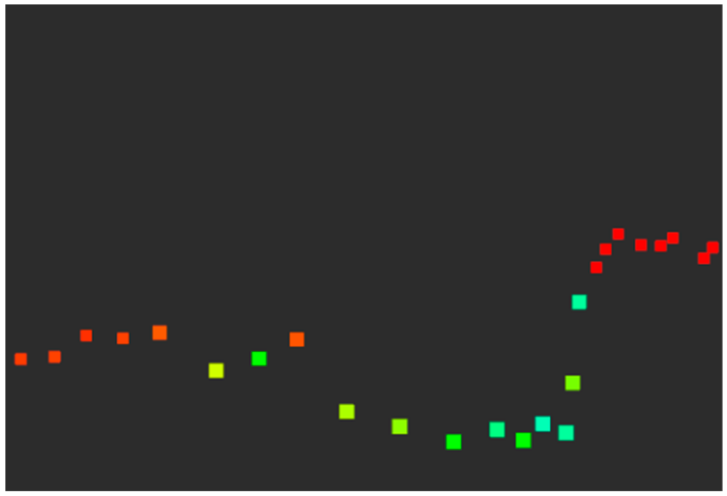
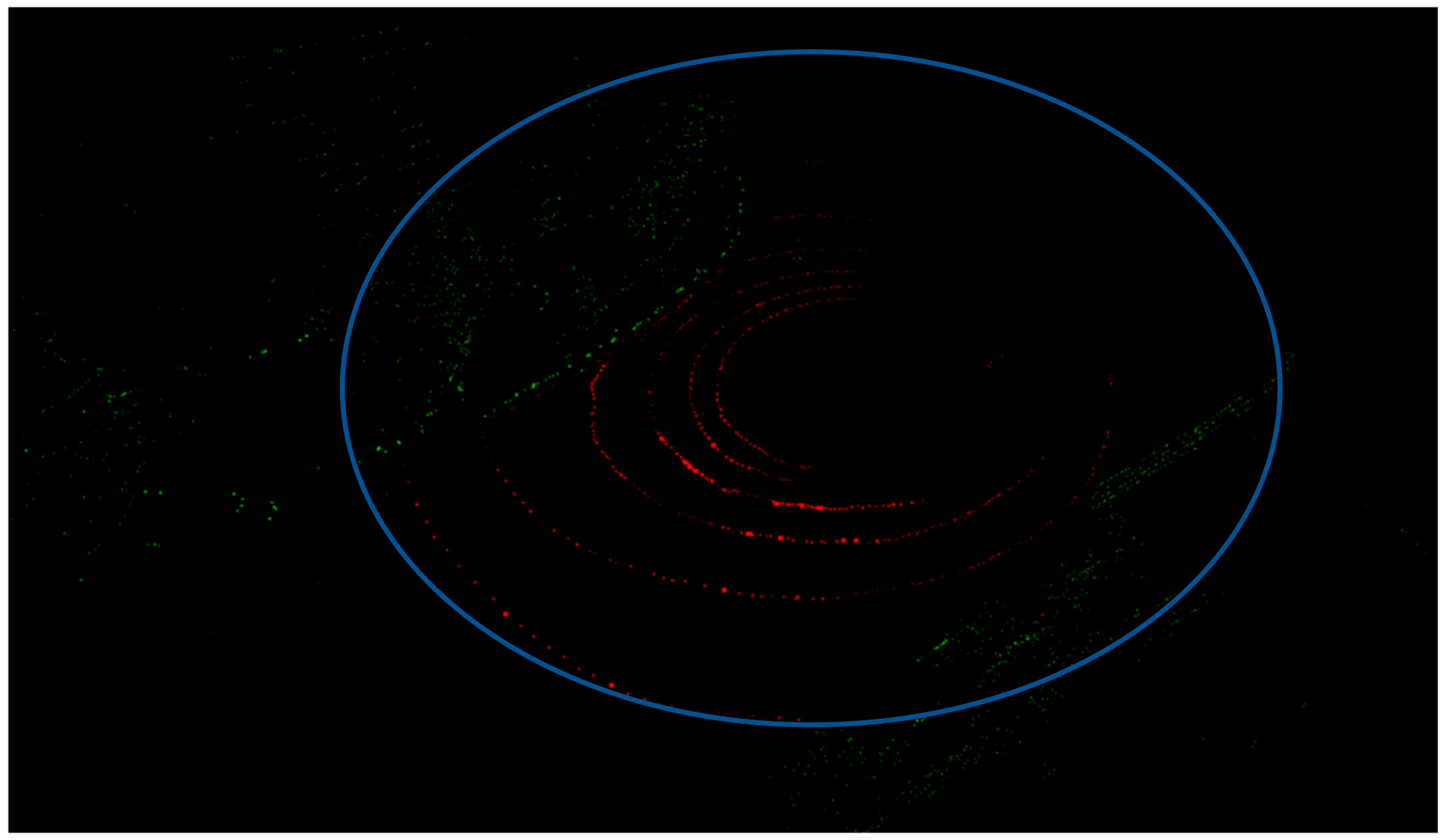
The first derivative of range image was traversed from upper left to lower right; the coordinates of the pixel in image whose first derivative was less than the negative value
were recorded. Next, the second derivative of range image was traversed from this pixel in the row to find the point cloud segment whose second derivative was continuously positive and whose length was greater than or equal to
so as to extract an arc-shaped convex hull (shown in
Figure 2) in the point cloud of dynamic objects (generally including pedestrians and vehicles).
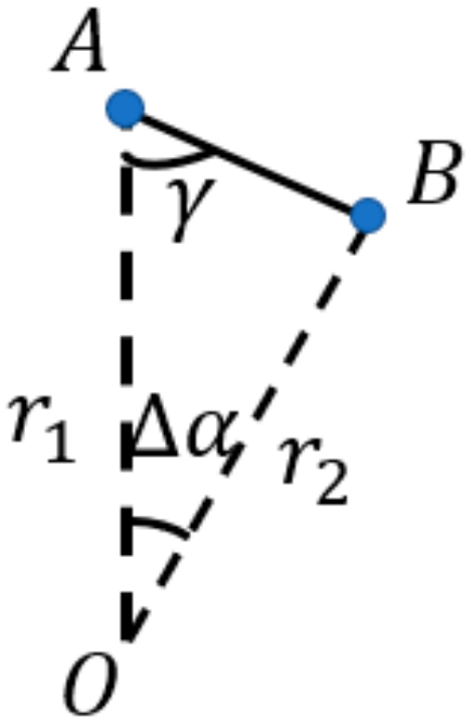
Depth difference between the two ends of the point cloud convex hull was calculated to judge whether this difference was less than or equal to
. The angle γ was calculated between the two end points and the outer point of the adjacent segment, as shown in
Figure 3.
This angle could more stably represent the degree of depth variation of adjacent laser spots, and the angle of the segmented point cloud should have been less than or equal to the threshold value
. The calculation method is as in Equation (7).
The point cloud segment that satisfied the above conditions was taken as segment
, which represents the first segment of scanline
. Considering that the length of the point cloud segment representing a pedestrian’s leg was short and the point cloud of this kind of segment often appeared in the last several lines,
was reduced for segmenting by the line to adapt to this feature. Pseudocode for this process is shown in Algorithm 1.
| Algorithm 1: Segment |
 |
Segments were clustered for dynamic object recognition. The complete point cloud of a dynamic object needed to be composed of multiple segments across the scanlines, so it was necessary to follow the sequence of the scanlines and check
. Segments were clustered according to two criteria. The first criterion was centroid Euclidean distance difference
, which ensured that the distance between the two segments was close enough and isolated segments could not form a dynamic object point cloud. The centroid
was calculated from the points
within the segment.
where
represents number of points within the segment. The second criterion was principal component analysis result of the segment point cloud. Create covariance matrix for all the points contained in the segment, the eigenvector
and the eigenvalue
were calculated, with the eigenvalue and the eigenvector corresponding in turn. For principal component analysis results of the two adjacent segments
and
, Equation (9) needed to be satisfied:
Point cloud segments that met the criteria were clustered to obtain the complete point cloud of dynamic objects. The pseudocode of this algorithm is shown in Algorithm 2.
| Algorithm 2: Cluster |
 |
After clustering was completed, the object point cloud could be identified; those with a number of crossing lines larger than the number of segment points were identified as pedestrians and those with a number of crossing lines smaller than the number of segment points were identified as vehicles. According to the serial number of the point cloud of the dynamic object, range was modified to 0 in the range image to eliminate dynamic point clouds.
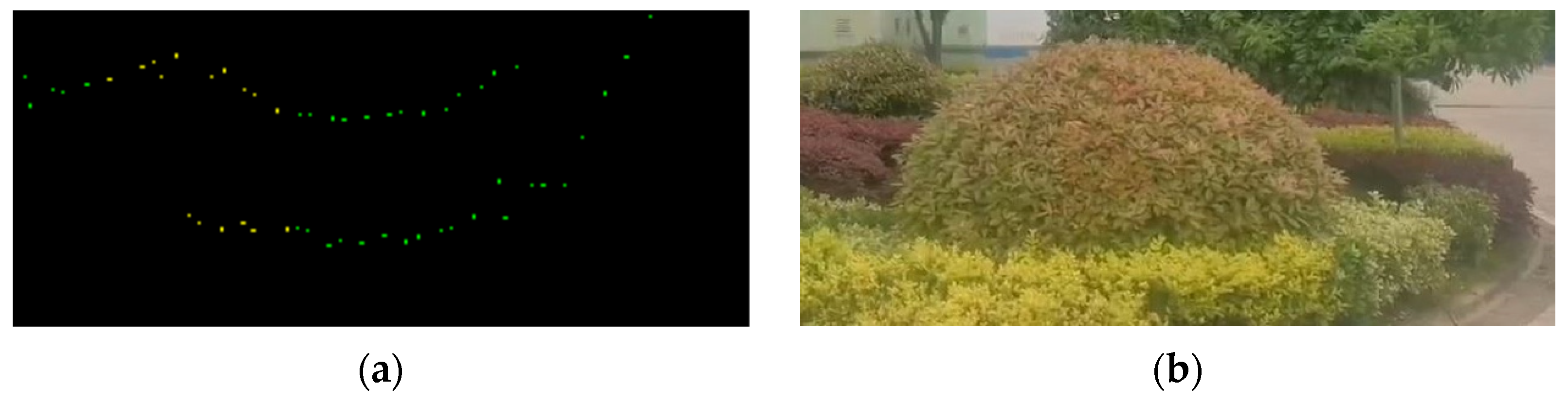
After the dynamic point cloud was eliminated, there was a vacancy in the corresponding position. These missing points were repaired to improve feature point extraction and mapping. First, the second derivative
,
and the first derivative
,
were taken; the first derivative of the endpoint of the vacant segment
,
was calculated. Then, according to the first derivative and the range of the outer endpoints on both sides
,
, the range of the inner endpoints
,
of the vacant segment was calculated. Next, the first derivative and range with the same second derivative toward the inner vacant segment were calculated according to the sequence. The repair of the vacant segment started from both sides and closed in the middle to complete the repair.
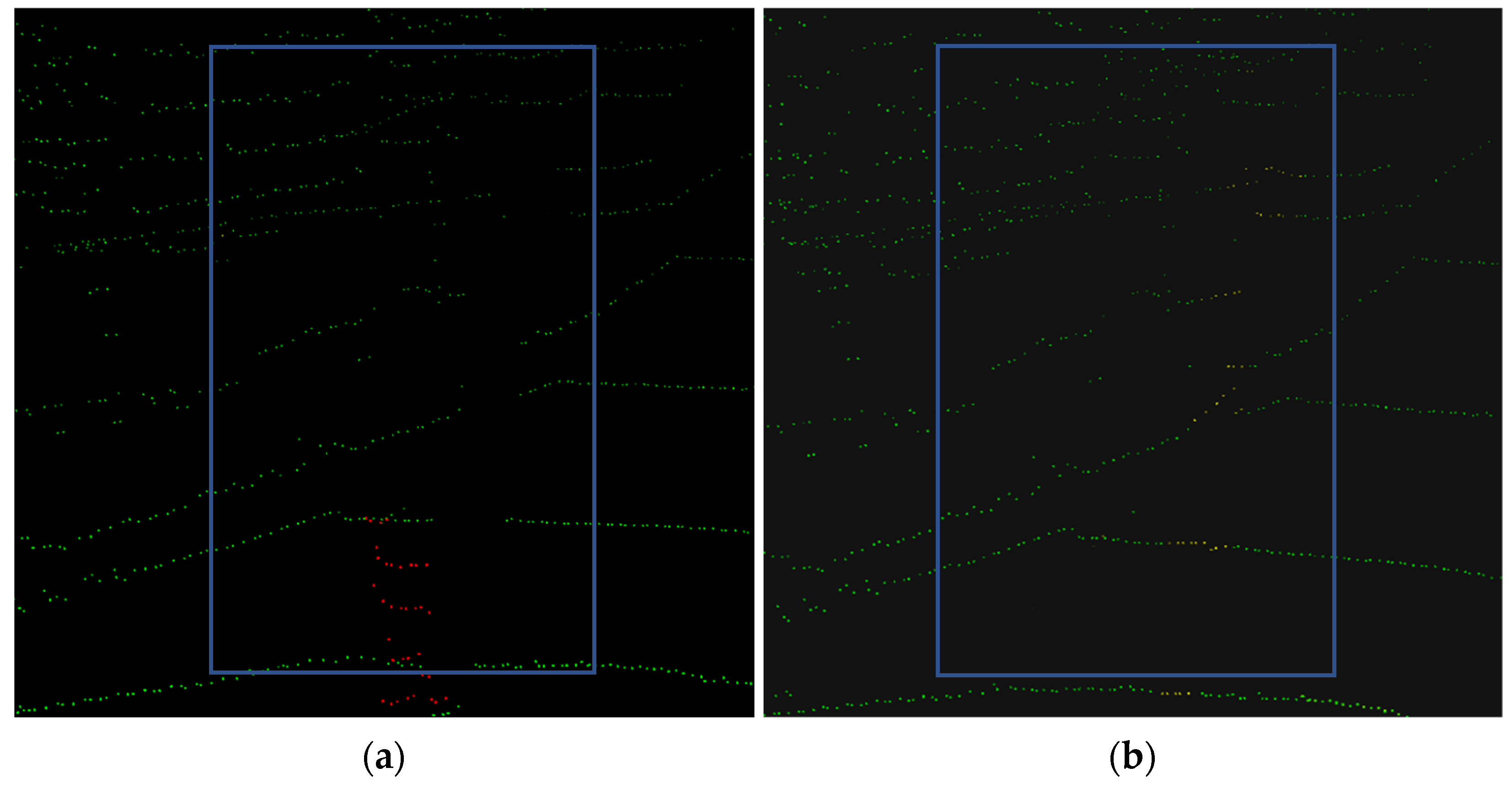
Figure 4 shows the process result of the pedestrian point cloud, in which red points represent the pedestrian point cloud and yellow points are the point cloud of the repaired part.
2.4. Odometry and Mapping
The odometry and mapping process mainly included three parts: feature extraction, odometry and mapping. The LOAM algorithm extracted feature points by calculating curvature and divided the feature points into two types: planar points and edge points. It then matched feature points according to classification. On this basis, we applied ground information for feature extraction. First, the feature extraction strategy was selected according to whether it belonged to the ground. For non-ground areas, in order to ensure uniform distribution of feature points, each scanline was divided into multiple parts according to number of points. The curvature of points in each part was compared with the threshold; those larger than the threshold of edge points were selected as edge points, and those smaller than the threshold of planar points were selected as planar points. The number of edge points and planar points that could be extracted from each part could not exceed the threshold. For the ground area, the planar points were still extracted uniformly, but considering that the ground was relatively flat, extraction density decreased. Because the edge points of the ground were mostly rough ground, the extraction did not consider uniform distribution and only selected several edge points with the largest curvature. In this way, four types of point were extracted: ground edge points, ground planar points, non-ground edge points and non-ground planar points. In odometry and mapping, feature points of each classification were only matched with points of the same classification.
4. Conclusions and Future Work
Aiming at the problems of low positioning accuracy and poor mapping effect of lidar SLAM in dynamic scenes, the authors of this paper carried out a series of research on laser point cloud ground recognition, dynamic object recognition and elimination, localization and mapping, then established a laser point cloud suitable for dynamic scenes. Lidar SLAM algorithm improved the performance of SLAM algorithm in practical applications.
In this paper, a light and fast lidar SLAM algorithm is proposed. Compared with classical LOAM, our algorithm reduced relative position error and relative attitude error obviously (51.6% and 12.5% in the average of straight and bent roads, respectively) within the same running time in a dynamic scene. The algorithm uses a lightweight and embedded object recognition method in the front end to efficiently process the original point cloud so that the processed point cloud features are obvious, which ensures positioning accuracy and facilitates subsequent processing of mapping. A dynamic object recognition algorithm is proposed based on the point cloud harness: using the derivative to represent the point cloud feature. The second derivative should be explicitly used to grow the repaired point cloud from both sides. According to the processing results of the dynamic point cloud, it can be concluded that the algorithm can effectively identify the dynamic point cloud and restore background points occluded by dynamic objects according to the surrounding environment. A processing method of extracting feature points for ground and non-ground classification is proposed. Not only are feature points extracted separately according to categories, but methods for selecting feature points for ground and non-ground categories are different. The proposed algorithm should make feature point extraction more accurate and feature point matching more efficient.
This paper has the following room for improvement: First, the recognition scheme for dynamic objects still needs to be improved. Optimizing the recognition of dynamic objects that are not representative but still appear at different distances and resolutions remains a challenge. It is possible to consider the fusion of millimeter-wave radar to assist in dynamic object recognition and tracking as well as conduct experiments in more dynamic scenarios. Second, the structure of the current algorithm is simple enough to fully meet real-time requirements. The parameters of the process algorithm can be modified, the number of iterations can be increased and the algorithm accuracy can be improved. Other optimization methods can also be introduced in the back end to further improve the accuracy of the algorithm.


