Joint Optimization Strategy of Condition-Based Maintenance and Spare Parts Ordering for Nonlinear Degraded Equipment under Imperfect Maintenance

Abstract

When existing methods consider the impact of the imperfect maintenance activities on random degraded equipment, they usually assume that the degraded equipment is linear, and set the number of imperfect maintenance activities in advance. However, in engineering practice, most of the degraded equipment is nonlinear, and the number of imperfect maintenance activities has an impact on the development of maintenance strategies. Therefore, this paper proposes a new joint maintenance strategy considering the uncertainty of the number of imperfect maintenance activities for nonlinear degraded equipment. First, nonlinear degradation data are linearized based on Box-Cox transformation (BCT), and the degradation model under the influence of imperfect activities is constructed by the random coefficient regression model. Accordingly, the remaining useful life (RUL) probability distribution can be derived. Secondly, the number of maintenances is calculated by imperfect maintenance level and success probability. Then, the detection cycle, preventive maintenance threshold and maintenance times are taken as decision variables. The optimization objective is to minimize the expected average cost. However, this is restricted by availability and probability of success for imperfect maintenance activities. A multi-objective joint optimization model of condition-based maintenance and spare parts ordering is constructed. Finally, the analysis results based on numerical examples verify the feasibility of the proposed joint optimization strategy.

1. Introduction

With the increasingly integrated, intelligent, complex, and precise development of engineering equipment, the cost of equipment testing, replacement and other related maintenance activities has also increased. Therefore, the reliability and economy of equipment operation and maintenance activities have become research interests for a variety of scholars and engineers [1,2]. As a comprehensive technology in the field of equipment reliability, prediction and health management (PHM) provide technical support for the safe and stable operation of equipment. The key point is to predict the remaining life of equipment through degradation monitoring data, and then formulate reasonable maintenance strategies. At the same time, as an important part of PHM, condition-based maintenance (CBM) can improve the safety and reliability of equipment to a certain extent and reduce the occurrence of failure events when considering the actual degradation state of equipment. In practice, the spare parts are naturally stored before the failure for the stochastic degraded equipment, and are adopted to replace the damaged component once the uninterrupted operation of equipment begins. Thus, timely ordering of spare parts can avoid inventory backlogs and reduce cost losses. Based on the RUL prediction information for the degraded equipment, balancing the optimal relationship between CBM and spare parts ordering can effectively improve the reliability of equipment and reduce the operation cost of equipment, so it has important research value and practical significance [3,4,5,6].

In CBM, maintenance activities can be divided into perfect maintenance, imperfect maintenance and minor repair according to the degree of equipment maintenance [7]. Imperfect maintenance refers to the restoration of degraded equipment to a state between new and pre-maintenance by means of maintenance. In contrast, perfect maintenance aims to maintain degraded equipment in a new state. Minor repair aims to maintain the degraded equipment to the state before failure. Compared with perfect maintenance and minor repair, common maintenance activities are generally listed as imperfect maintenance in engineering practice. In the existing research on degradation equipment under imperfect maintenance, Pei et al. [8] constructed the degradation model under imperfect maintenance based on the linear Wiener process, and established the maintenance decision model based on the RUL prediction information and the renewal reward theory. Deep et al. [9] considered the impact of imperfect maintenance activities and modeled the maintenance activities of multiple subsystems. Xu et al. [10] solved the CBM problem based on the Markov process, and considered the influence of imperfect maintenance activities on the optimal decision. Wang et al. [11] considered the degradation model with time-varying covariates and imperfect maintenance activities. Further, Sofiene et al. [12] researched an imperfect maintenance strategy to minimize the maintenance cost by finding the optimal preventive maintenance time and detection cycle for multi-period stochastic fault equipment.

The abovementioned research only concentrated on the decision model for the degradation data of linear equipment. Moreover, the optimization goal for these studies was single, ignoring the joint optimization strategy of nonlinear degraded equipment. The existing methods of degradation data modeling for nonlinear degraded equipment mainly focus on the selection of a transformation method to transform nonlinear degradation data into approximate linear degradation data, and then establish a linear degradation model. Commonly used transformation methods are time scale transformation [13], logarithmic transformation [14], and the nonlinear function method [15]. For example, Wang et al. [16] proposed an optimal replacement strategy for nonlinear degradation equipment based on the nonlinear Wiener process considering the random failure threshold. Wu et al. [17] used exponential distribution to describe nonlinear degradation equipment, and used logarithmic variation to linearize it. By determining the optimal detection interval and degradation degree after imperfect maintenance, a maintenance cost minimization model was established. Zhou et al. [18] constructed a generalized nonlinear Wiener degradation model considering the dependency relationship between the degradation rate and degradation volatility. This model has a time-varying mean-variance ratio and derives the closed solution of approximate RUL so as to further determine the method of estimating the initial value of parameters and time scale function. However, owing to the single application target of time scale transformation and logarithmic transformation, the form of transformation function is limited, which limits its application in practice. At the same time, the method of directly using a nonlinear random model is more dependent on the choice of the nonlinear function, and the nonlinear degradation data in engineering practice to choose which nonlinear function itself is also a problem. In addition, existing methods usually take a single decision function as the optimization objective, ignoring the impact of the multi-objective joint strategy on maintenance decisions.

In view of these limitations, this paper proposes a joint optimization strategy of condition-based maintenance and spare parts ordering for nonlinear degraded equipment under imperfect maintenance. First, the nonlinear degradation data are linearized by Box-Cox transformation (BCT). Compared with time scale transformation and logarithmic transformation, the linear and normal characteristics of the degradation data after BCT are better than those of other transformation techniques, and the function form of BCT is more general. Based on this, the degradation model under imperfect maintenance is constructed by combining the random coefficient regression model, and the cumulative distribution function (CDF) is derived. Second, based on the RUL prediction information and considering the number of imperfect maintenance activities, the joint and optimization strategy of condition-based maintenance and spare parts ordering is constructed. Finally, the effectiveness of the proposed method was verified by numerical simulation. Compared with existing research, this paper introduces the following innovations:

(1)

Compared with the linear degradation modeling method or nonlinear function method used in [8,16], the nonlinear degradation modeling based on BCT in this paper is more general, and the mathematical characteristics of nonlinear degradation data are greatly retained.

(2)

Compared with the maintenance strategy proposed in [10,12,19], the innovation of this paper is to consider the uncertainty of the number of imperfect maintenance activities and compare the influence of the degradation data before and after BCT on the number of imperfect maintenance activities.

(3)

Based on RUL information, a multi-objective joint optimization strategy is established to reasonably maintain and order spare parts, reduce the operation cost of nonlinear degradation equipment and improve availability.

The structure of this paper is as follows: Section 2 describes the issues related to on-the-spot maintenance and spare parts ordering. Section 3 describes the implementation of nonlinear degradation modeling based on BCT and the random coefficient regression model, and further discusses the RUL information obtained. In Section 4, by analyzing the relationship between preventive maintenance, failure maintenance and spare parts ordering, taking the detection cycle, preventive maintenance threshold and maintenance times as decision variables, minimizing expected average cost as the optimization objective, availability and success probability of imperfect maintenance activities as constraints, a multi-objective joint optimization model of condition-based maintenance and spare parts ordering is constructed. Section 5 details the verification of the proposed method through numerical simulation examples. The conclusion is given in Section 6.

2. Problem Description

In engineering practice, existing state monitoring methods can be used to obtain the degradation monitoring data of equipment, so as to analyze the operation state of degraded equipment. When the equipment degradation state exceeds the given preventive maintenance threshold of $w_p$, imperfect maintenance is performed. Considering the mechanical load capacity and economic affordability of the service equipment, the number of maintenance activities $N$ is generally limited to a reasonable range, and each imperfect maintenance activity affects the probability of the next maintenance success. Carrying out frequent maintenance activities increases not only the maintenance cost but also the failure probability of the degraded equipment. After $N$ imperfect maintenance activities for the degraded equipment, when the degradation state exceeds the given failure threshold $w$, it is determined that the degraded equipment fails. In order to avoid degraded equipment shutdown, preventive replacement should be carried out before failure. Figure 1 shows the degradation trajectory of nonlinear degraded equipment under imperfect maintenance, which depicts the time of the second imperfect maintenance activity [20,21].

When the planned failure of the equipment occurs, in order to avoid unnecessary safety problems and economic losses caused by the shutdown of the degraded equipment, spare parts can be ordered in advance and replaced at the time of failure to ensure the stable operation of the equipment. If the equipment fails suddenly, it is necessary to order emergency spare parts immediately and replace the spare parts when the spare parts arrive. However, the loss caused by the shutdown cannot be recovered. Therefore, reasonably optimizing the detection cycle $\Delta t$, preventive maintenance threshold $w_p$ and imperfect maintenance times $N$, and weighing the relationship among them can not only reduce the probability of the sudden failure and maintenance cost of degraded equipment, but also prolong the operation time of equipment and help obtain the optimal maintenance strategy. Based on the above description, the following problems were researched:

(1)

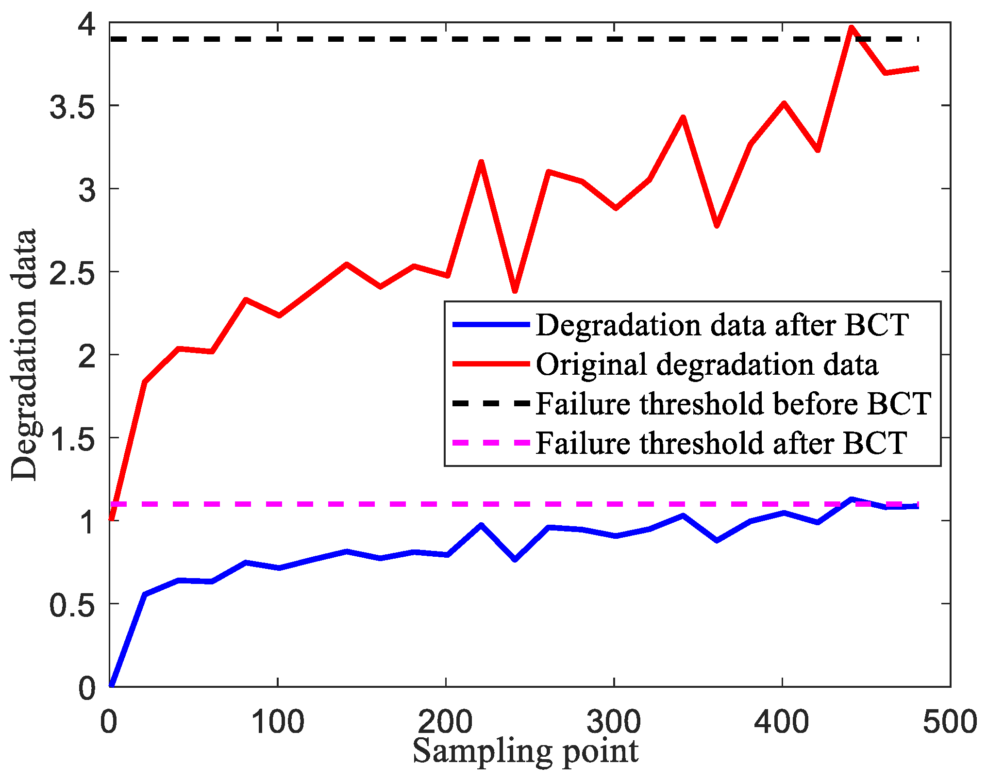
How to find a widely applicable transformation relation to solve the problem of nonlinear degradation data modeling;

(2)

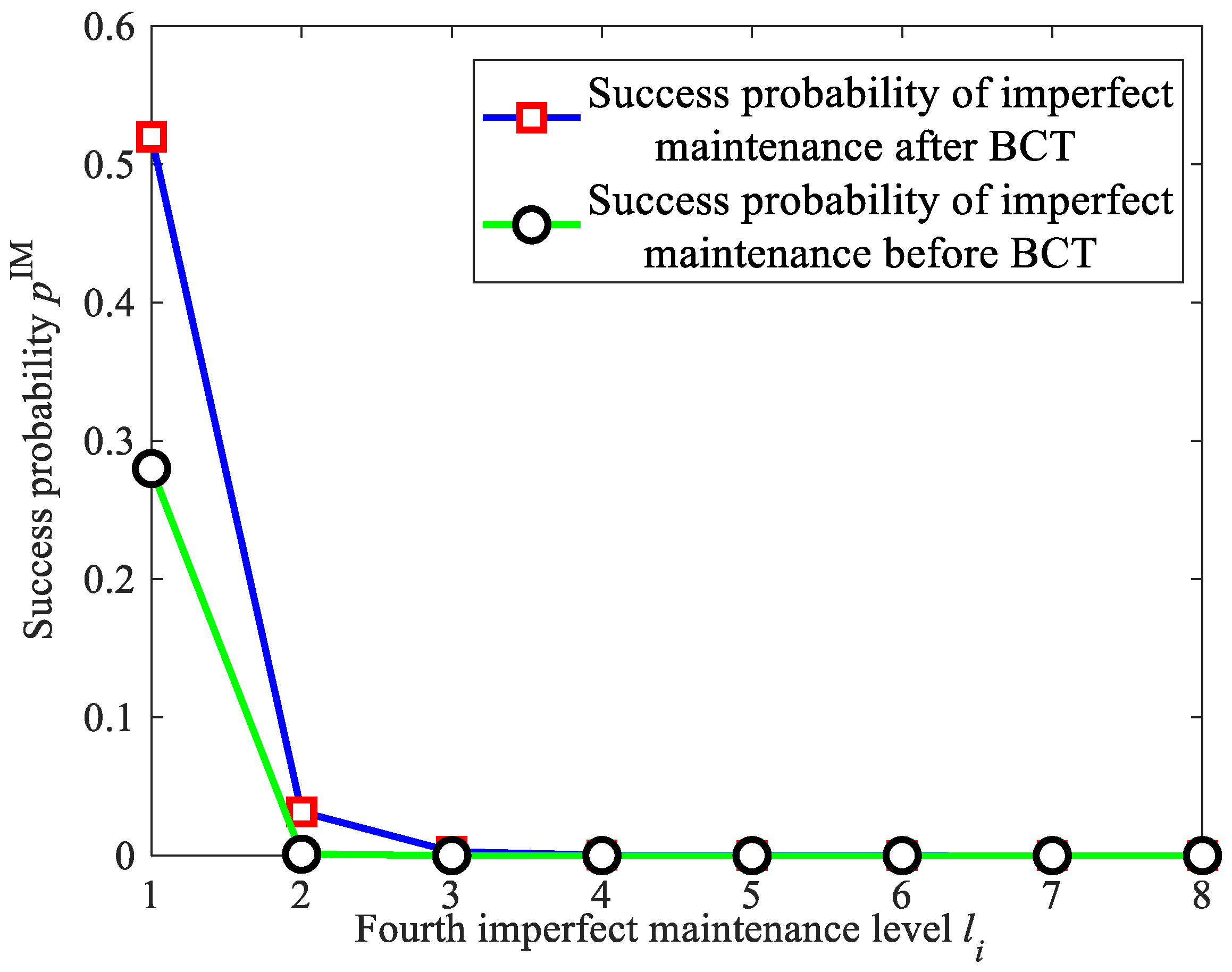
Under the premise that the probability of successful imperfect maintenance activities is known, how to determine and analyze the number of imperfect maintenance activities to achieve the purpose of prolonging the life of degraded equipment;

(3)

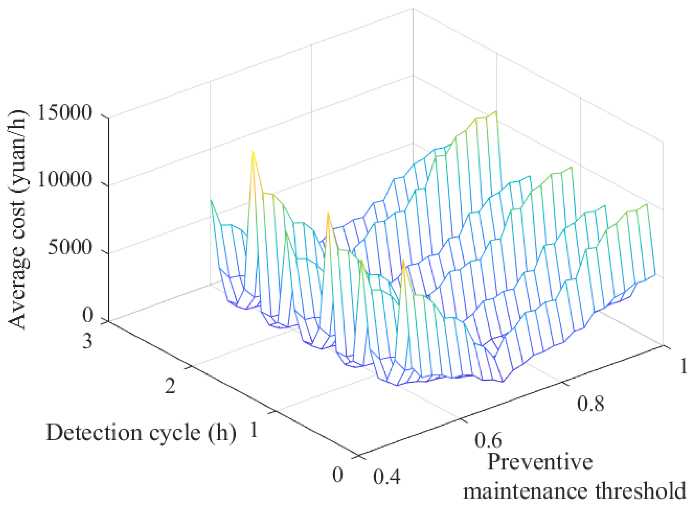
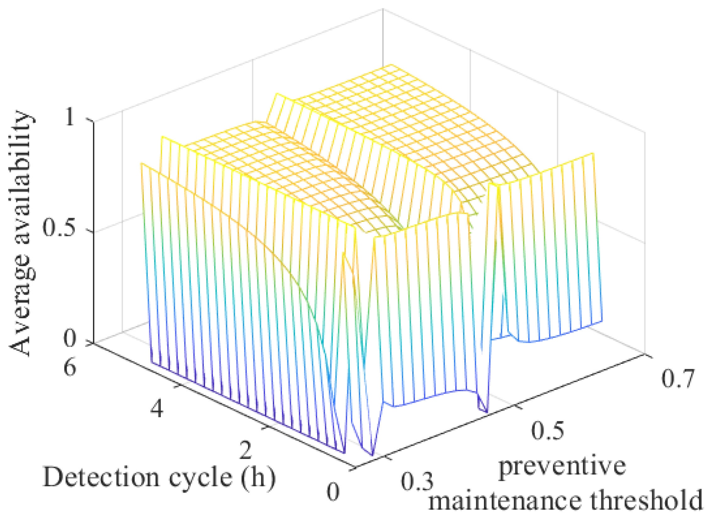
How to reduce the cost of equipment loss per unit time while meeting the availability requirements of degraded equipment.

3. Nonlinear Degradation Modeling and RUL Prediction

For nonlinear degraded equipment, this paper firstly adopts the BCT to linearize the degradation data, and then uses the linear random coefficient regression model to analyze the transformed data. The BCT is a generalized power transformation method proposed by Box and Cox in 1964 [22], which has since been applied in many fields. The optimal BCT can be obtained by calculating and analyzing the transformation parameters to improve the linearity, independence, homogeneity of variance, and normality of the original degradation data. Its general form can be expressed as

$$Z\left(t,\lambda \right)=\{\begin{array}{c}\frac{X{\left(t\right)}^{\lambda }-1}{\lambda },\lambda \ne 0\hfill \\ \log X\left(t\right),\lambda =0\hfill \end{array}$$

(1)

where, $X\left(t\right)$ is the original degradation, $\lambda$ is the transformation parameter, $Z\left(t,\lambda \right)$ is the transformation degradation. The corresponding inverse transformation can be expressed as

$$X(t)=\{\begin{array}{c}{\left(1+\lambda Z\left(t,\lambda \right)\right)}^{\frac{1}{\lambda }},\lambda \ne 0\\ \exp Z\left(t,\lambda \right),\lambda =0\end{array}$$

(2)

For the transformed degradation variable $Z\left(t,\lambda \right)$, considering the nonlinear data linearization ability of the BCT, this paper utilizes the linear random coefficient regression model to describe the equipment degradation process under imperfect maintenance. After the $k$th preventive maintenance activity, the degradation of equipment in the $\left(k+1\right)$th phase can be formulated as

$$Z_k\left(t,\lambda \right)={\delta }_k+{\phi }_k+{\theta }_k\left(t-{\widehat{t}}_k\right)+\epsilon$$

(3)

where, ${\delta }_k$ represents the residual degradation level of nonlinear degraded equipment after the $k$th maintenance activity, describing the influence of maintenance activities on the degradation process of nonlinear degraded equipment. Specially, we have ${\delta }_0=0$. The figure ${\phi }_k$ represents the fixed parameter. Without loss of generality, let ${\phi }_k=0$. The figure ${\widehat{t}}_k$ represents the $k$th maintenance activity time. The symbol ${\theta }_k$ represents the stochastic effect coefficient after the $k$th maintenance activity to characterize the individual differences between devices, ${\theta }_0$ represents the random effect coefficient before maintenance, and ${\theta }_k=\left(k+1\right){\theta }_0$, ${\theta }_0\sim N\left({\mu }_0,{\sigma }_0^2\right)$, ${\theta }_k~N\left({\mu }_k,{\sigma }_k^2\right)$. Next, $\epsilon$ is the noise term, indicating the random error, and $\epsilon \sim N\left(0,{\sigma }^2\right)$. Parameters are independent of each other. In order to simplify the analysis process of the model, we write the degradation of the equipment after BCT at ${\widehat{t}}_k$ time as $Z_k^{\left(\lambda \right)}$, and the model can be written as

$$Z_k^{\left(\lambda \right)}={\delta }_k+{\theta }_k\left(t-{\widehat{t}}_k\right)+\epsilon$$

(4)

In order to facilitate subsequent calculation and research, it is generally assumed that the residual degradation level ${\delta }_k$ in Equation (4) follows the Gaussian distribution [23], but such an assumption cannot solve the problem that the residual degradation amount is negative. Based on the above considerations, the references [24,25] introduced Beta distribution to solve this problem. The value of residual degradation quantity ${\delta }_k$ can be constrained in the range of $\left(0,1\right)$. Therefore, this paper assumes that the probability density function (PDF) of residual degradation is expressed as

$$f\left({\delta }_k\right)=\{\begin{array}{cc}\frac{\mathsf{\Gamma }\left({\alpha }_1^{k-1}+{\alpha }_2\right)}{\mathsf{\Gamma }\left({\alpha }_1^{k-1}\right)\mathsf{\Gamma }\left({\alpha }_2\right)}{\delta }_k^{{\alpha }_1^{k-1}-1}{\left(1-{\delta }_k\right)}^{{\alpha }_2-1}& 1<k\le N+1\hfill \\ 0& k=1\hfill \end{array}$$

(5)

where, ${\alpha }_1$ and ${\alpha }_2$ are hyper-parameters, which can be estimated by the maximum likelihood estimation method.

According to the characteristics of the Beta distribution, the mathematical expectation of residual degradation is obtained as follows

$${\rm E}\left({\delta }_k\right)=\frac{{\alpha }_1^{k-1}}{{\alpha }_1^{k-1}+{\alpha }_2}$$

(6)

It is obvious that with continuous imperfect maintenance activities, the larger the degradation level, the greater the likelihood of the value range conforming to the assumption of the model.

Assuming that the model in this paper follows a Gaussian distribution with parameter $\left({\mu }_{k,z}^{\left(\lambda \right)},{\sigma }_{k,z}^{2\left(\lambda \right)}\right)$, when the residual degradation ${\delta }_k$ after the $k$th preventive maintenance activity is known, we have

$${\mu }_{k,z}^{\left(\lambda \right)}={\mu }_k·\left(t-{\widehat{t}}_k\right)$$

(7)

$${\sigma }_{k,z}^{2\left(\lambda \right)}={\sigma }_k^2·{\left(t-{\widehat{t}}_k\right)}^2+{\sigma }^2$$

(8)

In this paper, it is assumed that the degradation process $Z\left(t,\lambda \right)$ fails when it reaches the given failure threshold $w$, so that the distribution of RUL is transformed into the time distribution of the degradation process reaching the failure threshold. Taking into account the definition of RUL, and the nonnegative feature, the PDF and CDF of the time to reach the preventive maintenance threshold $w_p$ and failure threshold $w$ can be obtained, as

$$f_{k,w_p}\left(t_k,w_p|{\delta }_k\right)=\frac{\varphi \left({\varsigma }_p\left(t_k,w_p|{\delta }_k\right)\right)·{{\varsigma }^{\prime }}_p\left(t_k,w_p|{\delta }_k\right)}{1-\mathrm{\Phi }\left({\varsigma }_p\left(0|{\delta }_k\right)\right)}$$

(9)

$$f_{k,w}\left(t_k,w|{\delta }_k\right)=\frac{\varphi \left({\varsigma }_w\left(t_k,w|{\delta }_k\right)\right)·{{\varsigma }^{\prime }}_w\left(t_k,w|{\delta }_k\right)}{1-\mathrm{\Phi }\left({\varsigma }_w\left(0|{\delta }_k\right)\right)}$$

(10)

$$F_{k,w_p}\left(t_k,w_p|{\delta }_k\right)=\frac{\mathrm{\Phi }\left({\varsigma }_p\left(t_k,w_p|{\delta }_k\right)\right)-\mathrm{\Phi }\left({\varsigma }_p\left(0|{\delta }_k\right)\right)}{1-\mathrm{\Phi }\left({\varsigma }_p\left(0|{\delta }_k\right)\right)}$$

(11)

$$F_{k,w}\left(t_k,w|{\delta }_k\right)=\frac{\mathrm{\Phi }\left({\varsigma }_w\left(t_k,w|{\delta }_k\right)\right)-\mathrm{\Phi }\left({\varsigma }_w\left(0|{\delta }_k\right)\right)}{1-\mathrm{\Phi }\left({\varsigma }_w\left(0|{\delta }_k\right)\right)}$$

(12)

where, $\varphi (·)$ denotes the PDF of standard normal random variables and $\mathrm{\Phi }(·)$ is the CDF of the standard normal random variables, ${\varsigma }_p\left(t_k,w_p|{\delta }_k\right)=\frac{{\mu }_{k,z}^{\left(\lambda \right)}-w_p-{\delta }_k}{\sqrt{{\sigma }_{k,z}^{2\left(\lambda \right)}}}$, ${\varsigma }_w\left(t_k,w|{\delta }_k\right)=\frac{{\mu }_{k,z}^{\left(\lambda \right)}-w-{\delta }_k}{\sqrt{{\sigma }_{k,z}^{2\left(\lambda \right)}}}$.

4. Joint Optimization Model of Conditional Maintenance and Spare Parts Ordering

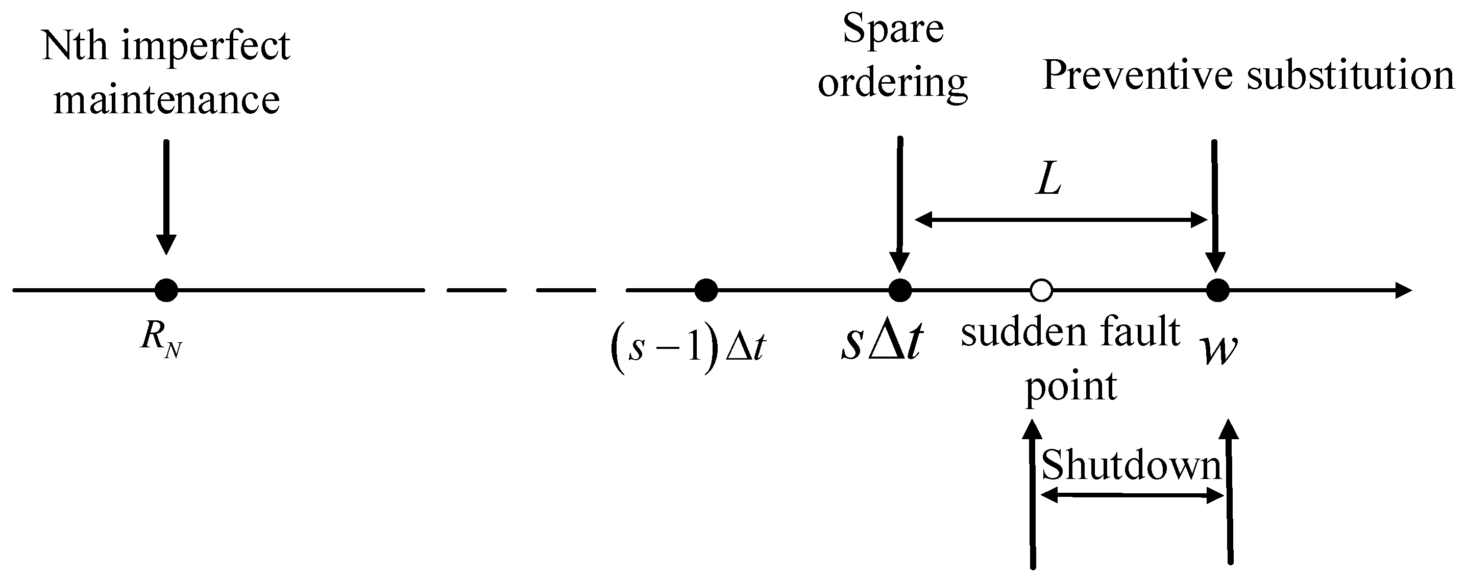
After each spare part replacement, the equipment enters a new life cycle, namely a new state. The need for spare parts ordering is divided into four cases:

(1)

After $N$ imperfect maintenance activities, the equipment fails between the spare parts ordering and the expected failure time, and the standby spare parts need to be replaced.

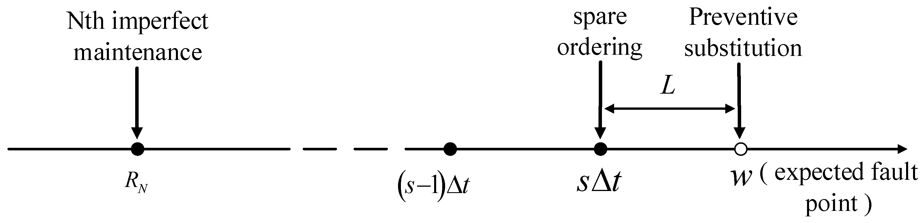
(2)

After $N$ imperfect maintenance activities, the equipment normally fails at the expected failure time, which requires the replacement of spare parts without shutdown;

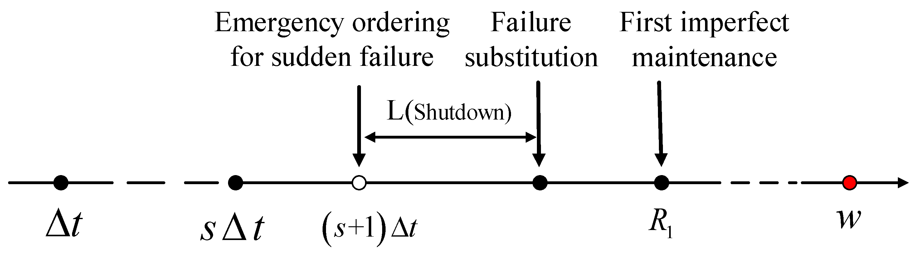
(3)

After $N$ imperfect maintenance activities, the equipment fails before the expected spare parts ordering time, which requires emergency spare parts ordering and replacement of downtime spare parts;

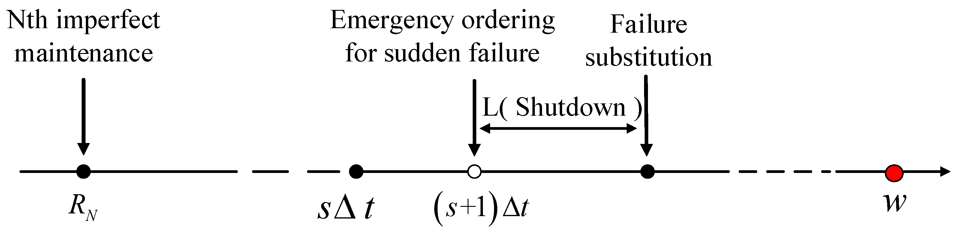
(4)

Without imperfect maintenance of equipment, sudden failure occurs. At this time, emergency spare parts ordering and shutdown spare parts replacement are needed.

Based on the above analysis, this paper assumes the following:

(1)

During the life cycle, the cost of each test is $C_d$, the cost of preventive maintenance is $C_{pm}$, the cost of preventive replacement is $C_{pr}$, the cost of invalid replacement is $C_l$, the cost of expected spare parts is $C_{ps}$, the cost of emergency ordering spare parts for sudden failure is $C_u$, the downtime cost caused by the inability to replace spare parts is $C_t$, and the spare parts order time is $L$;

(2)

The detection time and spare parts replacement time are ignored;

(3)

The downtime cost per unit time is certain;

(4)

Considering the cost relationship in engineering practice, let $C_l>C_{pr}>C_{pm}>C_d$, $C_u>C_{ps}$.

4.1. Number of Imperfect Maintenance Activities

This paper assumes that there are $M+1$ different states in the degradation process for nonlinear equipment, that is $\left(0,1,\cdots ,M\right)$, where $0$ means failure, $M$ means perfect as new, and the intermediate state is between $0$ and $M$. Degradation monitoring data for equipment status are shown in Equation (13).

$$\underset{M}{\underbrace{z_1,z_2,\cdots ,z_i}},\underset{M-1}{\underbrace{z_{i+1},\cdots ,z_{2i}}},\cdots ,\underset{1}{\underbrace{z_{\left(M-1\right)i+1},\cdots ,z_{Mi}}},\underset{0}{\underbrace{z_{Mi+1},\cdots ,z_{\left(M+1\right)i}}}$$

(13)

As shown in Figure 2, maintenance activities are equivalent to rectifying the degradation trend of the state of the equipment, and perfect maintenance is more complete than imperfect maintenance activities. The preventive maintenance threshold $w_p$ corresponds to a certain intermediate state (e.g., the state $1$ in Figure 2), and the failure threshold $w$ corresponds to the state $0$. When the equipment state degenerates to state $1$, imperfect maintenance is implemented, but the maintenance result is considered to be random because the equipment may be in any intermediate state after maintenance. At the same time, with the accumulation of imperfect maintenance activities, the probability that the device can be maintained to a near perfect state is gradually reduced. For example, the degradation state of a piece of nonlinear equipment is $\left(0,1,2,3,4\right)$. It is generally believed that the probability of successfully maintaining the degraded equipment from state $0$ to state $4$ is the lowest, and only the equipment can be replaced. At the same time, the probability of successfully maintaining the degraded equipment from state 1 to state 2 is higher than from state 1 to state 3.

Let $l_i\left(0<i<M\right)$ denote the imperfect maintenance level, for example, $l_2$ denotes the maintenance from state $1$ to state $3$. The figure $N$ indicates the number of imperfect maintenance activities. Considering the influence of the number of previous imperfect maintenance activities and the imperfect maintenance level, the probability of the next successful imperfect maintenance activity can be updated as

$$p_{i+1}^{IM}\left(N,l_i\right)=p_i^{IM}\left(N,l_i\right)·\exp \left(-N·\frac{l_i}{M}\right)$$

(14)

In the formula, $p_1^{IM}$ represents the probability of success for the first imperfect maintenance activity, which is generally determined by expert experience and historical data. The optimal number of imperfect maintenance activities can be obtained according to the minimum threshold $p_m^{IM}$ and the imperfect maintenance level for successful imperfect maintenance activities.

4.2. Preventive Replacement and Spare Parts Ordering

After preventive maintenance, preventive replacement is needed before the degradation state of the equipment exceeds the failure threshold. It is assumed that the preventive replacement time is $s\Delta t\left(s>N\right)$, and the $k$th $\left(0<k\le N\right)$ preventive maintenance time is $j_k\Delta t$. For the preventive maintenance probability $p_p\left(j_k\right)$ at the $j_k\Delta t$ time, lemma 1 [8] is given to calculate the corresponding expressions.

Lemma 1. 

stochastic degraded equipment under imperfect maintenance and preventive maintenance probability$p_p\left(j_k\right)$at $j_k\Delta t$is

$$\begin{array}{ll}{p}_p\left(j_k\right)=& {\displaystyle {\int }_0^{w_p}\{\left(1-F_{k-1,w_p}\left(\left(j_k-j_{k-1}-1\right)\Delta t|{\delta }_{k-1}\right)\right)·{\displaystyle {\int }_{{\delta }_{k-1}}^{w_p}{f}_{k-1,\varphi }\left(z;\left(j_k-j_{k-1}-1\right)\Delta t\right)·}}\hfill \\ & \left(F_{k-1,w_p-z}\left(\Delta t,z|{\delta }_{k-1}\right)-F_{k-1,w-z}\left(\Delta t,z|{\delta }_{k-1}\right)\right)dz\}f\left({\delta }_{k-1}\right)d{\delta }_{k-1}\hfill \end{array}$$

(15)

where,

$f_{k,\varphi }\left(z;t\right)=\frac{1}{\sqrt{2\pi {\sigma }^2}}\exp \left[-\frac{{\left(z-{\delta }_k-{\theta }_{k}t\right)}^2}{2{\sigma }^2}\right]$, $f_{k,w_p-z}\left(\kappa ,z|{\delta }_k\right)=\frac{\varphi \left({\varsigma }_{k,p}\left(\kappa ,w_p\right)\right)·{{\varsigma }^{\prime }}_{k,p}\left(\kappa ,w_p\right)}{1-\mathrm{\Phi }\left({\varsigma }_{k,p}\left(0\right)\right)}$,

$f_{k,w-z}\left(\kappa ,z|{\delta }_k\right)=\frac{\varphi \left({\varsigma }_{k,w}\left(\kappa ,w\right)\right)·{{\varsigma }^{\prime }}_{k,w}\left(\kappa ,w\right)}{1-\mathrm{\Phi }\left({\varsigma }_{k,w}\left(0\right)\right)}$, $F_{k,w_p-z}\left(\kappa ,z|{\delta }_k\right)=\frac{\mathrm{\Phi }\left({\varsigma }_{k,p}\left(\kappa ,w_p\right)\right)-\mathrm{\Phi }\left({\varsigma }_{k,p}\left(0\right)\right)}{1-\mathrm{\Phi }\left({\varsigma }_{k,p}\left(0\right)\right)}$,

$F_{k,w-z}\left(\kappa ,z|{\delta }_k\right)=\frac{\mathrm{\Phi }\left({\varsigma }_{k,w}\left(\kappa ,w\right)\right)-\mathrm{\Phi }\left({\varsigma }_{k,w}\left(0\right)\right)}{1-\mathrm{\Phi }\left({\varsigma }_{k,w}\left(0\right)\right)}$, ${\varsigma }_{k,p}\left(\kappa ,w_p\right)=\frac{{\mu }_k·\kappa -w_p-z}{\sqrt{{\sigma }_k^2·{\kappa }^2+{\sigma }^2}}$,

${\varsigma }_{k,w}\left(\kappa ,w\right)=\frac{{\mu }_k·\kappa -w-z}{\sqrt{{\sigma }_k^2·{\kappa }^2+{\sigma }^2}}$.

The proof process is given in [8], so there is no discussion of it given here.

Based on Lemma 1, the probability of the preventive replacement of degraded equipment at $s\Delta t$ is $p_p\left(s,N\right)$, which can be denoted as

$$\begin{array}{ll}{p}_p\left(s,N\right)=& {\displaystyle \sum _{j_1=1}^{s-N+1}{\displaystyle \sum _{j_2=j_1+1}^{s-N+2}\cdots }}{\displaystyle \sum _{j_N=j_{N-1}+1}^s\{{\displaystyle {\prod }_{s=1}^N{p}_p\left(j_k\right)}}·p_p[Z\left(s\Delta t\right)<w_p\cap w_p\le Z\left(\left(s+1\right)\Delta t<w\right)]\hfill \\ \hfill =& {\displaystyle \sum _{j_1=1}^{s-N+1}{\displaystyle \sum _{j_2=j_1+1}^{s-N+2}\cdots }}{\displaystyle \sum _{j_N=j_{N-1}+1}^s\{}{\displaystyle {\prod }_{k=1}^N{p}_p\left(j_k\right)}·{\displaystyle {\int }_0^{w_p}\{}\left(1-F_{N,w_p}\left(\left(s-j_N\right)\Delta t|{\delta }_N\right)\right)·\hfill \\ & {\displaystyle {\int }_{{\delta }_N}^{w_p}{f}_{N,\varphi }\left(z;\left(s-j_N\right)\Delta t\right)}·\left(F_{N,w_p-z}\left(\Delta t,z|{\delta }_N\right)-F_{N,w-z}\left(\Delta t,z|{\delta }_N\right)\right)dz\}·f\left({\delta }_N\right)d{\delta }_N\}\hfill \end{array}$$

(16)

The probability of the preventive replacement of degraded equipment after preventive maintenance is

$$p_p\left(\Delta t,N,w_p\right)={\displaystyle {\sum }_{s=N}^{\infty }{p}_p\left(s,N\right)}$$

(17)

Next, combined with preventive replacement and spare parts ordering, two situations are studied.

Case 1: 

After$N$imperfect maintenance activities, the equipment fails after the spare parts ordering, and the failure time is less than$w$. The specific process is shown in Figure 3. The figure $L$indicates the time from spare parts ordering to spare parts arrival.

The equipment downtime is

$$T_1=L-{\displaystyle {\int }_{s\Delta t}^{s\Delta t+L}{f}_{k,w_p}\left(t_k,w_p\right)}d{t}_k$$

(18)

The probability of event occurrence is

$$\begin{array}{ll}\hfill p_1& =p\left\{T\le w_p|T>R_N+k\Delta t\right\}=\frac{p\left(R_N+s\Delta t<T\le w_p\right)}{p\left(T>R_N+s\Delta t\right)}\hfill \\ & =\frac{f_{k,w_p}\left(R_N+s\Delta t\right)-f_{k,w_p}\left(w_p\right)}{f_{k,w_p}\left(R_N+k\Delta t\right)}=1-\frac{f_{k,w_p}\left(w_p\right)}{f_{k,w_p}\left(R_N+s\Delta t\right)}\hfill \end{array}$$

(19)

Case 2: 

After$N$imperfect maintenance activities, the equipment fails at the expected failure point, and the failure time is equal to$w$. At this point, the degraded equipment does not produce shutdown events, as shown in Figure 4.

The equipment downtime is

$$T_2=0$$

(20)

The probability of event occurrence is

$$p_2=p_p-p_1$$

(21)

4.3. Failure Substitution and Spare Parts Ordering

The probability of preventive replacement has been found in Section 4.2. According to the concept of opposite events, the probability of failure replacement is

$$p_l\left(\Delta t,n,w_p\right)=1-p_p\left(\Delta t,N,w_p\right)=1-{\displaystyle {\sum }_{s=N}^{\infty }{p}_p\left(s,N\right)}$$

(22)

In engineering practice, the degraded equipment can fail at any time, so it may be assumed that $\left(k+1\right)\Delta t$ is the failure time. According to whether the degraded equipment has experienced maintenance activities or not, the failure replacement is also divided into two cases: (1) Without maintenance activities before the failure of degraded equipment; (2) the degraded equipment experiences $n\left(0<n\le N\right)$ preventive maintenance activities before failure. When failure replacement is combined with spare parts ordering, the decision process is as follows.

Case 3: 

Without maintenance activities before the sudden failure, the emergency spare parts ordering is executed at the time of failure, and the spare parts are replaced immediately when the spare parts arrive. The specific process is shown in Figure 5.

The equipment downtime is

$$T_3=L$$

(23)

The probability of event occurrence is

$$\begin{array}{ll}\hfill p_3& =p\left(Z\left(s\Delta t\right)<w_p\cap Z\left(\left(s+1\right)\Delta t\right)>w\right)\hfill \\ & =p\left(Z\left(s\Delta t\right)<w_p\cap Z\left(\left(s+1\right)\Delta t\right)-Z\left(s\Delta t\right)>w-Z\left(s\Delta t\right)\right)\hfill \\ & ={\displaystyle {\int }_{s\Delta t}^{\infty }{f}_{0,w_p}}\left(t_0\right)d{t}_0·{\displaystyle {\int }_0^{\Delta t}{\displaystyle {\int }_0^{w_p}{f}_{0,\varphi }\left(z;s\Delta t\right)·f_{0,w-z}\left(\kappa ,z\right)d\kappa dz}}\hfill \\ & =\left(1-F_{0,w_p}\left(k\Delta t\right)\right)·{\displaystyle {\int }_0^{w_p}{f}_{0,\varphi }\left(z;k\Delta t\right)}·F_{0,w-z}\left(\Delta t,z\right)dz\hfill \end{array}$$

(24)

where,

$f_{0,\varphi }\left(z;t\right)=\frac{1}{\sqrt{2\pi {\sigma }^2}}\exp \left[-\frac{\left(z-{\theta }_{0}t\right)}{2{\sigma }^2}\right]$, $f_{0,w-z}\left(\kappa ,z\right)=\frac{\varphi \left({\varsigma }_{0,w}\left(\kappa ,w\right)\right)·{{\varsigma }^{\prime }}_{0,w}\left(\kappa ,w\right)}{1-\mathrm{\Phi }\left({\varsigma }_{0,w}\left(0\right)\right)}$,

$F_{0,w-z}\left(\kappa ,z\right)=\frac{\mathrm{\Phi }\left({\varsigma }_{0,w}\left(\kappa ,w\right)\right)-\mathrm{\Phi }\left({\varsigma }_{0,w}\left(0\right)\right)}{1-\mathrm{\Phi }\left({\varsigma }_{0,w}\left(0\right)\right)}$, ${\varsigma }_{0,p}\left(\kappa ,w_p\right)=\frac{{\mu }_{0,z}^{\left(\lambda \right)}-w_p-z}{\sqrt{{\sigma }_{0,z}^{2\left(\lambda \right)}}}$, ${\varsigma }_{0,w}\left(\kappa ,w\right)=\frac{{\mu }_{0,z}^{\left(\lambda \right)}-w-z}{\sqrt{{\sigma }_{0,z}^{2\left(\lambda \right)}}}$.

Case 4: 

After$n$preventive maintenance activities before failure, emergency spare parts ordering is performed at the time of failure, and spare parts are replaced immediately when the spare parts arrive. The specific process is shown in Figure 6.

The downtime is

$$T_4=L$$

(25)

The probability of the event occurrence is

$$\begin{array}{ll}\hfill p_4=& {\displaystyle \sum _{j_1=1}^{s-n+1}}{\displaystyle \sum _{j_2=j_1+1}^{s-n+2}\cdots }{\displaystyle \sum _{j_N=j_{n-1}+1}^s\{{\displaystyle {\prod }_{s=1}^n{p}_p\left(j_k\right)·{\displaystyle {\int }_0^{w_p}\{\left(1-F_{n,w_p}\left(\left(s-j_n\right)\Delta t|{\delta }_n\right)\right)}·}}\hfill \\ & {\displaystyle {\int }_{{\delta }_n}^{w_p}{f}_{n,\varphi }\left(z;\left(s-j_n\right)\Delta t\right)}·F_{n,w-x}\left(\Delta t,z|{\delta }_n\right)dz\}·f\left({\delta }_n\right)d{\delta }_n\}\hfill \end{array}$$

(26)

Based on the above analysis, combined with the renewal reward theory, we can further derive the following equations:

$$ET={\displaystyle \sum _{s=n}^{\infty }\left[{\displaystyle \sum _{n=0}^N\left(s+1\right)\Delta t·p_l\left(\Delta t,n,w_p\right)}\right]}+{\displaystyle \sum _{s=N}^{\infty }\left[s\Delta t·p_p\left(\Delta t,N,w_p\right)\right]}$$

(27)

$$\begin{array}{ll}\hfill EC=& p_p\left[E\left(N_m\right)C_{pm}+E\left(N_d\right)C_d+C_{ps}+C_{pr}\right]\hfill \\ & +p_3\left[E\left(N_m\right)C_{pm}+E\left(N_d\right)C_d+C_u+C_l\right]\hfill \\ & +p_4\left[E\left(N_d\right)C_d+C_u+C_l\right]\hfill \end{array}$$

(28)

$$ES={\displaystyle \sum _{k=1}^N\left(T_1{p}_1+T_2{p}_2+T_3{p}_3+T_4{p}_4\right)}$$

(29)

$$E\left(N_m\right)=\frac{ET}{\Delta t}$$

(30)

$$E\left(N_d\right)={\displaystyle \sum _{k=0}^{\infty }{\displaystyle \sum _{n=0}^{N}n{p}_l\left(\Delta t,n,w_p\right)}}+{\displaystyle \sum _{k=0}^{\infty }{\displaystyle \sum _{n=0}^{N}n{p}_p\left(\Delta t,N,w_p\right)}}$$

(31)

The figure $ET$ represents the life cycle of degraded equipment, $EC$ represents the expected cost of the life cycle, $ES$ represents the expectation of downtime, $E\left(N_m\right)$ represents the expectation of preventive maintenance times, and $E\left(N_d\right)$ represents the expectation of detection times.

Therefore, the average cost model of the degraded equipment’s life cycle is

$$E\left(\Delta t,w_p,N\right)=\frac{EC}{ET}$$

(32)

The average availability of degraded equipment is

$$A\left(\Delta t,w_p,N\right)=\frac{ET}{ET+ES}$$

(33)

Combining Equations (14), (32), and (33), based on the given minimum threshold for successful preventive maintenance activities and the derived RUL prediction information, the joint optimization model of maintenance and spare parts ordering is constructed.

$$\{\begin{array}{c}\min \left(E\left(\Delta t,w_p,N\right)\right)\\ s.t. A\left(\Delta t,w_p,N\right)\ge A_p\\ s.t. p_i^{IM}\left(N,l_i\right)\ge p_m^{IM}\end{array}$$

(34)

First, according to the degradation data before and after BCT, combined with Equation (14), the number of imperfect maintenance activities $p_1^{IM}$ is deduced under the premise of a given $N$. Further, $N$ is substituted into Equations (32) and (33), and the decision variables $\Delta t$ and $w_p$ are optimized by MATLAB. The joint optimization of Equation (34) is realized, and the optimal detection period, spare parts ordering threshold and preventive maintenance times are obtained. The average expected cost of degraded equipment is minimized after a reasonable number of preventive maintenance activities and the purpose of life extension of degraded equipment is achieved.

5. Discussion on Experimental Analysis

In order to verify the effectiveness and applicability of the joint optimization model for the maintenance strategy of nonlinear degradation equipment, we used numerical examples to carry out simulation experiments. Based on the model in this paper, the degradation data are simulated. Given the transformation parameter λ, the nonlinear degradation data and the transformed degradation data can be obtained. When the degradation trend exceeds $w_p$, the equipment is considered to require imperfect maintenance. Failure replacement is performed when the predicted probability of the next successful imperfect maintenance activity is below a given threshold and the degradation trajectory reaches the failure threshold of $w$. At the same time, according to the forecast, timely spare parts ordering occurs. In addition, for the transformed degradation data, the proposed method (Model 1) and the proposed method (Model 2) in [8] are compared and analyzed to realize the comparison of the two model maintenance strategies.

5.1. Initialization of Parameters

The initial costs associated with the joint optimization model are shown in

Table 1. Initial cost settings.

Parameter	$$C_l$$	$$C_{pr}$$	$$C_{pm}$$	$$C_d$$	$$C_{ps}$$	$$C_u$$	$$C_t$$
Cost (dollars)	6000	3000	500	100	4000	5000	1000

.

The probability of successful first imperfect maintenance activities is generally given by expert experience and industrial standards. We assumed that the probability is 0.9, and the level of imperfect maintenance is 8. When $p_i^{IM}$ was less than 0.4, the imperfect maintenance activities were stopped. In the next stage, spare parts were ordered before the degradation state had reached the failure threshold $w=10$, and spare parts were replaced when the failure threshold was reached. The initial values of other degradation model parameters and the thresholds of related parameters of the joint optimization model are shown in

Table 2. Joint optimization model parameter initial setting.

Parameter	$$p_1^{IM}$$	$$p_m^{IM}$$	$$L$$	$$M$$	$$A_p$$	$$w$$
Set value	0.9	0.5	20 (h)	10	0.9	10

and

Table 3. Initial value settings of degradation model parameters.

Parameter	$${\mu }_0$$	$${\sigma }_0^2$$	$${\sigma }_{}^2$$	$$\lambda$$	$${\alpha }_1$$	$${\alpha }_2$$
Set value	0.2	0.0001	0.001	−0.3	2	5

.

5.2. Simulation Verification

In this subsection, we will use a numerical example to verify the feasibility of the method. Section 5.2.1 describes the determination of the number of imperfect maintenance activities. Section 5.2.2 jointly optimizes the average cost and availability to obtain the optimal policy. Section 5.2.3 conducted a comparative experiment and analyzed the sensitivity of spare parts ordering time.

5.2.1. Determination of the Number of Imperfect Maintenances

Figure 7 shows the degradation trajectory of model 1 before and after transformation, and the failure threshold is set to 1.1. According to Section 4.1, given $0.2$ as a degradation state, the degradation data before transformation could be divided into $10$ degradation states, namely $\left(0,1,\cdots ,9\right)$; while after transformation, it could be divided into five degradation states, namely $\left(0,1,\cdots ,4\right)$. When the equipment state had degenerated to state $1$, imperfect maintenance activities were carried out, and the highest levels of imperfect maintenance before and after the transformation were $l_8$ and $l_4$, respectively.

Based on the above analysis and Section 5.1 model parameter initialization settings, Figure 8 shows the relationship between the number of successful preventive maintenance and imperfect maintenance. As the number of imperfect maintenance activities increases, the probability of successful preventive maintenance is also reduced. In addition, given the minimum success probability threshold, three imperfect maintenance activities can be carried out without BCT degradation data analysis, and four imperfect maintenance activities can be carried out after BCT. The original degradation data has strong nonlinearity. When the degradation state interval is fixed, the degradation state is greater than that of the approximate linear degradation data after BCT. When the analysis in Section 4.1 was carried out and the number of imperfect maintenance activities was fixed, the probability of successful implementation of imperfect maintenance activities was greater than it was before transformation.

As shown in Figure 9, when performing the fourth imperfect maintenance activity, for degraded data after BCT, the probability of successful maintenance to state $2$ is 52%, and the probability of successful maintenance to state $3$ is 3.2%; by analyzing the degradation data before BCT, the probability of successful maintenance to state $2$ is 28%, and the probability of successful maintenance to state $3$ is 1.1%. It can be seen that with the improvement of imperfect maintenance levels, the probability of successful imperfect maintenance activities is gradually reduced, and the degradation data after BCT are tested. The probability of successful implementation of imperfect maintenance activities is higher than it was before BCT.

The above analysis results indicate that the number of imperfect maintenance activities performed after BCT is higher than before BCT. As a result, we can achieve the purpose of prolonging the life of a single piece of service equipment, and verify the feasibility of the BCT method.

5.2.2. Minimum Average Cost under Constraints

On the premise that the above analysis obtained the number of imperfect maintenance activities, the joint optimization objective was solved by the MATLAB optimization tool, and the optimal values of average cost $E\left(\Delta t,w_p,N\right)$ and availability $A\left(\Delta t,w_p,N\right)$ were obtained. Figure 10 shows the relationship between $E\left(\Delta t,w_p,N\right)$, and the detection cycle $\Delta t$, and preventive maintenance threshold $w_p$. From the figure, when $\Delta t=0.7$ h, $w_p=0.5$, and the minimum average cost is 435.94 dollars per hour.

Figure 11 shows the relationship between $A\left(\Delta t,w_p,N\right)$, detection cycle $\Delta t$, and preventive maintenance threshold $w_p$. When $w_p=0.58$ and $w_p=0.82$, the availability is greater than 0.95, which meets the requirements of equipment availability. Considering the relationship between the average cost and joint optimization model variables, when the imperfect maintenance threshold is 0.58, it is more in line with the optimization goal.

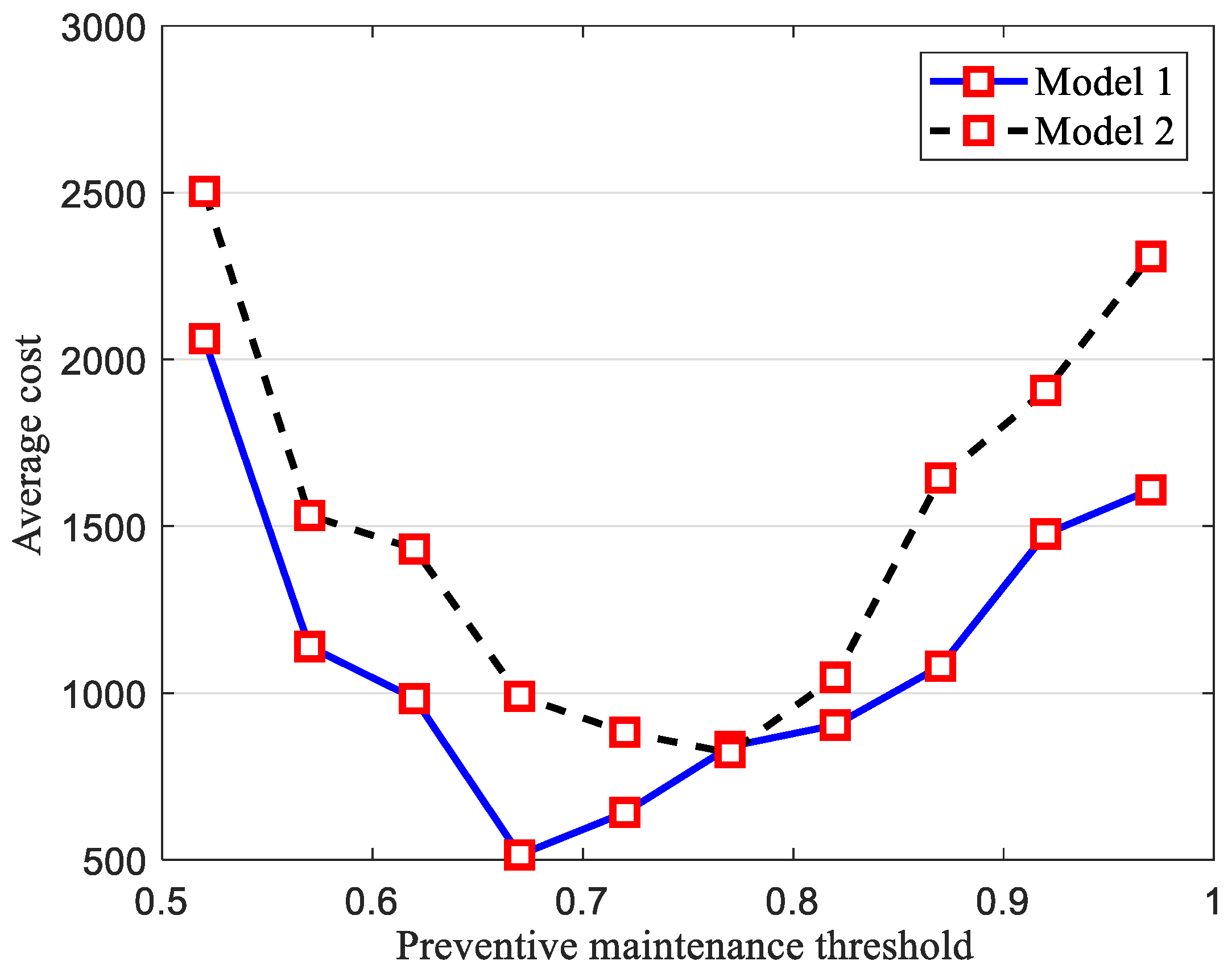
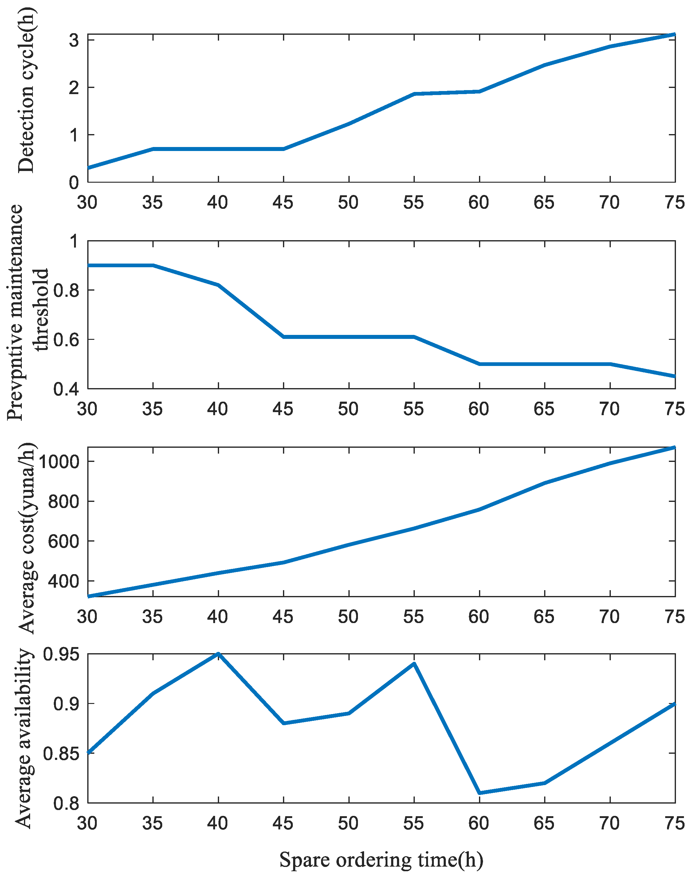
5.2.3. Comparative Experiments and Sensitivity Analysis

For Model 1 and Model 2, the detection period is set to $\Delta t=0.7$ h, and the aim is to compare the impact of the preventive maintenance threshold on the average cost. It can be seen from Figure 12 that when $w_p=0.67$, the minimum average cost based on model 1 is 514.65 dollars/h. When $w_p=0.77$, the minimum average cost based on Model 2 is 820.61 dollars/h. By comparison, it is obvious that the average cost based on Model 1 is lower than that based on Model 2. The main reason is that Model 2 ignores the impact of imperfect maintenance activities on decision goals.

The following is the sensitivity analysis of decision variables and decision objectives for spare parts ordering time. Other parameters considered will affect the experimental analysis. This paper uses the fixed independent parameter method to study. Assuming that the interval of spare parts ordering time is kept at $[30,75]$, the sensitivity of detection period, preventive maintenance threshold, average cost and availability to spare parts ordering time are studied, respectively.

It can be seen from Figure 13 that when the spare parts ordering time changes, the availability is irregular, and we generally select the part with availability greater than 0.9. The average cost will increase with the increase of spare parts order time, because the increase of spare parts time will lead to the increase of spare parts order cost and downtime cost. The preventive maintenance threshold will decrease with the increase of spare parts ordering time, indicating that the longer the downtime, the more frequently maintenance will be required. The detection period maintains a positive correlation with the spare parts ordering time. The longer the spare parts ordering time is, the longer the downtime is, and the longer the detection period will be.

Based on the experimental analysis, it can be seen that the model in this paper jointly optimizes the average cost with the number of imperfect maintenance activities and availability as constraints. Finally, the optimal decision variables are obtained to achieve the optimal maintenance of the degraded equipment. At the same time, the influence of the change of spare parts order time on decision variables and decision criteria is analyzed. The results show that the average cost and the inspection cycle are positively correlated with the spare parts order time.

6. Conclusions

In this paper, aiming at the joint optimization problem of the maintenance strategy of nonlinear degraded equipment, a joint optimization strategy of the condition-based maintenance and spare parts ordering of nonlinear degradation equipment under imperfect maintenance was proposed. Based on the linearization ability of BCT for nonlinear degradation data, the RUL prediction information is obtained by combining the random coefficient regression model. Then the probability of successful execution of imperfect maintenance activities, preventive replacement and failure replacement is derived, and the joint optimization model is constructed. Finally, the feasibility of the method in this paper was verified by numerical simulation. The results show that the number of imperfect maintenance activities was more than that of direct analysis of the original degradation data through the analysis of the nonlinear degradation data after BCT, indicating that the proposed method can achieve the purpose of equipment life extension. At the same time, this paper determined the optimal detection cycle and preventive maintenance threshold needed to reduce the average maintenance cost of equipment under the premise of meeting the availability.

In addition, the proposed method provides some ideas for future research directions:

(1)

In this paper, the maintenance strategy of similar nonlinear degradation equipment was studied. In engineering practice, the research goal can be multivariate and systematic. Thus, it is necessary to construct a multivariate nonlinear degradation model and consider the uncertainty of imperfect maintenance activities of multivariate systems.

(2)

Considering the influence of parameters such as detection cost and maintenance cost on the joint optimization model, the joint optimization model can be optimized by combining decision variables.

References

1. Si, X.; Li, T.; Zhang, Q.; Hu, X. An Optimal Condition-based replacement method for systems with observed degradation signals. IEEE Trans. Reliab. 2018, 67, 1281–1293. [Google Scholar] [CrossRef]
2. Chen, C.; Lu, N.; Jiang, B. Condition-based maintenance optimization for continuously monitored degrading systems under imperfect maintenance actions. J. Syst. Eng. Electron. 2020, 31, 841–851. [Google Scholar]
3. Yan, T.; Lei, Y.; Wang, B.; Han, T.; Si, X.; Li, N. Joint maintenance and spare parts inventory optimization for multi-unit systems considering imperfect maintenance actions. Reliab. Eng. Syst. Saf. 2020, 202, 106994. [Google Scholar] [CrossRef]
4. Zhang, X.; Zeng, J. Joint Optimization of Condition-based Preventive Maintenance and Spare Parts Provisioning Policy for Equipment Maintenance. J. Mech. Eng. 2015, 51, 150–158. [Google Scholar] [CrossRef]
5. Cai, J.; Xiao, L.; Li, X. Joint optimization of maintenance decision and spare parts inventory based on Wiener process. Syst. Eng. Electron. 2016, 38, 1854–1859. [Google Scholar]
6. Jiang, Y.; Guo, T.; Zhou, D. Joint decision on replacement time and spare ordering time based on remaining useful life prediction. CIESC J. 2015, 66, 284–290. [Google Scholar]
7. Lu, N.; Chen, C.; Jiang, B.; Xing, Y. Latest Progress on Maintenance Strategy of Complex System: From Condition-based Maintenance to Predictive Maintenance. Acta Autom. Sin. 2021, 47, 1–17. [Google Scholar]
8. Pei, H.; Hu, C.; Si, X.S.; Zhang, Z.; Du, D. Remaining Life Prediction Information-based Maintenance Decision Model for Equipment Under Imperfect Maintenance. Acta Autom. Sin. 2018, 44, 719–729. [Google Scholar]
9. Deep, A.; Zhou, S.; Veeramani, D. A data-driven recurrent event model for system degradation with imperfect maintenance actions. IISE Trans. 2022, 54, 271–285. [Google Scholar] [CrossRef]
10. Xu, J.; Liang, Z.; Li, Y. Generalized condition-based maintenance optimization for multi-component systems considering stochastic dependency and imperfect maintenance. Reliab. Eng. Syst. Saf. 2021, 211, 107592. [Google Scholar] [CrossRef]
11. Wang, X.; Gaudoin, O.; Doyen, L.; Bérenguer, C.; Xie, M. Modeling multivariate degradation processes with time-variant covariates and imperfect maintenance effects. Appl. Stoch. Model. Bus. Ind. 2020, 37, 592–611. [Google Scholar] [CrossRef]
12. Sofiene, D.; Mohamed, N. An improved imperfect maintenance strategy for multiperiod randomly failing equipment with stochastic repair times. J. Qual. Maint. Eng. 2022, 28, 491–505. [Google Scholar]
13. Zhang, N.; Yu, C.; Xie, F. The time-scaling t-ransformation technique for optimal control problems with time-varying time-delay switched systems. J. Oper. Res. Soc. China 2020, 8, 581–600. [Google Scholar] [CrossRef]
14. Yang, Z.; Teng, W.; Duan, Z.; Zhang, J. Reducing forecast errors by logarithmic transformations for complex time series. In Proceedings of the 2012 2nd International Conference on Consumer Electronics, Communications and Networks (CECNet), Yichang, China, 21–23 April 2012; pp. 2761–2764. [Google Scholar]
15. Pang, G.; Liu, J.; Liu, J.; Guo, Y.; Yian, X. Study on the decision considering imperfect maintenance of multiple components based on the exponential distribution. J. Phys. Conf. Ser. 2020, 1437, 012098. [Google Scholar] [CrossRef]
16. Wang, Z.; Chen, Y.; Cai, Z.; Wang, L.; Xiang, H. Optimal replacement strategy considering equipment remaining useful lifetime prediction information under the influence of uncertain failure threshold. J. Natl. Univ. Def. Technol. 2021, 43, 145–154. [Google Scholar]
17. Wu, F.; Niknam, S.A.; Kobza, J.E. A cost effective degradation-based maintenance strategy under imperfect repair. Reliab. Eng. Syst. Saf. 2015, 144, 234–243. [Google Scholar] [CrossRef]
18. Zhou, S.; Tang, Y.; Xu, A. A generalized Wiener process with dependent degradation rate and volatility and time-varying mean-to-variance ratio. Reliab. Eng. Syst. Saf. 2021, 216, 107895. [Google Scholar] [CrossRef]
19. Zhang, C.; Qi, F.; Zhang, N.; Li, Y.; Huang, H. Maintenance policy optimization for multi-component systems considering dynamic importance of components. Reliab. Eng. Syst. Saf. 2022, 226, 108705. [Google Scholar] [CrossRef]
20. Li, T.; Si, X.; Liu, X.; Pei, H. Data-model interactive remaining useful life prediction technologies for stochastic degrading devices with big data. Acta Autom. Sin. 2021, 48, 2119–2141. [Google Scholar]
21. Wu, Y.; Yang, Z.; Wang, J.; Chen, X.; Hu, W. Optimizing opportunistic preventive maintenance strategy for multi-unit system of CNC lathe. J. Mech. Sci. Technol. 2022, 36, 145–155. [Google Scholar]
22. Box, G.; Cox, D.R. An analysis of transformations. J. R. Stat. Soc. Ser. B Methodol. 1964, 78, 211–252. [Google Scholar] [CrossRef]
23. Guo, C.; Wang, W.; Guo, B.; Si, X. A maintenance optimization model for mission-oriented systems based on Wiener degradation. Reliab. Eng. Syst. Saf. 2013, 111, 183–194. [Google Scholar] [CrossRef]
24. Pang, Z.; Pei, H.; Li, T.; Hu, C.; Si, X. Remaining useful lifetime prognostic approach for stochastic degradation equipment considering imperfect maintenance activities. J. Mech. Eng. 2022, 58, 1–16. [Google Scholar]
25. Si, X.; Wang, W.; Hu, C.; Hu, C.; Chen, M.; Zhou, D. A Wiener process based degradation model with a recursive filter algorithm for remaining useful life estimation. Mech. Syst. Signal Process. 2013, 35, 219–237. [Google Scholar] [CrossRef]
Figure 1. Degradation trajectory of nonlinear degraded equipment under imperfect maintenance.
Machines 10 01041 g001
Figure 2. Preparation of state degradation and maintenance process.
Machines 10 01041 g002
Figure 3. Preventive replacement and spare parts ordering process 1.
Machines 10 01041 g003
Figure 4. Preventive replacement and spare parts ordering process 2.
Machines 10 01041 g004
Figure 5. Failure replacement and spare parts ordering process 1.
Machines 10 01041 g005
Figure 6. Failure replacement and spare parts ordering process 2.
Machines 10 01041 g006
Figure 7. Degradation trajectory before and after BCT.
Machines 10 01041 g007
Figure 8. Probability of successful execution of imperfect maintenance activities.
Machines 10 01041 g008
Figure 9. Probability of fourth imperfect maintenance to different levels.
Machines 10 01041 g009
Figure 10. Relationship between variables of joint optimization model and average cost.
Machines 10 01041 g010
Figure 11. Relationship between variables and availability of joint optimization model.
Machines 10 01041 g011
Figure 12. Comparison of average cost of two models.
Machines 10 01041 g012
Figure 13. Relationship between spare order time and decision variables, decision criterion.
Machines 10 01041 g013