Article

Experimental Fatigue Evaluation of Bogie Frames on Metro Trains

1
School of Traffic & Transportation Engineering, Central South University, Changsha 410075, China
2
Key Laboratory of Traffic Safety on Track (Central South University), Ministry of Education, Changsha 410075, China
3
Joint International Research Laboratory of Key Technology for Rail Traffic Safety, Central South University, Changsha 410075, China
4
National & Local Joint Engineering Research Center of Safety Technology for Rail Vehicle, Changsha 410075, China
5
China Railway Rolling Stock Corporation Qingdao Sifang Co., Ltd., Qingdao 266111, China
*
Author to whom correspondence should be addressed.
Machines 2022, 10(11), 1003; https://doi.org/10.3390/machines10111003
Submission received: 6 October 2022 / Revised: 23 October 2022 / Accepted: 28 October 2022 / Published: 31 October 2022

Abstract

:
Metro vehicles have always been known for their high passenger density, frequent traffic flow and strong alternating loads due to their severe running environment. As the major support component, the bogie frame suffers from fatigue damages and receives a high intensity of interest. In this work, a theoretical model is presented between the measured strain and the structural stress via multiple load identification, wherein recognition matrices and stress evaluations of the bogie frame are defined according to the locations found in finite element analysis (FEA). The model is validated through random loading in FE simulation, and the load deviation is within 1.1 kN. A vehicle experiment was performed on the second bogie of the head car on a six-car metro train. The signed von Mises (SVM) stress was calculated at critical locations with the proposed method and compared with what was measured. The excessive part was no more than 14.97%, comparing the reconstructed with the measured amounts. Stress spectra were developed utilizing rain-flow counting and evaluated in terms of the damage accumulation rule with the optimal spectra groups determined from convergence analysis. The evaluation indicates that, when the running mileage increases to the full life cycle of 3,960,000 km, the maximum equivalent damage reaches 0.35 and 0.46 at the gear box base for measured and reconstructed amounts, respectively. Research outcomes suggest that the proposed method offers an alternative for fatigue assessment and maintenance strategies on metro vehicles, as well as other types of rail-transit vehicles.

1. Introduction

Metro systems aim to provide safe, reliable, accessible and friendly public transportation services in a city. But for metro lines in big cities like Beijing and Guangzhou, huge passenger flows bring about a high full-load ratio and lengthy, overcrowded travel, which gives rise to the long-term overload operation of the metro train. Unlike high-speed trains, the loading on metro vehicles often exceeds the AW3 scenario during peak times, in which the assigned weight includes seated plus six standing passengers per square meter [1]. The consistent overloading raises the risk of fatigue failure on key support structures, as the load enhances in both amplitude and cycle numbers [2,3,4,5]. Hence, to better understand the fatigue behavior of vehicle structure, a vehicle test is the best way to assess the practical stress response and estimate the potential weakness [6,7,8,9,10].
To provide an effective and exact evaluation of the fatigue damage state of rail vehicle operation, measurement point selection, load identification and fatigue life assessment methods are required to ensure the validity of the assessment. Commonly used methods for fatigue assessment are numerical simulations and vehicle tests. Numerical simulation analysis mainly involves the selection of fatigue load conditions, the modeling of the structural specifications on the vehicle and the establishment of stress assessment criteria [11,12,13]. In experiments, the acquisition of realistic stress input data is a prerequisite for subsequent accurate fatigue assessment [14].
Rail vehicles are subjected to random dynamic loads during operation, so they have a more complex load status than conventional vehicles, and the fatigue numerical simulation method is broadly used due to their short development cycle and strong competitive edge [15]. Lu [16] adopted the inherent strain method to numerically simulate the welding deformation of the frame, then analyzed the stress state under the standard load and modeling method for the bogie frame, based on the basic theory of multi-axial fatigue strength. Miao [17] proposed a systematic method to simulate the fatigue life of vehicle-body structures by using a combination of multi-body dynamics simulation and FEA; moreover, a time–frequency conversion algorithm for orbital spectra was constructed to solve the spectral feature information lost during conversion by conventional methods. The condition of random vibration has also been studied through a comparison of dynamic model simulation and testing, and the results indicate that Dirlik’s and Steinberg’s models can support exact results for fatigue failure prediction [18].
Correct evaluation of the maximum structural stress may considerably increase the accuracy of failure assessment and prediction [19,20,21]. However, the internal stress data of the structure cannot be measured by the traditional sensor method, and various approaches have been developed for reconstructing the structural stress. H.E. Coules [22] carried out the reconstruction with two techniques, inferred the complete state of residual stress [23] from a limited set of experimental measurements and used finite element analysis to compare and show an exact reconstruction of the stress field. Toshiya Nakamura used the complex stress functions given by the finite series of polynomials [24], then found the proper set of coefficients required to make the best fit to the strain data and demonstrated that the present method reconstructed the stress field around the hole and that the estimated stress agreed with the FEA result. Since the irregular load input in design specifications could not fully meet the actual operating conditions, Wang [25] developed a long-term test of the high-precision dynamometric frame to obtain the real loading conditions, achieving the fatigue reliability improvement comprehensively.
Fatigue life estimation goes beyond what is measured during the vehicle test, if the reconstructed stress at hard-to-measure locations gives a more conservative evaluation. In this work, theoretical modeling is presented in Section 2 to find mechanical relations between external loads and strain captures. The identified loads are then used to obtain the structural stress at critical locations. In Section 3, the theoretical model is applied and calibrated on the bogie frame by FE simulation, wherein the load identification and stress calculation matrix are fitted under an individual load case in its load limit. Simulation validation undergoes 10 random coupled load cases in comparison between the given and identified loads. In Section 4, a vehicle test is conducted on a 6-car metro train to acquire the strain measurement. Fatigue evaluation is given in terms of both measured and reconstructed stress spectra. The framework of this paper is shown in Figure 1.

2. Theoretical Modeling

2.1. Strain Capture

For loaded structures, external loads are defined as F1, F2, … FN at N locations. Those loads act in terms of concentrating forces at connections or uniform loads at the contact interface. For each kind, the load limit is denoted as F1MAX, F2MAX, … FNMAX, respectively. To recognize all external loads, N strain captures are required to create the equations capable of correlating the resultant strain responses and acting forces.
Strain capture is located at the structural face on node or element where large surface strain occurs under a relating load case. Capture locations are labeled as L1#(SURF), L2#(SURF), … LN#(SURF) when subjected to pure load F1, F2, … FN, respectively. In each load case, a linear relationship can be observed between the captured strain and acting load in Equation (1) as below during the material elastic stage.
ε F 1 L 1 ( SURF ) = C F 1 L 1 ( SURF ) · F 1 , ε F 2 L 1 ( SURF ) = C F 2 L 1 ( SURF ) · F 2 , ε FNL 1 ( SURF ) = C FNL 1 ( SURF ) · F N ε F 1 L 2 ( SURF ) = C F 1 L 2 ( SURF ) · F 1 , ε F 2 L 2 ( SURF ) = C F 2 L 2 ( SURF ) · F 2 , ε FNL 2 ( SURF ) = C FNL 2 ( SURF ) · F N ε F 1 LN ( SURF ) = C F 1 LN ( SURF ) · F 1 , ε F 2 LN ( SURF ) = C F 2 LN ( SURF ) · F 2 , ε FNL 2 ( SURF ) = C FNL N ( SURF ) · F N
where εF1L1(SURF), εF2L1(SURF), …εFNL1(SURF) are the strain at L1#(SURF) when subjected to pure load F1, F2, … FN, respectively. CF1L1(SURF), CF2L1(SURF), …CFNL1(SURF) are the coefficient between the strain at L1#(SURF) and the pure load F1, F2, … FN, respectively, which can be obtained through FE simulation in single loading. For other strain captures and acting loads, parameters are defined according to the same rule as the strain at L1#(SURF).

2.2. Load Identification

In practical circumstance, the captured surface strain is composed of the strain responses from each load, which yields
ε L 1 ( SURF ) = ε F 1 L 1 ( SURF ) + ε F 2 L 1 ( SURF ) + ε FNL 1 ( SURF ) ε L 2 ( SURF ) = ε F 1 L 2 ( SURF ) + ε F 2 L 2 ( SURF ) + ε FNL 2 ( SURF ) ε LN ( SURF ) = ε F 1 LN ( SURF ) + ε F 2 LN ( SURF ) + ε FNLN ( SURF )
where εL1(SURF), εL2(SURF), …εLN(SURF) are the surface strain at L1#(SURF), L2#(SURF), …LN#(SURF), respectively.
All captured strains can be given in matrix form according to Equations (1) and (2) as below.
{ ε L 1 ( SURF ) ε L 2 ( SURF ) ε LN ( SURF ) } = [ C F 1 L 1 ( SURF ) C F 2 L 1 ( SURF ) C FNL 1 ( SURF ) C F 1 L 2 ( SURF ) C F 2 L 2 ( SURF ) C FNL 2 ( SURF ) C F 1 LN ( SURF ) C F 2 LN ( SURF ) C FNLN ( SURF ) ] · { F 1 F 2 F N }
External loads can therefore be given by the inversion of Equation (3) in Equation (4).
F 1 F 2 F N = C F 1 L 1 ( SURF ) C F 2 L 1 ( SURF ) C FNL 1 ( SURF ) C F 1 L 2 ( SURF ) C F 2 L 2 ( SURF ) C FNL 2 ( SURF ) C F 1 LN ( SURF ) C F 2 LN ( SURF ) C FNLN ( SURF ) 1 · ε L 1 ( SURF ) ε L 2 ( SURF ) ε LN ( SURF ) = M IDF · ε L 1 ( SURF ) ε L 2 ( SURF ) ε LN ( SURF )
The identification matrix from surface strain to loads is denoted as MIDF as above.

2.3. Stress Reconstruction

Stress evaluation occurs at the structural node or element where large structural stress occurs under relating load case. Different from strain capture locations, structural stress might appear in internal region or positions that are infeasible to place strain gauges in. To distinguish stress evaluation positions from strain capture, evaluation locations are labeled L1#(STRU), L2# (STRU), … LN# (STRU) when subjected to pure load F1, F2, … FN, respectively. In a full load case, when all loads act to limits concurrently, the large stress node/element position is denoted as ALL#(STRU).
For (N+1) stress evaluation points, the 6-component structural stress is composed of the stress caused by each load case at the evaluation point, respectively. Therefore:
σ L 1 ( STRU ) = σ F 1 L 1 ( STRU ) + σ F 2 L 1 ( STRU ) + σ FNL 1 ( STRU ) σ L 2 ( STRU ) = σ F 1 L 2 ( STRU ) + σ F 2 L 2 ( STRU ) + σ FNL 2 ( STRU ) σ LN ( STRU ) = σ F 1 LN ( STRU ) + σ F 2 LN ( STRU ) + σ FNLN ( STRU ) σ LALL ( STRU ) = σ F 1 LALL ( STRU ) + σ F 2 LALL ( STRU ) + σ FNLALL ( STRU )
where σL1(STRU), σL2(STRU) … σLN(STRU) and σLALL(STRU) are the 6-component structural stress at (N+1) evaluation locations respectively. σF1L1(STRU), σF2L1(STRU), …σFNL1(STRU) are the 6-component stress at L1#(STRU) when subjected to pure load F1, F2, … FN, respectively. For other stress evaluation positions and acting loads, parameters are defined in the same rule as the stress at L1#(STRU).
Formula (5) can be expressed in matrix form correlating 6-component stress with external loads in Equation (6) as below.
σ L 1 ( STRU ) σ L 2 ( STRU ) σ LN ( STRU ) σ LALL ( STRU ) = C F 1 L 1 ( STRU ) C F 2 L 1 ( STRU ) C FNL 1 ( STRU ) C F 1 L 2 ( STRU ) C F 2 L 2 ( STRU ) C FNL 2 ( STRU ) C F 1 LN ( STRU ) C F 2 LN ( STRU ) C FNLN ( STRU ) C F 1 LALL ( STRU ) C F 2 LALL ( STRU ) C FNLAL ( STRU ) F 1 F 2 F N = M RCS · F 1 F 2 F N
where CF1L1(STRU), CF2L1(STRU), …CFNL1(STRU) are the coefficients between 6-component stress at L1#(STRU) and the pure load F1, F2, … FN, respectively, which can be acquired through FE simulation in single loading. For other stress evaluation positions and acting loads, parameters are defined in the same rule as the structural stress at L1#(STRU). The reconstruction matrix from load to structural stress is denoted as MRCS.
According to Equations (4) and (6), the theoretical model of structural stress reconstruction at (N+1) evaluation positions can be obtained by calculating the captured strain of N monitoring points in Equation (8) as below.
σ L 1 ( STRU σ L 2 ( STRU ) σ LN ( STRU ) σ LALL ( STRU ) ( i ) = C F 1 L 1 ( STRU ) C F 2 L 1 ( STRU ) C FNL 1 ( STRU ) C F 1 L 2 ( STRU ) C F 2 L 2 ( STRU ) C FNL 2 ( STRU ) C F 1 LN ( STRU C F 2 LN ( STRU ) C FNLN ( STRU ) C F 1 LALL ( STRU ) C F 2 LALL ( STRU ) C FNLALL ( STRU ) ( i ) · C F 1 L 1 ( SURF ) C F 2 L 1 ( SURF ) C FNL 1 ( SURF ) C F 1 L 2 ( SURF ) C F 2 L 2 ( SURF ) C FNL 2 ( SURF ) C F 1 LN ( SURF ) C F 2 LN ( SURF ) C FNLN ( SURF ) 1 · ε L 1 ( SURF ) ε L 2 ( SURF ) ε LN ( SURF ) = M RCS ( i ) · M IDF · ε L 1 ( SURF ) ε L 2 ( SURF ) ε LN ( SURF ) ,
where (i) represents the 6-components’ stress respectively. Hence, the standard von Mises stress [26] is calculated as Equation (8).
σ V M = 1 2 [ ( σ x σ y ) 2 + ( σ y σ z ) 2 + ( σ x σ z ) 2 + 6 ( τ x y 2 + τ y z 2 + τ x z 2 ) ]
where σx, σy, σz, τxy, τyz, τzx represent the normal stress along the x, y, z directions and the shear stress in xy, yz, and zx planes, respectively.
The standard von Mises stress is a poor choice for fatigue evaluation because the range calculated does not include any potentially negative part of the stress cycle. The signed von Mises stress (SVM), which takes the negative values, is therefore given by Equation (9) as the stress calculation rule.
σ SVM = sign ( I 1 ) · σ VM
where I1 is the first stress invariant, I1 = σx+ σy+ σz. Function sign() values +1 if I1 is positive, and −1 if I1 is negative.

3. FE Simulation on Metro Bogie Frame

Bogie frames serve as an important component in load transmission, passenger carrying and wheelset fixing. After a long period of operation, the bogie frame is one of the components most likely to suffer fracture or failure due to severe alternating loads. In this part, the bogie frame of a metro vehicle is investigated, adopting the above theoretical model in load identification and stress reconstruction. The finite element modeling, strain capture, determination of coefficient matrix of load identification and stress reconstruction will be respectively presented on a bogie frame. Results will be validated, and the captured and reconstructed stress will be compared.

3.1. Model Description

The bogie frame is a steel welded structure composed of side beams, crossbeams and component mounting bases for air spring, primary suspension, etc. In FE modeling, a coordinate system is created to define boundary and load conditions, wherein the X-axis describes the longitudinal running direction, the Y-axis is parallel to the geometric axis of the wheel axle and the Z-axis is perpendicular to the ground. The mechanical properties of the bogie frame is listed in Table 1 as below.
The FE frame model is meshed with the C3D10 tetrahedral element in ABAQUS (Version 2020, Dassault Systèmes Simulia Corp., Johnston, RI, USA) to adapt to its complex shape. The average mesh size is set to 8 mm. The final FE model comprises 3,250,000 nodes and 1,840,000 elements, wherein the refined grid is meshed at loading parts including the shaft neck center and air spring mounting base. Due to the large-scale element size, parallelization was done with the computer workstation (AMD EPYC 7702 64-Core @ 2.20 GHz, 480 GB RAM) for enhanced computing speed. Underneath the bogie frame, the primary spring is simulated by the spring element (SPRING2) above the axle box, the stiffness of which is 850, 3700 and 4700 N mm−1 in the vertical, horizontal and longitudinal directions, respectively. The axle is simulated by the beam element (B31) in the tube section, the material property of which is defined the same as the practical axle. Portion parts are connected by welding in HYPERMESH (Version 2020, Altair Engineering, Inc., The GNU General Public License); to emulate the weld shape and stress distribution at the weld position accurately, solid units are used to simulate the weld. According to HG20580~20585-2011 standard [27], the welding electrode grade is selected as J507, and its material properties are shown in Table 2.
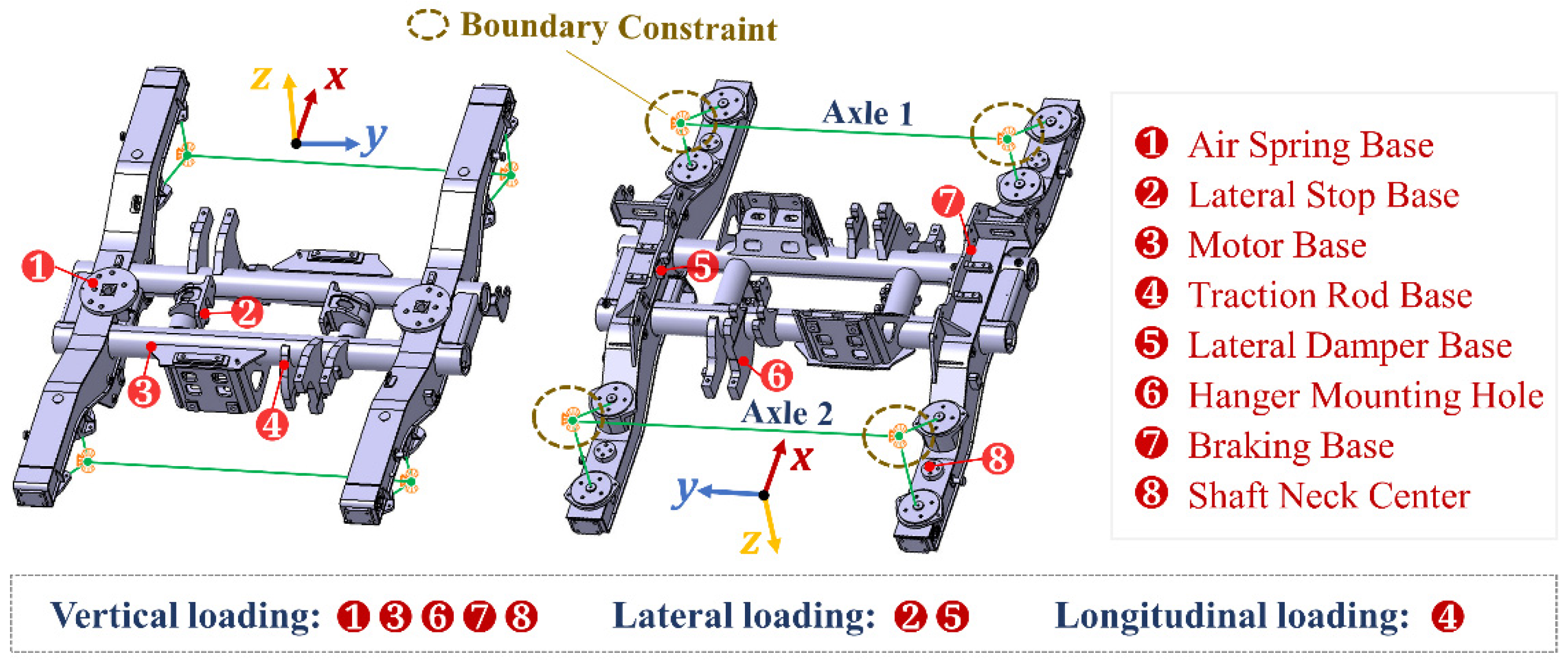
The boundary constraint is applied at the four shaft neck centers of two axles, as seen in Figure 2. In vertical load cases, longitudinal translation freedom along the x-axis is released at the shaft neck centers of axle 2#. All rotation freedoms are released at the shaft neck center of axle 1# and axle 2#, and other translation freedoms are constrained at the shaft neck centers. In longitudinal load cases in a running direction, rotation freedoms are released at all shaft neck centers, while other freedoms are all constrained. In lateral loading cases, full constraints are applied at four shaft neck centers.
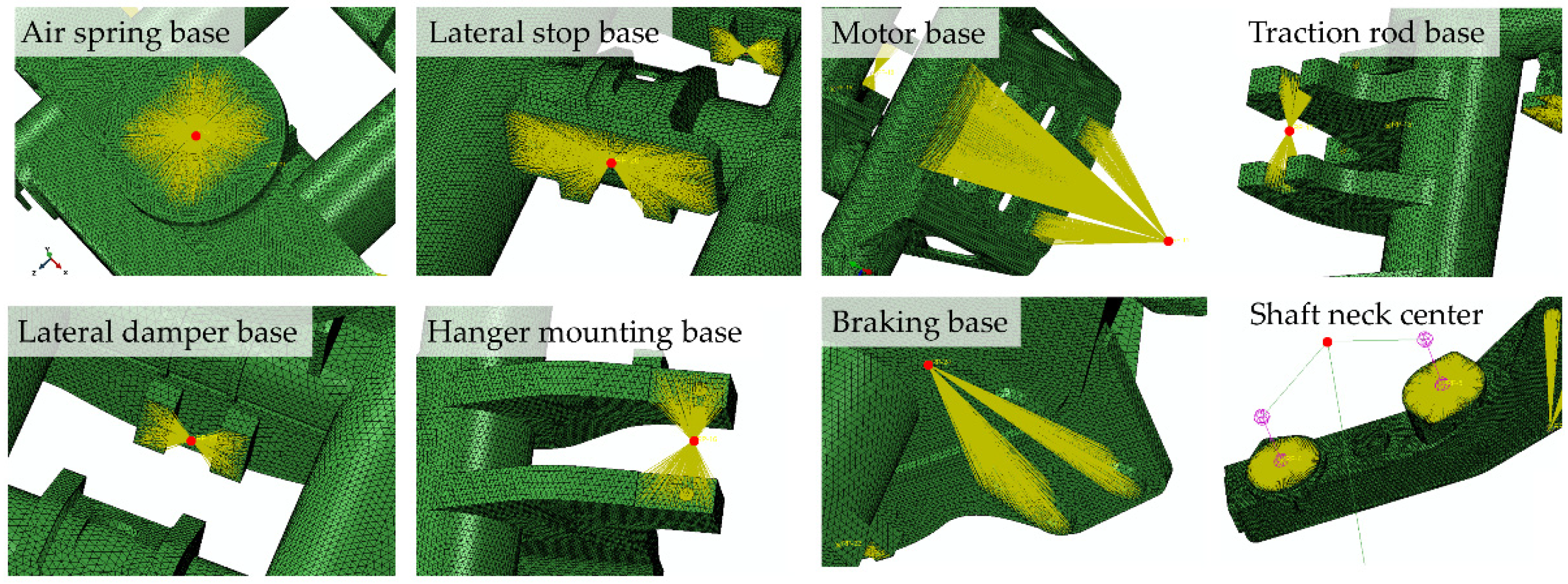
The loading conditions are categorized into 14 load cases according to TB/T CODE 2368-2005 on the motive power units, bogies and running gear and bogie frame structure strength tests [28]. In the simulation, reference points are established to couple the surfaces where loadings act; the loadings are applied on red reference points, as depicted in Figure 3. Load limits, positions and directions are defined in Table 3 to cover all possible load scenarios in contribution to structural strain and stress responses. The left and right direction is described in the bottom view in the running direction to distinguish the loading component positions. The positive lateral loading is from the left to the right, and the positive vertical loading is above the ground.

3.2. Scheme on Capture and Assessment

In FE simulation, each load case is performed to find a sensitive position on the frame surface suitable for strain gage bonding. The surface strain is read along the coordinate axis when the surface is parallel to the coordinate plane. When the plane is curved or inclined, the strain is read along a given path defined by the nodes at the critical zone, which is also the optimal path for strain-gauge placement. During the simulation of each load case, the von Mises stress is analyzed to detect the critical assessment positions, as stated in Section 2, in an attempt to reconstruct the equivalent stress from the identified loads.
After the simulation of each load case in its load limit, the strain capture locations and stress assessment positions are recognized and described in Table 4 as below.
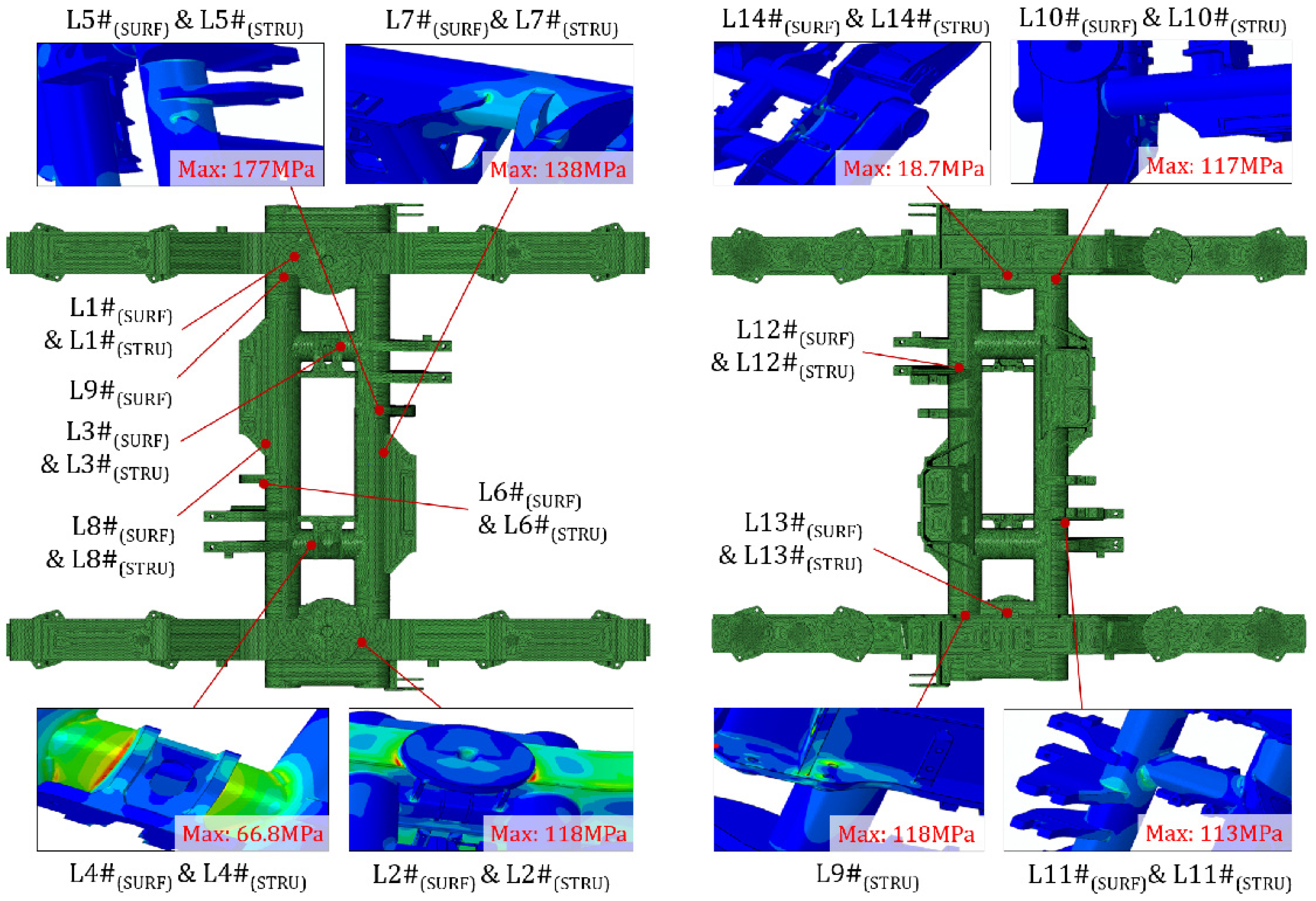
From the FE simulation results, the contour plots of structural stress are given in different load cases in Figure 4, and the maximum stresses are obtained under corresponding single-limit loads. The surface strain captures and structural stress assessment locations are indicated in Table 3.
As revealed from the above simulation, maximum strain and stress concentrate on the welding seam, based on simulation results. Evaluation points were selected by the maximum structural stress position suffering from 14 pure loading cases and 15 combined full loading cases, of which the large stress value point of the structure under the full loading case coincides with the large stress value point under LC5#. Considering the original defects and stress concentration in welding joints, fatigue damage easily occurs, and the capture location was selected to optimize the point layout strategy and to focus on the location of the weld. In this work, a strain gauge was used to measure the strain. Capture points L1#(SURF)~ L14#(SURF) were located according to maximum structural stress positions, among them, the L4#(SURF) capture point coincided with the point of structural maximum stress, as shown in Table 3.

3.3. Calculation on Identification and Reconstruction

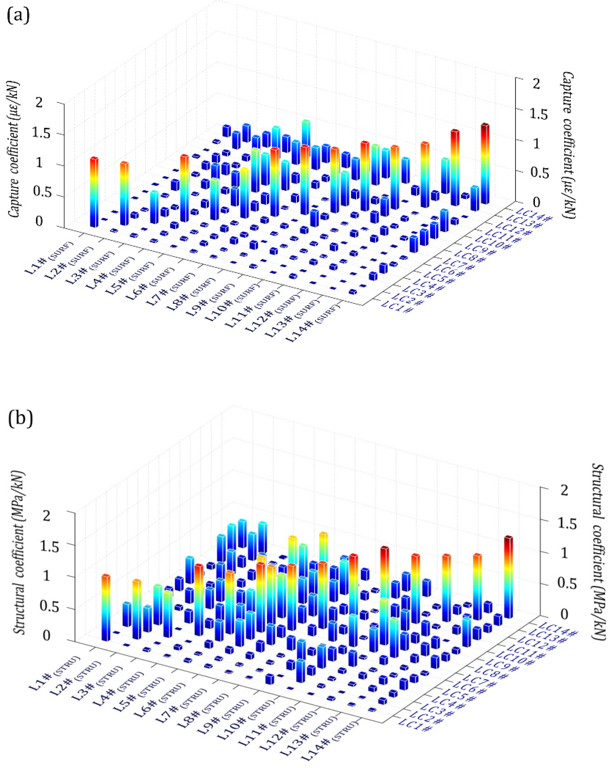
In the 14 load cases, each load limit was grouped into four grades, among which the zero loading was not included. After simulation in each sub-load case, surface strain responses at all captures and the 6-component stress at all assessment locations are read and fitted with corresponding load magnitudes. The identification coefficient, which is the ratio of the captured strain and the acting load, is given in a contour bar plot in Figure 5a. The reconstruction coefficient, which is the ratio of the von Mises stress and acting load, are given in the contour bar plot in Figure 5b.
As seen above, large coefficients appear in the diagonal region where the strain capture locations and stress assessment positions are determined according to their dominant load cases. In the second plot, the reconstruction coefficient of the von Mises stress from an identified load is, as stated in Equation (7), composed of the 6-component stress because the square root calculation of the von Mises stress no longer follows a linear relation with the identified loads as the stress component does. Thus, we have one 14 × 14 load identification matrix MIDF and six 14 × 14 stress reconstruction matrices MRCS(i) (i = 1~14) to realize load and stress recognition based on the measured surface strain at the 14 locations.

3.4. Validation on Load Identification

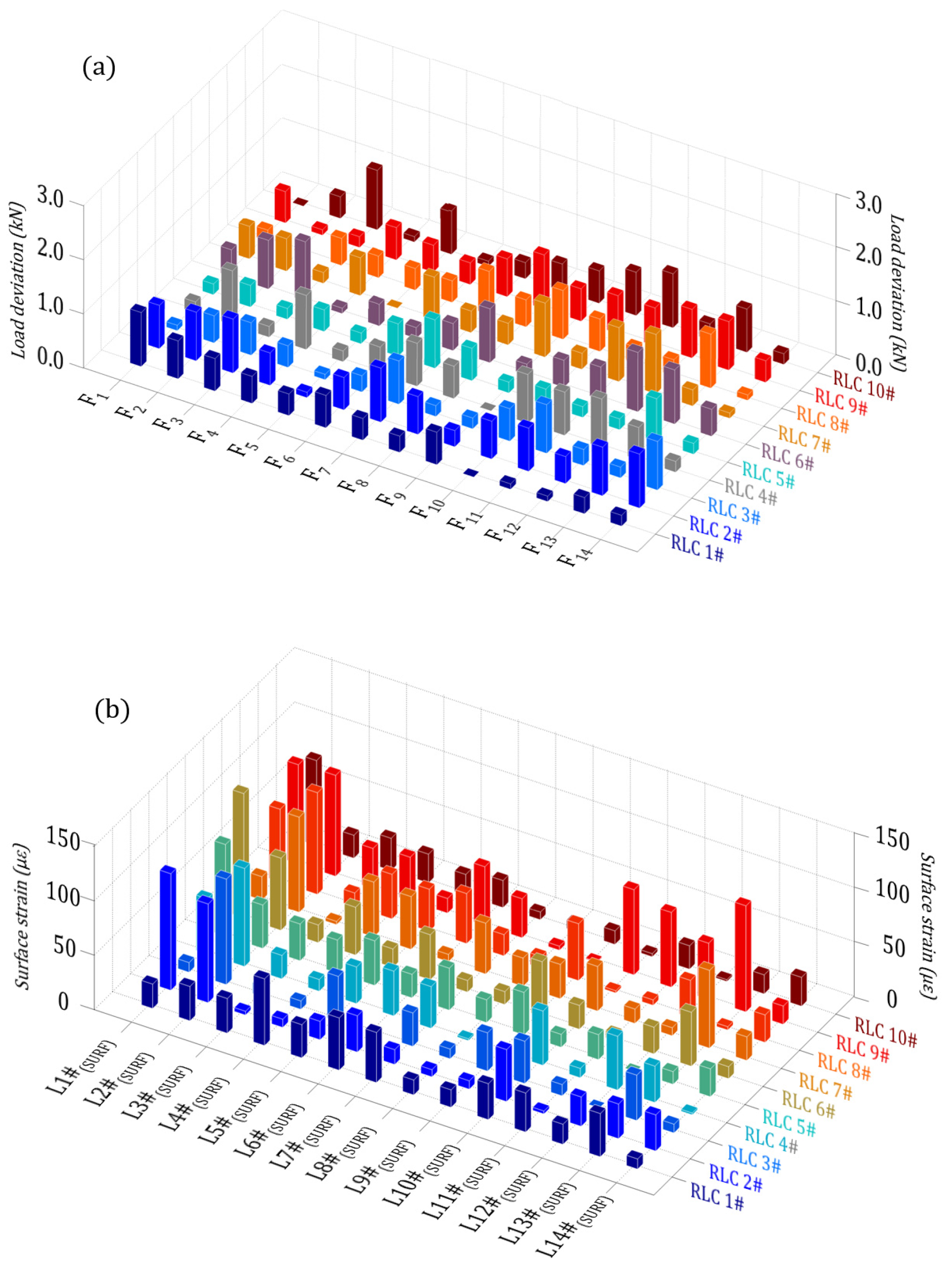
Validation for the proposed approach undergoes FE simulation by coupled random loading. In each random load case (abbreviated to ‘RLC’), the load magnitude is calculated by the product of the load limit and the random function. The load limit Fi(max) is defined in Table 3 for each load type, and the random function rand() varies from –1.0 to 1.0. To cover all possible coupling load circumstances, 10 different load cases are randomly generated in Table 5, denoted as given loads (labeled as ‘GV’). In each random load case, all loads concurrently act on the positions defined in Table 3. In the simulation solution, strains at the 14 capture locations are read and substituted into the load identification model in Equation (4). The identified load magnitudes for each type (denoted as ‘ID’) are then compared with the given randomly generated loads in Table 5. The absolute difference between ‘ID’ and ‘GV’ is given in the contour bar plot in Figure 6a, and the relative strain contour bar plot is given in Figure 6b.
It can be seen in Table 4 that the load deviation varies within 1.1 kN, with good accuracy between the identified and given loads. Due to the large loading in L1#, the strain calculated from the ID and surface coefficient in L1# also shows a large value, as depicted in Figure 6b, which verified the validity of the identification method.

4. Fatigue Assessment

An experimental test was performed on a metro train to record the strain time-history at the capture locations of the bogie frame according to FE simulation. The tested strains were used to, on one hand, identify the loads and equivalent stress at the 14 positions; on the other hand, they served as the measured stress for fatigue evaluation in comparison with the reconstructed stress. Fatigue damage was calculated by adopting rain-flow counting and the accumulation damage rule and was further analyzed in different periods of days and seasons.

4.1. Experiment Overview

The vehicle test was performed on the Beijing metro line, which has been famous for its mass passenger flow and high carrying capacity, especially during morning peaks and festivals, as in Figure 7. The maximum running speed on this line is 80 km h−1. The metro train is a six-car train which has three trailer cars and three motor cars, as shown in Figure 8. According to the finite element analysis done before and the stress data measured by the bogie bench test, the driving motor is carried on the bogie frame of the motor car instead of the trailer car. Hence, the test bogie is selected at the tail of the second motor car because of the heavier loads in operation.
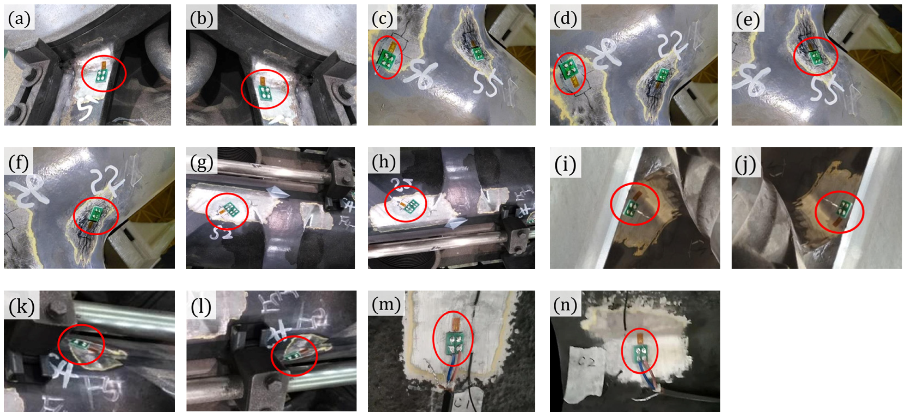
The full bridge resistance strain gauges from the German HBM company are bonded to the surface of the bogie frame at the 14 capture locations as mentioned in Section 3.2. The strain gages are arranged unidirectionally according to the vertical, lateral and longitudinal loads at different locations. They change resistance at their output terminals when getting stretched or compressed and compensate for the ambient temperature change by the dummy block where three other strain gauges are circuited in the Wheatstone bridge for each. The dummy block is installed near strain capture to share the same temperature sensation. As for data collection, the strain signal is collected through the IMC-C1 digital data acquisition system (DAQ) from the IMC company in Germany. The digital data acquisition terminal is installed at the “A” end of the vehicle and is hung on the vehicle underframe crossbeam using tooling, and the DC110V power cable is plugged into the terminal to supply power to the data acquisition system. DAQ is connected to the set-up computer for the monitoring, controlling and storage of the digital strain data. The sampling frequency is set to 5000 Hz because of the high alternative wheel–rail interaction responses, and a reasonable quality factor is selected for low-pass filtering [29]. Strain gauge locations are given in Figure 9 as below.
The vehicle test was performed for two months from August to October in 2019. The daily maximum running mileage was 602 km, and the total running mileage was 16,854 km. The daily mileage history during the test period is shown in Figure 10.
During experiment, the original strain data was collected and read into the load identification model found in Section 2.2 and further reconstructed into the von Mises stress shown in Section 2.3. The measured strain, identified loads and von Mises stress were analyzed and developed into load spectra in Section 4.3. The stress–strain conversion equation is shown in Equation (10), and the measured stress mentioned below is obtained by converting the measured strain based on Equation (10). Fatigue damage was assessed in suggested load spectra groups. Fatigue life was estimated based on measured strain, measured stress and reconstructed von Mises stress. The measured stress and measured strain yield are:
σ = E · ε
where σ, ε represent stress and strain, respectively, and E is the elastic modulus given in Table 1.

4.2. Results and Discussion

The peak stress at the capture locations of the bogie frame, which is defined as the maximum absolute stress calculated from the detected dynamic strain, is shown in Figure 11 for each day during the vehicle test period. The maximum stress occurs at the front gear box base (L11#(SURF)), which varies between 59.0 MPa to 74.3 MPa. The maximum peak arises on 29 September, when the train runs for 179.45 km. The minimum peak stress is located at the weld joints of the left air spring base (L2#(SURF)), which changes between 30.7 MPa to 35.7 MPa. All stress responses decreased on 1 October because of traffic restriction on the National Day.
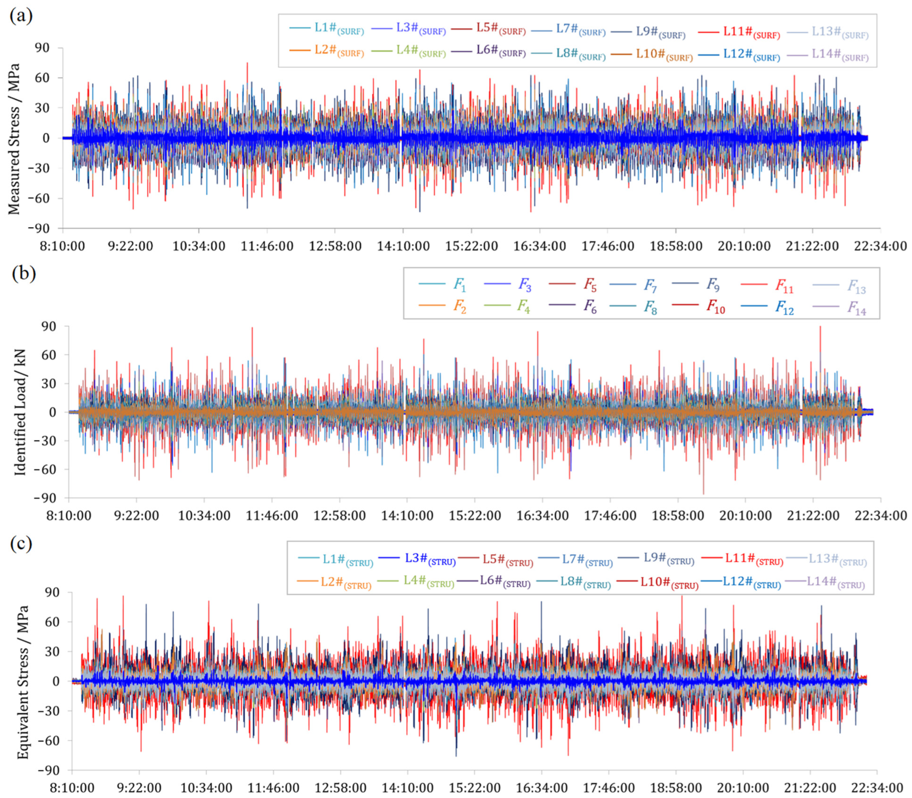
A detailed time-history of dynamic stress detection at 14 strain capture sites is given in Figure 12a on 29 September. By substituting the real-time strain captures in Equation (4), vertical, longitudinal and horizontal loads at facility mounting bases can be acquired, as in Figure 12b. The maximum loads are 92.9 kN, 85.9 kN and 61.3 kN for a vertical load at the front gear box base, a longitudinal load at the front traction rod base and a horizontal load at the right lateral stop base, respectively. The equivalent stress at evaluation locations is depicted in Figure 12c as below, where the peak stress reaches 39.5, 45.7, 57.2, 51.7, 80.5, 85.8 and 43.3 MPa for the left or right air spring base, left or right TLB, front or rear traction rod base, front or rear motor base, left brake base or right TSB, front or rear gear box base, left or right lateral damper base, respectively.
A bar plot of the peak stress, both measured and reconstructed, is given in Figure 13, from which it can be seen that the reconstruction peak stress is greater than the measured value, within 15% growth rates. Among them, the growth rates of L11#, L14# and L7# are 14.97%, 14.40% and 14.05%, respectively. The lowest is L12#, with a growth rate of 3.68%. Due to the superimposition of multiple load sources at L11#, the measured and reconstructed stress are highest in point 11, which is consistent with the actual operating conditions.
The results above indicate that the reconstructed stress is regularly stronger than the measured stress, which yields a more conservative evaluation compared to the conventional direct stress tests, but within 15% excess. Besides, this work performs a multi-point load identification method based on the full classification of bogie frame external loads, enabling the stress assessment of entire structures under full-scenario loading cases. Therefore, it is feasible to obtain the vehicle bogie frame operation status by stress field reconstruction, the method from which can also be applied to other circumstances wherein complex loads act on load-carrying structures in mechanical or other engineering areas.

4.3. Fatigue Damage Evaluation

Based on the stress time-history curves calculated above, the mean and amplitude load spectra in the full cycle are obtained by the rain-flow counting method, the principle of which is to determine a series of stress–strain hysteresis closed loops based on the nonlinear relationship between the measured material stress and strain, to simplify the actual measured load history into several load cycles, and to compile a stress-load spectrum for subsequent fatigue life estimation. After running the rain-flow counting program by MATLAB (R2014a), the mean and amplitude value in the full cycle of the time-history are obtained,
S m i = S i + S i + 1 2 ,     S a i = S i S i + 1 2  
where S is the load cycle, Smi is the mean stress load spectrum, Sai is the amplitude stress load spectrum, and it is a two-dimensional random process subject to a certain probability distribution. To calculate the fatigue life more precisely, the average value and amplitude of the stress cycle are grouped, and the statistics are carried out according to the frequency of each level,
G m = S m _ max + S m _ min m ,   G a = S a _ max S a _ min m  
where Gm is the load average grading group distance, m is the load grading number, and Sm_max and Sm_min are the maximum and minimum values of the mean load. Ga is the difference between the various levels of the amplitude stress load spectrum; Sa_max and Sa_min are the maximum and minimum values of the amplitude stress load spectrum.
Furthermore, the mean and amplitude values are graded to get a more stable cumulative damage. In this paper, Miner cumulative damage theory is used to evaluate the fatigue damage of the frame, that is, the damage increments caused by cyclic loading at each level under the action of a multistage variable amplitude fatigue load spectrum can be added independently. The damage caused by n cycles under variable amplitude load is
D = i 1 g n i N i  
where D is the cumulative fatigue damage of the material, g is the number of classifications, ni is the number of stress cycles under classification i, and Ni is the fatigue life. When the fatigue damage D = 1, the structure will be destroyed.
For the purpose of comprehensively considering the impact of load amplitude and average value, the Goodman life equation is used to convert all levels of loads into symmetrical cyclic loads, namely,
S 1 = S a S u S u S m  
where S−1 is the symmetric cyclic load amplitude, Sa is the load amplitude, Sm is the average load, Su is the ultimate strength of the material, and the 1-D load cumulative damage formula generated by a single 64-level stress spectrum is:
D = i 1 m N i s 1 ( i ) m c  
where m and c are the material constant of the S–N curve, Ni is the number of load cycles, and the cumulative damage formula of the 2-D load spectrum is:
D = i 1 m j 1 m N i j s 1 ( i , j ) m c  
where Nij is the number of load cycles. According to the cumulative damage criterion, Lall is the total operating mileage life, Dall is the total fatigue damage, Lcyc is the measured operating kilometers, and Dcyc is the measured fatigue, namely,
L all = D all L cyc D cyc
According to “JIS 4207 Railway Vehicle-Bogie-Bogie Frame Design General Standard”, the allowable fatigue stress of polished welds is 110 MPa, and other specific fatigue strength parameters are shown in Table 6.
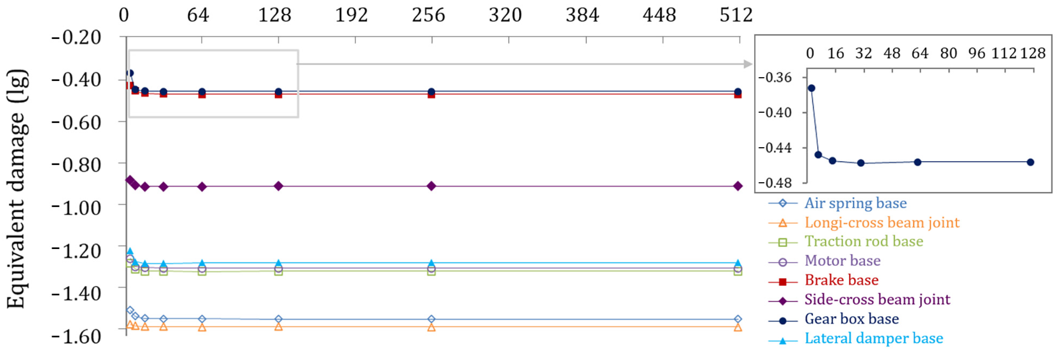
After the load spectrum classification reaches a certain value, the cumulative damage will reach a stable value, to obtain a reasonable grade of load spectrum. The logarithmic fatigue damage values of different grades for the eight positions are shown in Figure 14, where the gear box base weld L11# has the largest damage value; accordingly, L11# was selected to determine a reasonable grade for load spectrum. The equivalent damage reaches its maximum of 0.43 when the grade is 4 and gradually decreases as the grade increases, then maintains a stable value of 0.35 at grade 32. Therefore, the load spectrum grade in this paper is chosen as 32.
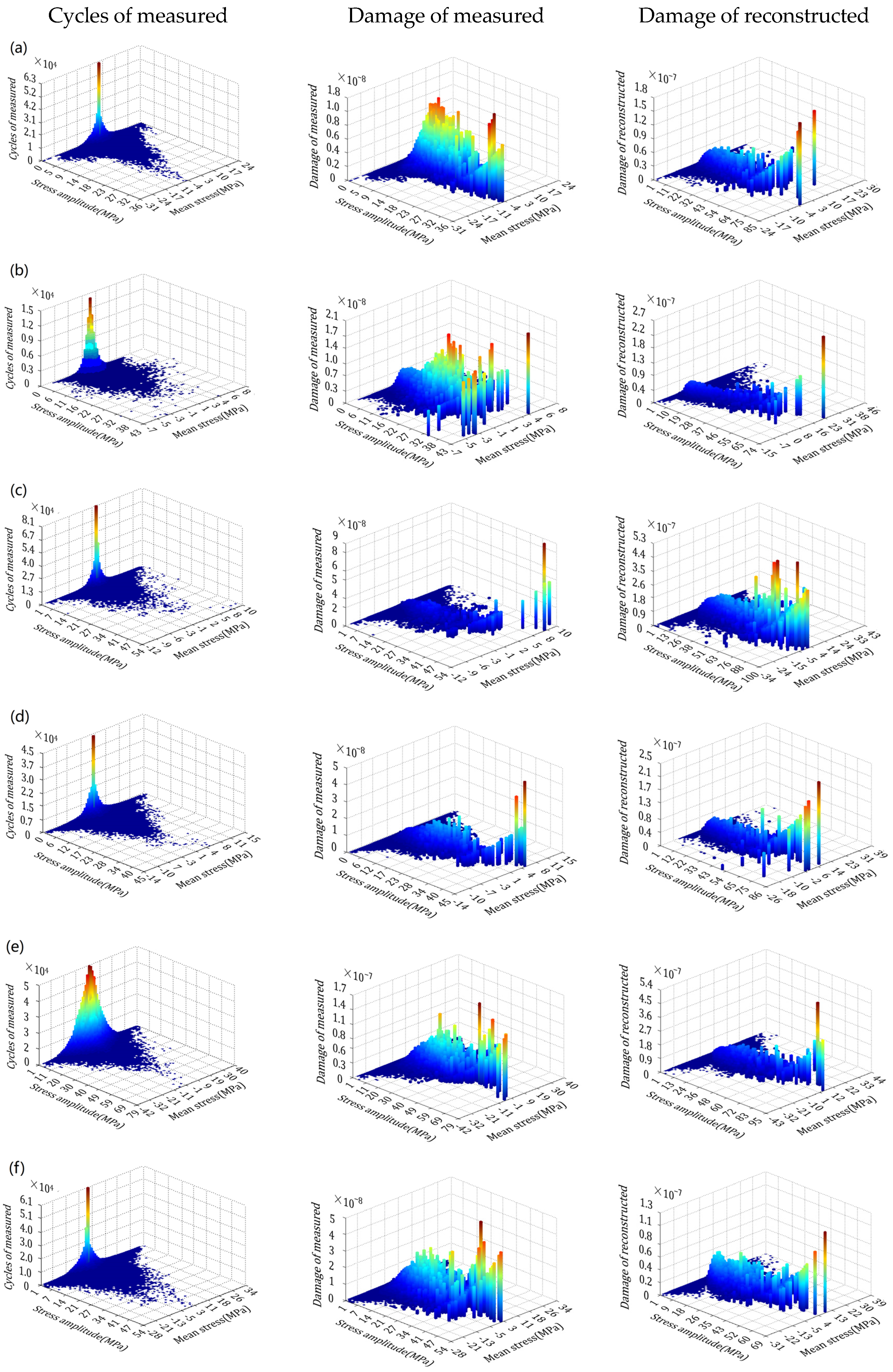
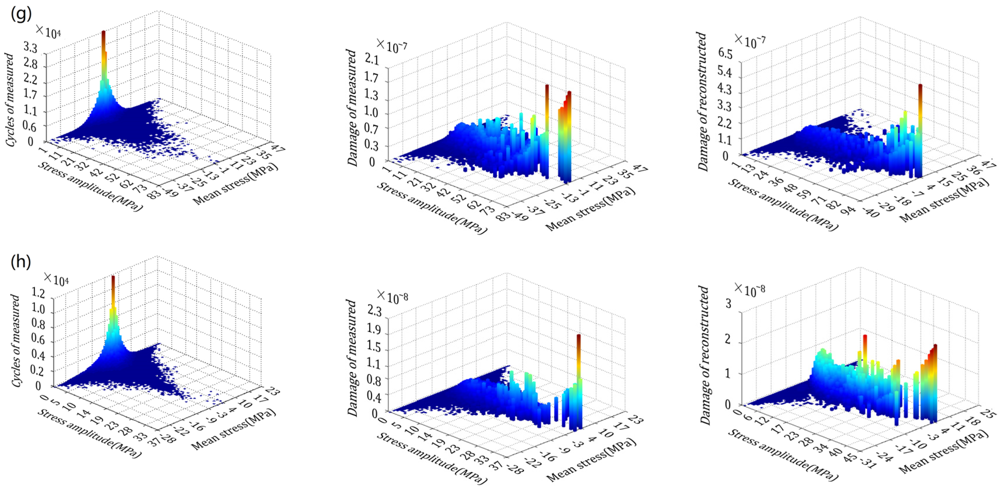
To further analyze the load distribution, the 32 grade 3-D mean and amplitude frequency diagrams of the captured stress and damage diagrams of captured and reconstructed stresses for eight load types were plotted, as in Figure 15.
As revealed in Figure 15, the distribution of load cycle counts is similar among the eight load types, but the highest cycle counts appear in L6#, and the lowest occur in L9#. The cycles of the measured spectrum are symmetrically distributed except for the L3#, and more than 95% mean load counts are concentrated within ±10 MPa. For the damage contour map, both measured and reconstructed damage are concentrated in the middle area of mean and amplitude stress, with a maximum measured damage of 1.5 × 10⁻⁷ and a maximum reconstructed damage of 3.9 × 10⁻⁷.
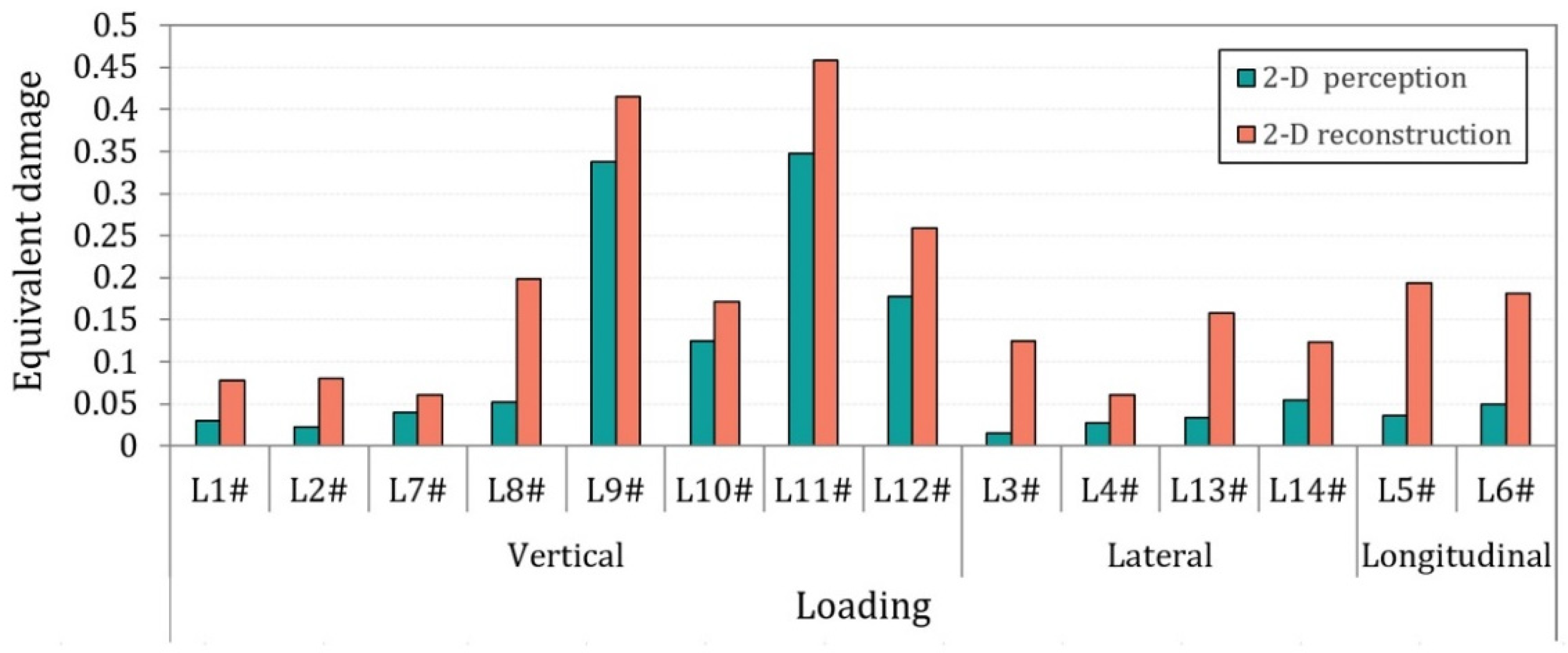
A 2-D equivalent damage comparison histogram for each point is plotted in Figure 16, which is based on the full life-cycle cumulative sum of 32-grade damage spectra at the 14 capture and reconstruction points.
As can be seen from Figure 16 that the equivalent damage is less than 1, which meets the design requirements. The reconstructed damages are greater than the captured due to the multi-directional stress action at reconstruction locations, of which, the 2-D reconstructed equivalent damage at L5# is increased by 0.16 compared to the captured, and the least growth at L7# is 0.02. From the different load types, the result shows that the 2-D equivalent damage of L5#, L11# and L13#, which is mainly subjected to longitudinal load, vertical load and lateral load, reaches 0.19, 0.46 and 0.15, respectively. As above, the maximum equivalent damage is situated at weld joints in near-vertical load cases, followed by longitudinal load cases, and the last is transverse load cases. More attention should be paid to the weak positions of the vertical load’s action, but the loading of lateral forces should not be neglected [30]; a large increase in lateral loads after the reconstruction can also be indicated from the results.
The fatigue damage of the frame is evaluated above based on the operational data on the day of the dynamic stress maximum. To consider the combined effect of the stress maximum and the operational mileage, the daily variation in the fatigue damage value for the 14 measurement points can be counted during the operation period, as shown in Figure 17. The maximum damage that occurred on 2 September appeared in L11# with a value of 1.07 × 10⁻⁵. The damage on 29 September, where the dynamic stress maximum value appeared, is lower, which is due to the different daily operating mileage, so the accumulated damage value is not directly proportional to the dynamic stress value. To eliminate the influence of the daily operating mileage irregularities, the damage of other dates is equated with the mileage of 29 September, as in Figure 18. During the operation period, the maximum equivalent damage occurred on 29 September, with a damage value of 3.86 × 10⁻⁶ at the front gear box base, and the minimum is on 1 October, with a damage value of 1.03 × 10⁻⁷ at the left shaft neck center, which is consistent with the law of changes in operating mileage and peak stress data.
As a result, the maximum total accumulated damage of the bogie frame during the test is 0.0013, which corresponds to the equivalent damage value of 0.32 for the whole life cycle. Compared to 0.35 for the entire life cycle based on the maximum daily damage evaluation, this difference is due to the daily variation in mileage and dynamic stress in actual operation. All of which can meet the design requirements.

5. Conclusions

This paper proposed a stress reconstruction method based on the load identification and experimental fatigue damage evaluation of bogie frames on railway vehicles. The validation of the presented model is conducted by coupled loading simulation and a static loading experiment. Conclusions are as follows:
(1)
A structural stress reconstruction model is derived for the metro bogie frame. The locations of the maximum stress under different load cases are obtained, and reasonable positions are selected to arrange the measurement points with assistance from the FEA. Furthermore, the stress distribution of the frame is reconstructed using the calculated transfer relationship between capture points and large stress points. The results reveal that the stresses after reconstruction are generally larger than those before.
(2)
In light of the relationship between external load and stress in the FE simulation, a load identification model is presented, and the theoretical model is verified by FE simulation under a random load, wherein the maximum deviation does not exceed 1.1 kN, and the minimum deviation is 0 kN. The validation results indicate that there is good agreement between the theoretical model and the numerical simulation.
(3)
Time-history data of the motor car bogie frame was obtained through a vehicle test, and the results show that the stress extreme value after reconstruction is greater than the capture. The maximum equivalent damage of reconstructed and captured is 0.46 and 0.35, respectively. The equivalent damage at different load directions is in descending order of vertical load, longitudinal load and lateral load. Hence, much focus should be on the role of vertical loads and the joint action locations of multiple loads.
(4)
Equivalent damage is evaluated over two assessment methods in the full life cycle, one using maximum daily dynamic stress damage and another using maximum cumulative damage during the whole test period. Both damage assessment methods are satisfied with the design life of the bogie frame, revealing that the current operating condition does not lead to fatigue damage to the frame.

6. Patents

Method and system for stress reconstruction and damage assessment for multi-point surface stress monitoring (ZL202110021975.2).

Author Contributions

Conceptualization, W.Z.; methodology, W.Z. and H.X.; validation, G.Z. and H.X.; investigation, H.W. and C.P.; resources, X.L. (Xifeng Liang) and X.L. (Xiang Liu); writing—original draft preparation, G.Z.; writing—review and editing, H.X. and W.Z.; funding acquisition, H.W. and C.P.; All authors have read and agreed to the published version of the manuscript.

Funding

This research was funded by the National Key R&D Program of China, grant number 2020YFE0204900, the National Science Foundation of Hunan Province, China, grant number 2020JJ4118, the Innovative Province Construction Special of Hunan, China, grant number 2021GK4032, and the Research Innovation Program for Graduate Students of Central South University, China, grant number 1053320192218.

Institutional Review Board Statement

Not applicable.

Informed Consent Statement

Not applicable.

Data Availability Statement

Exclude this statement.

Conflicts of Interest

The authors declare no conflict of interest.

References

  1. Żak, J.; Kurek, D. Multiple Criteria Evaluation of Trams Based on Customers’ Specifications (Expectations) in Selected Countries. Transp. Res. Procedia 2020, 47, 696–703. [Google Scholar] [CrossRef]
  2. Jing, L.; Liu, K.; Ren, M. The Transient Response of Car Body and Side Windows for High-Speed Trains Passing by Each Other in a Tunnel. Compos. Part B Eng. 2019, 166, 284–297. [Google Scholar] [CrossRef]
  3. Cubillo, A.; Vermeulen, J.; Rodriguez de la Peña, M.; Collantes Casanova, I.; Perinpanayagam, S. Physics-Based Integrated Vehicle Health Management System for Predicting the Remaining Useful Life of an Aircraft Planetary Gear Transmission. Int. J. Struct. Integr. 2017, 8, 484–495. [Google Scholar] [CrossRef]
  4. Wang, G.; Wu, C.; Li, S. Effect of Vibration from Highway Vehicle Load on Adjacent Buildings and Its Assessment. IOP Conf. Ser. Earth Environ. Sci. 2019, 267, 052048. [Google Scholar] [CrossRef] [Green Version]
  5. Ferreiro, S.; Arnaiz, A.; Sierra, B.; Irigoien, I. Application of Bayesian Networks in Prognostics for a New Integrated Vehicle Health Management Concept. Expert Syst. Appl. 2012, 39, 6402–6418. [Google Scholar] [CrossRef]
  6. Deng, S.J.; Luan, J.Y.; Tang, L.W.; Wang, W. Research of Vehicle Health Management System Framework Design Based on Teds Sensor. In Proceedings of the 2012 International Conference on Quality, Reliability, Risk, Maintenance, and Safety Engineering, Chengdu, China, 15–18 June 2012; pp. 772–775. [Google Scholar] [CrossRef]
  7. Mizrak, C.; Esen, İ. The Optimisation of Rail Vehicle Bogie Parameters with the Fuzzy Logic Method in Order to Improve Passenger Comfort during Passage over Bridges. Int. J. Heavy Veh. Syst. 2017, 24, 113–139. [Google Scholar] [CrossRef]
  8. Jin, M.; Kosova, G.; Cenedese, M.; Chen, W.; Singh, A.; Jana, D.; Brake, M.R.W.; Schwingshackl, C.W.; Nagarajaiah, S.; Moore, K.J.; et al. Measurement and Identification of the Nonlinear Dynamics of a Jointed Structure Using Full-Field Data: Part II-Nonlinear System Identification. Mech. Syst. Signal Process. 2022, 166, 108402. [Google Scholar] [CrossRef]
  9. Deng, L.; Zou, S.; Wang, W.; Kong, X. Fatigue Performance Evaluation for Composite Osd Using Uhpc under Dynamic Vehicle Loading. Eng. Struct. 2021, 232, 111831. [Google Scholar] [CrossRef]
  10. Xiu, R.; Spiryagin, M.; Wu, Q.; Yang, S.; Liu, Y. Fatigue Life Assessment Methods for Railway Vehicle Bogie Frames. Eng. Fail. Anal. 2020, 116, 104725. [Google Scholar] [CrossRef]
  11. Wang, H.; Liu, W.; Shang, Y. Fatigue Strength Analysis of Domestic Y25 Bogie Welded Frame Based on Hot Spot Stress. China Railw. Sci. 2013, 34, 66–70. [Google Scholar]
  12. Lan, Q.; Song, F. Fatigue Simulation of Railway Car Bogie Frame Based on Multi-Body Dynamics and Finite Element Analysis. J. Phys. Conf. Ser. 2021, 1885, 042057. [Google Scholar] [CrossRef]
  13. Di, J.; Ruan, X.; Zhou, X.; Wang, J.; Peng, X. Fatigue Assessment of Orthotropic Steel Bridge Decks Based on Strain Monitoring Data. Eng. Struct. 2021, 228, 111437. [Google Scholar] [CrossRef]
  14. Liang, Z.; Chai, J.; Na, S.; Ma, T.; Tang, Y. Validity Analysis of Bridge Health Monitoring Data Based on Deep Learning. J. Chongqing Jiaotong Univ. 2021, 40, 78–83. [Google Scholar]
  15. Wang, C.; Meng, G.; Yuan, L.; Liu, J. Numerical Simulation Analysis of Fatigue Life of a New High Speed Bus Frame. China Railw. Sci. 2001, 03, 94–98. [Google Scholar]
  16. Yaohui, L. Study on Fatigue Reliability of Welded Frame of Railway Passenger Car Bogie. Ph.D. Thesis, Southwest Jiaotong University, Chengdu, China, 2011. [Google Scholar]
  17. Bingrong, M. Fatigue Simulation of Locomotive Body Structure Based on Multi-Body Dynamics and Finite Element Method. Ph.D. Thesis, Southwest Jiaotong University, Chengdu, China, 2007. [Google Scholar]
  18. Zeng, L.; Zhao, J.; Meng, Y. Vibrational Fatigue Failure Prediction of a Brake Caliper Used for Railway Vehicles Based on Frequency Domain Method. J. Phys. Conf. Ser. 2021, 1948, 012091. [Google Scholar] [CrossRef]
  19. Zhou, X.; Zhang, X. Thoughts on the Development of Bridge Technology in China. Engineering 2019, 5, 1120–1130. [Google Scholar] [CrossRef]
  20. Spiroiu, M.A. Reliability Model of Freight Bogie Damper Based on Real Field Data. IOP Conf. Ser. Mater. Sci. Eng. 2021, 1037, 012056. [Google Scholar] [CrossRef]
  21. Zhang, C.; Fu, Y.; Li, Y.; Li, J. Distributed Dynamic Load Identification of Aircraft Skin Based on Strain Modal Method. Equip. Environ. Eng. 2020, 17, 113–117. [Google Scholar] [CrossRef] [Green Version]
  22. Coules, H.E.; Smith, D.J.; Abburi Venkata, K.; Truman, C.E. A Method for Reconstruction of Residual Stress Fields from Measurements Made in an Incompatible Region. Int. J. Solids Struct. 2014, 51, 1980–1990. [Google Scholar] [CrossRef] [Green Version]
  23. Lampone, L.W. A Positive Polynomial Expansion Problem in Minimum Variance Smoothing. SIAM J. Math. Anal. 1978, 9, 500–514. [Google Scholar] [CrossRef]
  24. Nakamura, T. Local Stress-Field Reconstruction around Holes in a Plate Using Strain Monitoring Data and Stress Function. J. Appl. Mech. 2018, 86, 031005. [Google Scholar] [CrossRef]
  25. Wang, B.J.; Li, Q.; Ren, Z.S.; Sun, S.G. Improving the Fatigue Reliability of Metro Vehicle Bogie Frame Based on Load Spectrum. Int. J. Fatigue 2020, 132, 105389. [Google Scholar] [CrossRef]
  26. Tae, K.H. Fatigue Prediction of Spot Welded Joints Using Equivalent Structural Stress. Mater. Des. 2005, 28, 837–843. [Google Scholar]
  27. HG/T 20580-2011; Specification of Design Base for Steel Chemical Vessels. China Standard Press: Beijing, China, 2011; p. 41.
  28. TB/T 2368-2005; Test Method for Strength of Power Bogie Frames. China Standard Press: Beijing, China, 2005; p. 18.
  29. Chandrasekhar, S.; Liu, X. Chapter 3-Advances in Tb/S Superchannels. In Optical Fiber Telecommunications, 6th ed.; Kaminow, I.P., Li, T., Willner, A.E., Eds.; Academic Press: Boston, MA, USA, 2013; pp. 83–119. [Google Scholar]
  30. Xie, X.Y.; Jin, G.L.; Wang, R.L. Evaluation of Bogie Frame Safety of Shanghai Metro Line 1 by 3d Fem Analysis. AIP Conf. Proc. 2010, 1233, 1140. [Google Scholar]
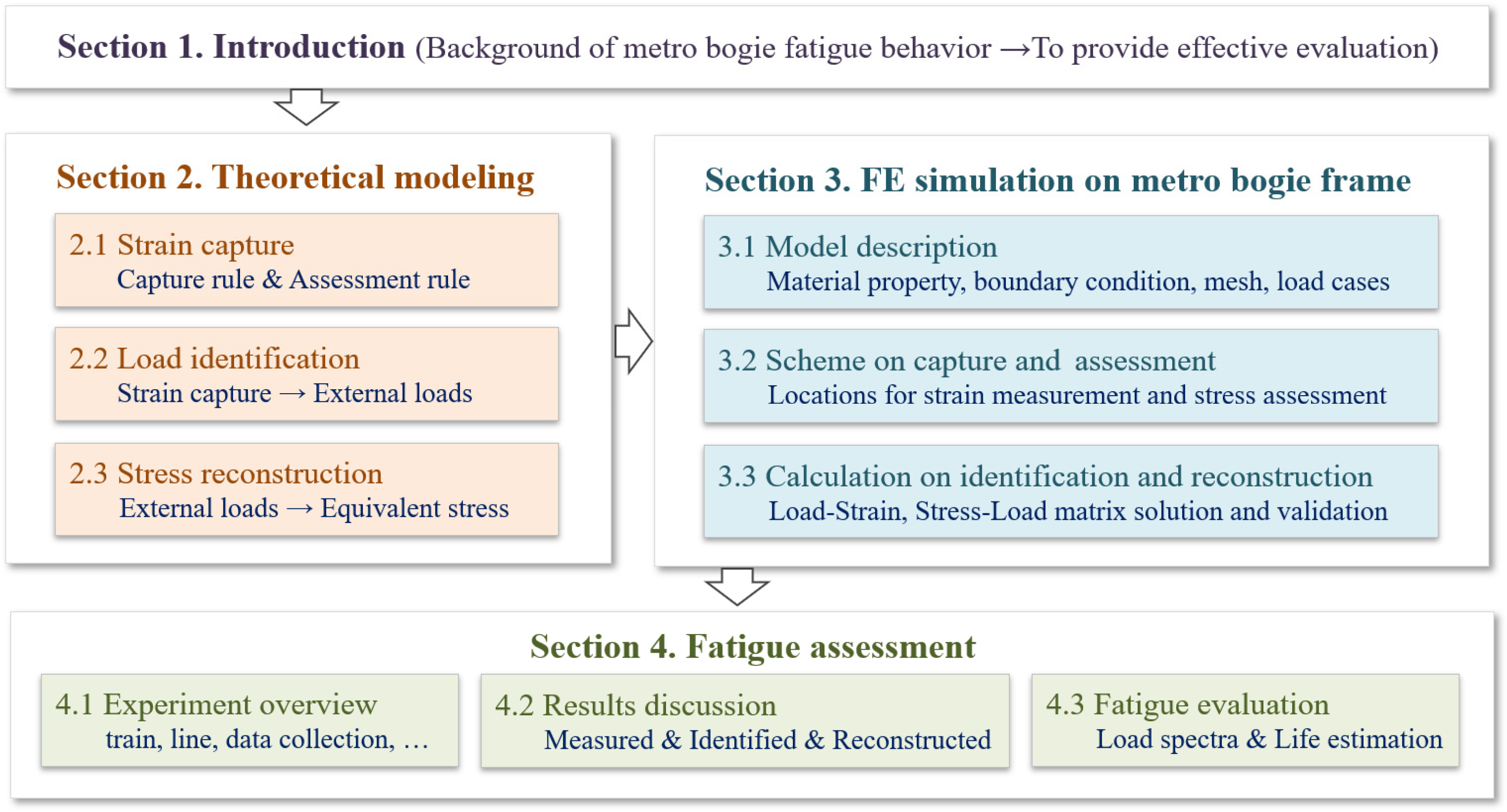
Figure 1. The framework of this paper.
Machines 10 01003 g001
Figure 2. 3D model and boundary conditions.
Machines 10 01003 g002
Figure 3. Load coupling reference point.
Machines 10 01003 g003
Figure 4. Location of capture and assessment points.
Machines 10 01003 g004
Figure 5. Contour bar plot of captured strain and reconstructed stress to identified loads. (a) Surface strain-identified load; (b) Reconstructed stress-identified load.
Machines 10 01003 g005
Figure 6. Contour bar plot of the validation result. (a) Difference between the identified and given loads; (b) surface strain.
Machines 10 01003 g006
Figure 7. (a) Beijing metro line and (b) its passenger flow.
Machines 10 01003 g007
Figure 8. Test bogie location in the 6-car metro train (T: trailer car; M: motor car).
Machines 10 01003 g008
Figure 9. Strain gauge bonding at capture locations on the bogie frame. (a) Right air spring base welds; (b) Left air spring base welds; (c) Left longi-cross beam joint welds; (d) Right longi-cross beam joint welds; (e) Front traction rod base welds; (f) Rear traction rod base welds; (g) Front motor base welds; (h) Rear motor base welds; (i) Left side-cross beam joint welds; (j) Right side-cross beam joint welds; (k) Front gear box base welds; (l) Rear gear box base welds; (m) Left lateral damper base welds; (n) Right lateral damper base welds.
Machines 10 01003 g009
Figure 10. Daily mileage history in test period.
Machines 10 01003 g010
Figure 11. Peak stress detection during test period.
Machines 10 01003 g011
Figure 12. Time-history curves. (a) Measured stress; (b) identified load; (c) reconstructed stress.
Machines 10 01003 g012
Figure 13. Bar plot of peak stress between measured and reconstructed values. NOTE: L1# represents the collective name of L1#SURF and L1#STRU, the same as in other points.
Machines 10 01003 g013
Figure 14. Load spectrum classification of 8 loading position types.
Machines 10 01003 g014
Figure 15. Measured cycles and damage graphs of capture and reconstruction stress. (a) Air spring base (L1#); (b) lateral stop base(L3#); (c) traction rod base(L6#); (d) motor base(L7#); (e) braking base(L9#); (f) shaft neck center(L10#); (g) gear box base(L11#); (h) lateral damper base(L14#).
Machines 10 01003 g015aMachines 10 01003 g015b
Figure 16. Maximum 2-D equivalent damage comparison of capture and reconstruction.
Machines 10 01003 g016
Figure 17. Fatigue damage during the test period.
Machines 10 01003 g017
Figure 18. Equivalent damage during the test period.
Machines 10 01003 g018
Table 1. Mechanical parameters of bogie frame structures.
ComponentMaterialElastic Modulus
E (GPa)
Poisson’s Ratio υDensity
ρ (g cm−3)
Yield Stress
σys (MPa)
Fatigue Limit
σlim (MPa)
Steel plateQ3452060.37.85345110
Cross beamSMA490BW2060.37.85355110
Table 2. Mechanical parameters of welding electrodes.
MaterialTensile Strength
(MPa)
Yield Strength
(MPa)
Elongation (%)
J50749040020
Table 3. Load case summary.
Load CaseLoad [28] (Ministry of Railways 2005) Fi(max) 
(kN)
Load PositionLoad Type and Direction
LC1#−100Right air spring baseVertical load (-Z)
LC2#−100Left air spring baseVertical load (-Z)
LC3#−68.67Right lateral stop baseLateral load (-Y)
LC4#68.67Left lateral stop baseLateral load (Y)
LC5#82.4Front traction rod baseLongitudinal load (X)
LC6#82.4Rear traction rod baseLongitudinal load (X)
LC7#−28.5Front motor baseVertical load (-Z)
LC8#−28.5Rear motor baseVertical load (-Z)
LC9#10Left braking baseTorsional load (Z)
LC10#10Left shaft neck centerTorsional load (Z)
LC11#−50Front gear box baseVertical load (-Z)
LC12#50Rear gear box baseVertical load (Z)
LC13#3Left lateral damper baseLateral load (Y)
LC14#3Right lateral damper baseLateral load (Y)
Table 4. Capture and assessment locations.
Location LabelsLocation Descriptions
L1#(SURF), L1#(STRU) || L2#(SURF), L2#(STRU)Left || Right air spring base welds
L3#(SURF), L3#(STRU) || L4#(SURF), L4#(STRU)Left || Right lateral stop base welds
L5#(SURF), L5#(STRU) || L6#(SURF), L6#(STRU)Front || Rear traction rod base welds
L7#(SURF), L7#(STRU) || L8#(SURF), L8#(STRU)Front || Rear motor base welds
L9#(SURF) || L10#(SURF), L10#(STRU)Left || Right side-cross beam joint welds
L9#(STRU)Left brake base welds
L11#(SURF), L11#(STRU) || L12#(SURF), L12#(STRU)Front || Rear gear box base welds
L13#(SURF), L13#(STRU) || L14#(SURF), L14#(STRU)Left || Right lateral damper base welds
Note: LN#(SURF) denotes the capture locations, and LN#(STRU) denotes the assessment locations.
Table 5. Comparison between identified and given loads (kN).
Random
Load Case
Load Types
F1F2F3F4F5F6F7F8F9F10F11F12F13F14
RLC1#GV−20.630.7 −65.744.8 45.4 53.3 15.6 24.3 9.9 5.8 −36.719.7 0.5 0.5
ID−19.631.4 −65.145.345.8 53.9 16.0 24.6 10.5 5.8 −36.619.8 0.8 0.7
RLC2#GV93.0 92.9 −8.6 −9.7 21.6 50.6 −12.8 6.3 7.6 −7.4 10.8 −27.8 0.3 −1.3
ID93.8 93.8 −7.6 −9.1 21.7 51.2 −11.8 7.0 7.9 −6.7 11.6 −27.3 1.2 −0.3
RLC3#GV11.3 −95.7 −14.1 −10.1 −57.3 −8.5 2.9 −28.1 −8.0 −5.2 0.8 0.0 2.1 2.0
ID11.4 −95.2 −13.5 −9.7 −57.2 −8.2 3.7 −27.9 −7.8 −4.6 1.7 0.3 2.3 2.9
RLC4#GV43.6 92.6 −64.8 −23.9 45.8 57.6 0.5 13.5 −1.5 −3.3 20.9 49.7 2.6 −1.9
ID43.8 93.6 −64.6 −22.9 46.0 58.1 1.3 14.1 −1.5 −2.4 21.7 50.6 3.2 −1.7
RLC5#GV75.9 −35.1 57.1 −22.3 −72.2 27.1 −18.6 −8.0 −0.6 3.7 −11.1 −4.9 −0.3 2.5
ID76.1 −34.7 57.3 −21.9 −72.0 27.7 −17.7 −7.4 −0.4 4.0 −10.9 −4.7 0.5 2.7
RLC6#GV−99.3 −70.0 −19.7 −43.3 31.8 −49.5 18.3 −9.6 −5.5 −1.4 −11.1 −27.2 −1.0 −0.8
ID−98.8 −69.1 −18.6 −43.2 32.2 −49.3 18.8 −8.6 −5.3 −0.9 −10.5 −26.1 0.0 −0.3
RLC7#GV−23.0 82.1 −9.8 44.5 71.9 11.0 10.0 0.9 6.4 3.3 −14.0 5.0 2.3 1.6
ID−22.4 82.7 −9.6 45.2 71.9 11.8 10.4 1.3 7.4 3.6 −13.0 6.1 2.6 1.7
RLC8#GV60.9 90.9 −39.6 −39.9 52.3 −47.4 −6.0 15.5 −1.4 9.9 −5.5 40.0 2.8 2.8
ID61.1 90.9 −39.1 −39.5 52.7 −47.0 −5.2 16.0 −0.5 10.5 −5.2 40.3 3.8 2.9
RLC9#GV77.5 93.5 48.6 39.1 0.8 67.1 4.5 −4.6 −6.4 −8.8 −48.9 47.2 1.5 1.8
ID78.1 93.6 48.8 39.7 1.3 67.5 5.2 −3.6 −5.8 −8.1 −48.2 48.1 2.4 2.2
RLC10#GV−69.3 −18.2 −67.4 −37.0 30.9 37.3 −3.7 −7.7 8.6 4.1 19.9 −7.0 0.2 −0.2
ID−69.3 −17.8 −66.3 −36.9 31.7 37.4 −3.4 −7.2 9.2 4.9 20.9 −6.7 1.0 0.0
Table 6. Fatigue parameters of bogie frame material.
StructureS-N Curve ParameterLimit Cycles (×104)Design Mileage (km)Running Mileage (km)
mc
Base metal54.484 × 10171000396 × 10416,854
Welding joints3.52.7919 × 1013200
Publisher’s Note: MDPI stays neutral with regard to jurisdictional claims in published maps and institutional affiliations.