Muscle Selection Using ICA Clustering and Phase Variable Method for Transfemoral Amputees Estimation of Lower Limb Joint Angles

Abstract

Surface electromyography(sEMG) signals are used extensively in the study of lower limb locomotion, capturing and extracting information from various lower limb muscles as input for powered prostheses. Many transfemoral amputees have their lower limbs completely removed below the knee due to disease, accident or trauma. The patients only have the muscles of the thigh and cannot use the muscles of the lower leg as a signal source for sEMG. In addition, wearing sEMG sensors can cause discomfort to the wearer. Therefore, the number of sensors needs to be minimized while ensuring recognition accuracy. In this paper, we propose a novel framework to select the position of sensors and predict joint angles according to the sEMG signals from thigh muscles. Specifically, a method using ICA clustering is proposed to statistically analyze the similarity between muscles. Additionally, a mapping relationship between sEMG and lower limb joint angles is established by combining the BP network and phase variable method, compared with the mapping using only neural networks. The results show that the proposed method has higher estimation accuracy in most of the combinations. The best muscle combination is vastus lateralis (VL) + biceps femoris (BF) + gracilis (GC) (${\gamma }_{knee}$ = 0.989, ${\gamma }_{ankle}$ = 0.985). The proposed method will be applied to lower limb-powered prostheses for continuous bioelectric control.

1. Introduction

The results of the sixth census in China show that the population of disabled people with lower limb disability due to work-related injuries, natural disasters and traffic accidents has reached 1.58 million, and it is accompanied by an increasing trend year by year [1]. Lower limb amputation not only affects the normal life of people with disabilities but also leads to further physical damage due to improper movement. Currently, most of the major commercial prostheses on the market are passive prostheses, which do not provide energy and require the wearer to use the residual lower limb and hip strength to maintain movement, which consumes more energy. However, active prostheses can provide enough power to help patients move like people without disabilities. Researchers have used various mechanical sensors to develop powered prostheses, such as Inertial Measurement Units (IMU) and plantar force sensors [2]. Moreover, sEMG signals have become an important information input for predicting lower limb motion due to their non-invasive nature and rich information. Tahir Hussain et al. use different classifiers to identify gait patterns by acquiring sEMG signals from 11 muscles of the lower limb [3]. Wang et al. use sEMG signals from five muscles of the lower limb to map sEMG signals to knee angles using Elman networks for estimating lower limb motion angles [4].

Due to the interaction between external noise and muscles, the sEMG signals on each muscle are generated by the superposition of multiple sources [5], which can be filtered out by a filtering method for the noise of different frequencies. For signals mixed with other muscles, multiple internal sources need to be separated based on the sEMG signals. In addition, the number and location of sEMG sensors greatly affect the prosthetic control performance. There are some methods using high-density sensors to improve the accuracy of recognition [6], but the use of multiple channels may be uncomfortable for the amputees, increase the computational cost and affect the real-time control. Therefore, it is necessary to select the appropriate number and location of thigh muscles among the many. Several studies have been conducted recently to address the above problem. A. Dogukan Keles et al. collected sEMG signals from five muscles of the lower limb (tibialis anterior (TA), medial gastrocnemius (MG), rectus femoris (RF), biceps femoris (BF) and gluteus maximus (GM)) as inputs. They used Pearson correlation coefficients and root mean square error to rank the muscle combination changes and select the location of sensor placement [7]. However, this approach is suitable only when the number of sensors is small. I. S. Dhindsa et al. obtained sEMG signals from 18 muscles. Principal component analysis was then conducted on the predicted force variable. Additionally, they obtained the most suitable muscles for controlling the exoskeletal knee joint four-channel system and five-channel system, respectively [8]. However, the method of principal component analysis can only ensure orthogonality between components [9], which will lose a lot of information and lead to inaccurate estimation.

Establishing the mapping relationship between lower limb thigh muscles and knee and ankle joint angles not only allows the selection of a suitable thigh muscle as a signal source based on the accuracy of angle prediction but also, this motion estimation plays an important role in the motion estimation of lower limb prostheses. Currently, there are two main methods for the continuous estimation of joint angles, and the first method uses a biomechanical model for joint angle estimation. For example, Han et al. proposed a myoelectric state space model to predict joint angles [10], which is based on the Hill muscle model and forward dynamics. However, the physiological properties of muscles undergo complex changes during actual exercise, and there are many physiological parameters that cannot be directly measured. The second approach is to use regression models to predict joint angles. For example, Cheron. G et al. collected sEMG signals of six lower limb muscles and constructed a dynamic recurrent neural network (DRNN) prediction model to estimate lower limb joint angles [11]. Chen et al. recorded information on 10 muscles associated with lower limb movements and used a BP neural network to map the best sEMG features to finite element joint angles [12]. In the above research, sEMG signals were extracted from the thigh and calf muscles, and their best results were 0.97 and 0.95 (Pearson correlation coefficient ($\gamma$)), respectively, for the knee and ankle [12]. However, for transfemoral amputees, sEMG signals from calf muscles are unavailable. Because the motions of the knee and ankle are highly related to calf muscles, using only thigh muscle information to predict knee and ankle angles will lead to inaccuracy.

This paper proposes a novel framework to select the location of muscles and predict joint angles according to the sEMG signals from thigh muscles. Based on the framework, we first use the Icasso method [13,14,15,16] to choose the most appropriate position, the number of thigh muscles and to preprocess our signals as inputs. Then, deep belief network (DBN) features are extracted after the input data are sent to the DBN network. DBN features, together with input data, are sent to the BP network to obtain the thigh angle, while thigh angular velocity can be obtained by the differentiator. Finally, the phase variable is obtained from the thigh motion, and the knee and ankle angles can be calculated by the phase variable method. In this paper, using only the thigh muscles, we reached ${\gamma }_{knee}$ = 0.989, ${\gamma }_{ankle}$ = 0.985.

This paper is divided into four parts, and the details of each part are as follows: the first part introduces the current method of selecting sensors and establishes the mapping relationship between thigh muscle and knee and ankle joints. Additionally, this part also summarizes the work objective of this paper. The second part describes our proposed novel framework. Specifically, the acquisition of data, the processing of the signal and mapping to the knee and ankle joint angles are shown. The third part provides the experimental results and our discussion. The fourth part summarizes the whole paper.

2. Materials and Methods

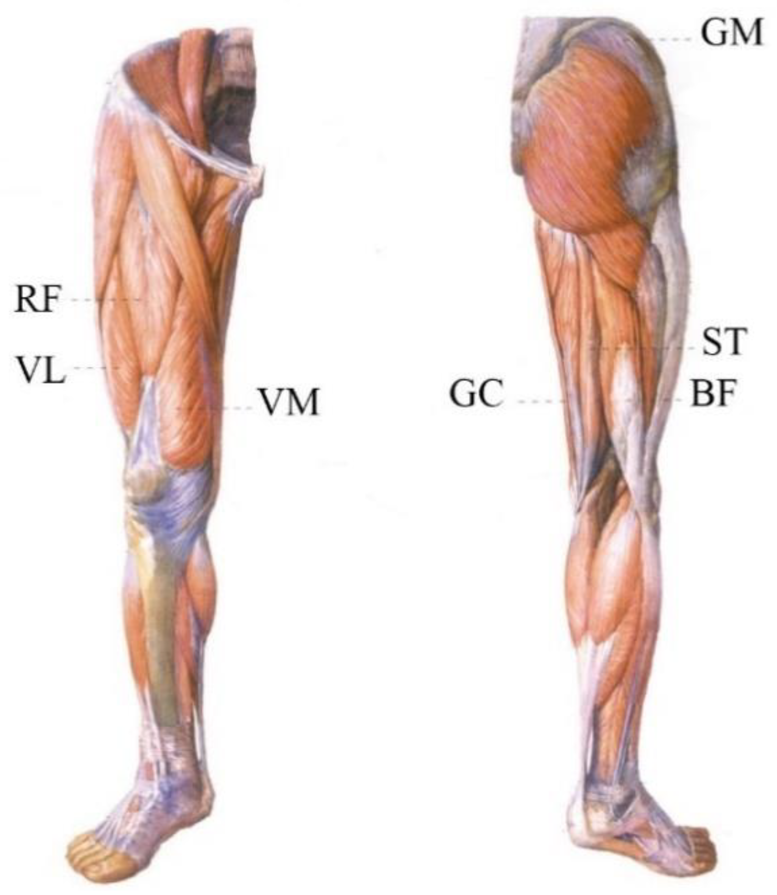
2.1. Source of Data

The sEMG and lower limb motion data used in this paper were obtained from the database created by Jonathan Camargo et al. [17]. The database contains human motor gait data from different individuals. In this paper, we selected the locomotor gait data of 12 healthy subjects aged 20–33 years on a treadmill with a speed of 0.5–1.85 m/s and an incline of 0. The subjects’ body-specific information is shown in

Table 1. Information on the subjects.

Subject ID	Age	Gender	Height (m)	Mass (kg)	Subject ID	Age	Gender	Height (m)	Mass (kg)
AB09	21	F	1.63	63.5	AB18	19	F	1.82	60.1
AB10	22	M	1.75	83.9	AB23	20	M	1.80	76.8
AB11	21	M	1.75	77.1	AB24	21	F	1.73	72.6
AB12	24	M	1.74	86.2	AB25	20	F	1.63	52.2
AB14	22	F	1.52	58.4	AB28	33	F	1.69	62.1
AB15	21	M	1.78	96.2	AB30	31	M	1.77	77.0

, and the subjects included six men and six women. Because our research focuses on transfemoral amputees, we selected seven muscles on the thigh as signal sources for all subjects, namely vastus medialis (VM), vastus lateralis (VL), rectus femoris (RF), biceps femoris (BF), semitendinosus (ST), and gracilis (GC) and gluteus medius (GM), the specific locations of which are shown in Figure 1. The sEMG signals were sampled at 1000 Hz and digitally adjusted using a band-pass filter (cut-off frequency of 20 Hz–400 Hz, Butterworth order of 20). The sEMG signals were then processed to establish the mapping relationship with the knee and ankle joints and to select the appropriate muscle acquisition point, as shown in Figure 2.

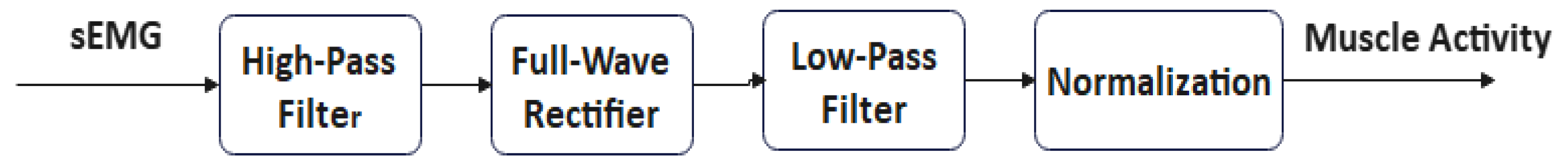
2.2. Signal Preprocessing

Raw sEMG signals are weak and easily influenced by noise, such as internal power lines and nature, so the raw sEMG signals must undergo a series of processing before analysis. The usual processing steps are shown in Figure 3. However, due to differences in skin condition, electrode position and the experimenter, the signals are normalized by Equation (1).

$$x_{new}=\frac{x-x_{\min }}{x_{\max }-x_{\min }},$$

(1)

where $x$ is the data before normalization, and $x_{\max }$ and $x_{\min }$ denote the maximum and minimum values of the data, respectively. $x_{new}$ are the normalized data, which referred to as muscle activity. The processed muscle activity is distributed between 0 and 1. After normalization, the signals will be smoother, and the features will be better extracted.

2.3. ICA Clustering Method

Because of the different initial values of the independent component analysis and the fact that the calculation is based on the minimization or maximization of the objective function, the independent components are estimated differently each time. It is necessary to use the interlayer clustering method to select the appropriate classes. At the same time, the Icasso method is widely used for biomedical signal processing, such as finding signal data sources for non-targeted metabolomics studies [13], extracting mental fatigue features [14] and extracting independent spatial maps and their corresponding time courses from fMRI data [16]. In this paper, we used the Icasso method to select the best location for acquiring sEMG signals. Icasso is a combination method of ICA and clustering, which is computed by executing ICA and clustering procedures multiple times. The specific content is as follows.

2.3.1. Independent Component Analysis of sEMG

In the ICA analysis of sEMG data, the basic model of ICA is $X=AS$, where $X$ is the mixed signal detected by the sensors and $X$ is a matrix of $m\times n$, $m$ is the sampling point of each sensor, $n$ is the number of sensors and $X={[x_1,\cdots ,x_m]}^T$. $S={[s_1,\cdots ,s_v]}^T$ is a $v\times n$ source matrix. Each observed random variable $x_m$ is obtained by linearly combining the independent components $s_1,\cdots ,s_v$. Additionally, each $a_{ij}$ in the mixing matrix $A$ is a linear superposition of the mixing coefficients. The purpose of the ICA algorithm is to determine the decomposition matrix $W$, so that $S=WX$ can be used to estimate the sources under the assumption of statistical independence of the sources.

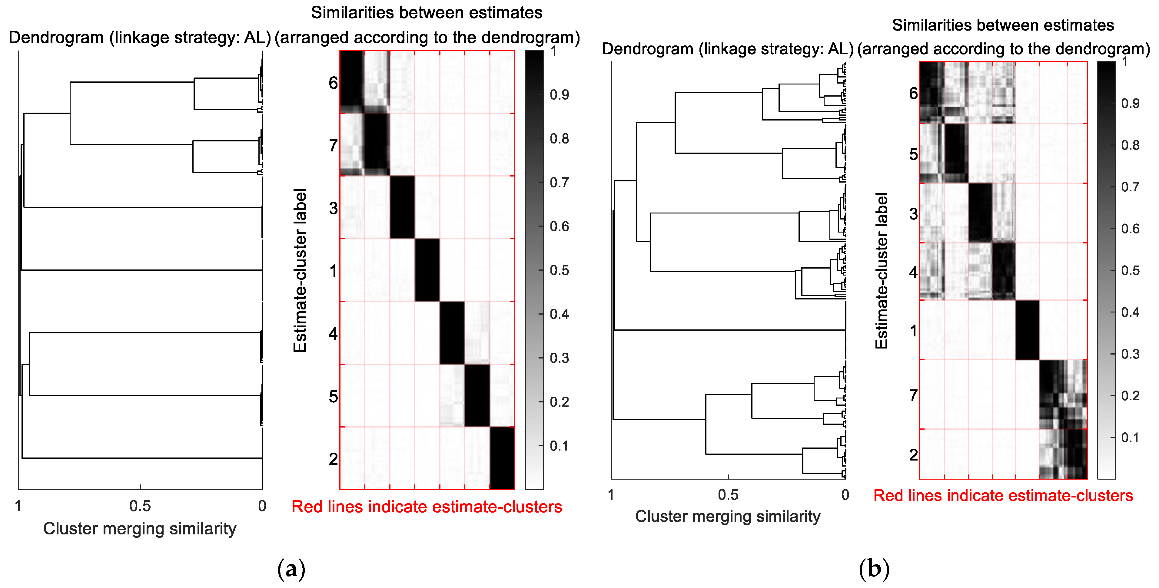
2.3.2. Interlayer Clustering

Since the ICA algorithm is stochastic in nature, the results of every algorithm run may be different. The independent components obtained by one ICA algorithm may not be accurate, so the independent components need to be obtained by the statistical results of multiple operations. Each estimated independent component is a point in space, so the points are gathered by the method of interlayer clustering with Equation (2) and mutual similarity criterion [18]. The partitioning of the clusters is obtained visually in the form of a tree diagram.

$${\sigma }_{ij}=\left|r_{ij}\right|,$$

(2)

where $r_{ij}$ is the intercorrelation relationship. ${\sigma }_{ij}$ is the similarity matrix, representing the similarity between the estimated independent variables.

Reliable, independent component estimates form a cluster in space. As shown in the following equation, we use indicators $I_q$ to react to the calculation of the quality of the cluster [18].

$$I_q\left(C_m\right)=\frac{1}{{\left|C_m\right|}^2}{\displaystyle \sum _{i,j\in C_m}{\sigma }_{ij}}-\frac{1}{\left|C_m\parallel C_{-m}\right|}{\displaystyle \sum _{i\in C_m}{\displaystyle \sum _{j\in C_{-m}}{\sigma }_{ij}}},$$

(3)

where $C_m$ represents the indicator cluster belonging to the m cluster, and $C_{-m}$ represents the indicator cluster that does not belong to the m cluster. $I_q$ is calculated by the difference between the average intra-cluster similarity and the average inter-cluster similarity. The ideal cluster has a $I_q$ value of 1. When the compactness within the cluster becomes weaker, the $I_q$ value becomes smaller. Therefore, the closer the 1 value is to $I_q$, the more concentrated the estimated independent components are and the higher the quality of the cluster. Then, the independent components from the Icasso method are used as inputs to the regression network, corresponding to the knee and ankle angles in lower limb motion.

2.4. Feature Extraction and Dimensionality Reduction

In regression methods, the extraction and selection of features have an important impact on the learning efficiency and estimation accuracy of regression networks [12]. In previous work, the method of principal component analysis was often used to extract the features. However, the method of PCA is a linear dimensionality reduction method with limited ability to extract nonlinear components from sEMG signals, so in order to automatically learn complex structural components from sEMG signals and perform dimensionality reduction, this paper uses the DBN method proposed by Hinton [19], which uses a multilayer network. The independent components of the input are reconstructed to extract the nonlinear partial components of the data.

2.5. Mapping of Neural Networks and Phase Variable Methods

Establishing the mapping relationship between the extracted features and the knee and ankle joint angles is also a focus. Because there are nonlinear features in sEMG signals, a neural network with a strong nonlinear mapping ability is required to establish the relationship between the features and the joint angles. Estimating the knee and ankle joints from the sEMG signals of the thigh will lead to low accuracy [7], but it will be much more accurate to estimate the thigh angles. For human lower limb motion, the thigh motion angle can represent the periodic motion continuously alone [20]. Therefore, in this paper, the thigh angle was obtained from the BP network using the nonlinear features, and the thigh angle output was calculated using the following equation.

$$\mathsf{\theta }=W_{\mathrm{out} }\left[\frac{2}{1+e^{-2\left(W_{\mathrm{in}}y+b_{\mathrm{in}}\right)}}-1\right]+b_{\mathrm{out}},$$

(4)

where $W_{\mathrm{in} }$ and $W_{\mathrm{out} }$ are the input weights and output weights of a particular layer. $b_{\mathrm{in}}$ and $b_{\mathrm{out}}$ are the corresponding threshold vectors. The gait phase variables are constructed from the estimated thigh angles, which are computed in the phase variable estimation in Figure 1. To describe gait kinematics by thigh angles, a basic gait kinematic model is required. A common method is to use a finite basis function weighted summation [21]. Since the Fourier series can represent any periodic signal, the basis function can be chosen as a finite Fourier series [22], as shown in the following equation.

$$q(\phi )=a_0+{\displaystyle \sum _{i=1}^F\left[a_i\cos (i\omega \phi )+b_i\sin (i\omega \phi )\right]},$$

(5)

where $a_0$, $a_i$ and $b_i$ represent the Fourier series, which is calculated based on the average human data. $F$ is the order, $\omega$ is the frequency of the thigh angle trajectory, $\phi$ is the gait phase variable and $q$ is the knee and ankle joint angle. The phase variable method is used to obtain the knee and ankle joint angles, thus indirectly establishing the mapping between sEMG signals and the knee and ankle joints of the lower limbs.

2.6. Evaluation of the Angle Estimation

To evaluate the predictive effect on knee and ankle joints, the Root Mean Square Error (RMSE) and Pearson correlation coefficient (γ) of predicted and measured angles are evaluated as metrics in this paper. A threshold of 0.95 was chosen to indicate successful correlation [12] and to select the appropriate combination of muscles.

3. Results

The experimental data of the subjects were extracted from the database at speeds of 0.65, 1.35, 1.7 and 1.0 m/s on the treadmill with an incline of 0. The seven-channel sEMGs of the knee and ankle joints of the 12 subjects were obtained separately for each speed duration of 30 s, of which 80% was used as the training set, and 20% was used as the test set. The seven dimensions of raw sEMG data were analyzed by independent components analysis. Then, independent components were applied to Icasso for clustering. Figure 4 shows the dendrograms of independent component clustering for two subjects, AB14 and AB30.

As can be seen from Figure 4, the left panel shows that the points can become a cluster when moving left in the dendrogram. The right panel shows that the estimated independent components are divided into clusters, and the grayscale in the graph represents interrelationships between each independent component. Icasso divided the independent components of subjects AB14 into three clusters, (3, 6, 7), (4, 5, 1) and (1). The estimated independent components of the subjects AB30 were also divided into three clusters, (2, 3, 5, 4), (6, 7) and (1).

Because the ICA algorithm is random, the result of each calculation may be different in each run. Additionally, the division of an ordinal number of clusters is the order after cluster quality calculation, which cannot correspond to the position of the sensor. In this paper, we obtained a method in which the estimated values of independent components corresponded to the original signals according to the decomposition matrix.

Table 2. The clusters divided by Icasso for the 12 subjects and the sensor locations corresponding to the independent components.

Subject ID	Class	Cluster 1	Cluster 2	Cluster 3	Cluster 4
AB09	IC	6, 7, 5	4, 1	3, 2
	Sensors	RF, VL, VM	BF, ST	GC, GM
AB10	IC	6, 7, 5, 4	1	2, 3
	Sensors	VM, VL, RF, GM	GC	BF, ST
AB11	IC	6, 7, 3, 1	5, 4	2
	Sensors	VM, VL, RF, GC	BF, ST	GM
AB12	IC	4, 3	2	1	6, 7, 5
	Sensors	BF, ST	GC	GM	VM, VL, RF
AB14	IC	6, 7, 3, 1	4, 5	2
	Sensors	VM, VL, RF, GM	BF, ST	GC
AB15	IC	6, 7, 5, 3	2, 4	1
	Sensors	VM, VL, RF, GM	BF, ST	GC
AB18	IC	6, 7, 4, 2	1	3, 5
	Sensors	VM, VL, RF, GM	GC	BF, ST
AB23	IC	5, 6, 7	1, 3	2, 4
	Sensors	VM, VL, RF	GC, GM	BF, ST
AB24	IC	6, 7, 4, 5	3	1, 2
	Sensors	VM, VL, RF, GM	GC	ST, BF
AB25	IC	6, 5, 4	1	2, 3	7
	Sensors	RF, VM, VL	GM	ST, BF	GC
AB28	IC	6, 7, 4	3, 5	2	1
	Sensors	VM, VL, RF	ST, BF	GM	GC
AB30	IC	2, 3, 7	1	5, 6	4
	Sensors	VM, VL, RF	GM	BF, ST	GC

The shaded cells show the sensors corresponding to the independent components.

shows the clusters divided by Icasso for the 12 subjects and the sensor locations corresponding to the independent components. For example, in the first experiment of AB12, the independent components were divided into four clusters, (4, 3), (2), (1), (6, 7, 5), and the sensor locations corresponding to the four clusters were (BF, ST), (GC), (GM) and (VM, VL, RF).

From the clustering data of the two experiments of 12 subjects, it can be seen that seven sensor data are clustered into three clusters or four clusters. Three clusters are divided into (VM, VL, RF), (BF, ST) and (GC, GM), and four clusters are divided into (VM, VL, RF), (BF, ST), (GC) and (GM). We can conclude that in the lower limb thigh muscles, VM, VL and RF are more similar, BF and ST are more similar and GC and GM are not very similar and can be divided into one cluster or separated. Therefore, after reducing the number of sensors on the thigh to three or four, we were able to discuss the effects on prediction accuracy separately and select the appropriate combination. We selected the sEMG data of each combination of AB14 of the subjects. Then, the knee and ankle joint angle was calculated according to the process shown in Figure 1. The RMSE and correlation coefficient of knee and ankle angle prediction for each muscle combination are shown in

Table 3. The comparison of three muscle combinations for the subject AB14.

Variation	BP				BP + PHASE
	Knee		Ankle		Knee		Ankle
	RMSE [Deg]	γ (r)	RMSE [Deg]	γ (r)	RMSE [Deg]	γ (r)	RMSE [Deg]	γ (r)
VM + BF + GC (1)	7.071 ± 0.105	0.933	4.605 ± 0.124	0.875	4.817 ± 0.129	0.971	2.896 ± 0.066	0.958
VL + BF + GC (2)	9.926 ± 0.513	0.860	5.624 ± 0.226	0.810	2.813 ± 0.066	0.989	1.794 ± 0.058	0.985
RF + BF + GC (3)	9.173 ± 0.675	0.888	4.995 ± 0.137	0.847	6.129 ± 0.248	0.948	3.304 ± 0.078	0.942
VM + ST + GC (4)	7.171 ± 0.107	0.935	4.501 ± 0.092	0.887	4.421 ± 0.052	0.975	2.722 ± 0.063	0.963
VL + ST + GC (5)	8.257 ± 0.121	0.914	5.641 ± 0.010	0.811	3.738 ± 0.085	0.980	2.278 ± 0.046	0.973
RF + ST + GC (6)	9.231 ± 1.076	0.898	5.054 ± 0.324	0.857	6.981 ± 0.790	0.931	3.645 ± 0.299	0.926
VM + BF + GM (7)	8.056 ± 0.256	0.911	4.711 ± 0.221	0.878	6.300 ± 0.960	0.942	2.483 ± 0.286	0.963
VL + BF + GM (8)	12.864 ± 0.429	0.747	6.464 ± 0.171	0.726	4.553 ± 0.593	0.972	1.736 ± 0.333	0.983
RF + BF + GM (9)	9.156 ± 0.467	0.886	4.975 ± 0.229	0.854	6.541 ± 1.103	0.937	3.531 ± 0.507	0.928
VM + ST + GM (10)	7.440 ± 0.179	0.924	4.252 ± 0.113	0.896	9.115 ± 0.575	0.882	5.051 ± 0.253	0.857
VL + ST + GM (11)	8.730 ± 0.385	0.900	5.468 ± 0.242	0.827	9.819 ± 0.736	0.863	5.277 ± 0.330	0.838
RF + ST + GM (12)	9.238 ± 0.467	0.891	4.747 ± 0.084	0.873	12.033 ± 1.276	0.794	6.679 ± 0.657	0.737

The shaded cells show successful correlations ($\gamma$ > 0.95).

and

Table 4. The comparison of four muscle combinations for the subject AB14.

Variation	BP				BP + PHASE
	Knee		Ankle		Knee		Ankle
	RMSE [Deg]	γ (r)	RMSE [Deg]	γ (r)	RMSE [Deg]	γ (r)	RMSE [Deg]	γ (r)
VM + BF + GC + GM	6.339 ± 0.986	0.944	4.223 ± 0.069	0.905	5.503 ± 0.243	0.960	3.072 ± 0.050	0.950
VL + BF + GC + GM	8.553 ± 0.286	0.898	5.259 ± 0.193	0.844	3.443 ± 0.073	0.984	2.152 ± 0.062	0.976
RF + BF + GC + GM	7.386 ± 0.162	0.927	4.594 ± 0.418	0.878	4.952 ± 0.082	0.966	2.840 ± 0.040	0.957
VM + ST + GC + GM	5.999 ± 0.212	0.951	4.067 ± 0.055	0.907	3.884 ± 0.189	0.979	2.566 ± 0.074	0.967
VL + ST + GC + GM	7.194 ± 0.130	0.931	5.156 ± 0.164	0.842	3.645 ± 0.146	0.981	2.337 ± 0.030	0.972
RF + ST + GC + GM	8.167 ± 0.498	0.910	4.671 ± 0.049	0.874	5.766 ± 0.306	0.954	3.235 ± 0.131	0.944

The shaded cells show successful correlations ($\gamma$ > 0.95).

below.

As can be seen from Table 3, the direct use of BP neural networks to predict knee and ankle angles dids not show successful correlations ($\gamma$ > 0.95). For the ankle joint, correlations of $\gamma$ > 0.90 were not achieved for all combinations. Even though the knee joint was better predicted compared to the ankle angle, the overall estimation accuracy of the method using a combination of BP and phase variables was much higher than the direct use of the BP neural network. Five combinations using the combination of BP and phase variables realized successful correlations, VM + BF + GC, VL + BF + GC, VM + ST + GC, VL + ST + GC and VL + BF + GM. For both knee and ankle joints, the combination VL + BF + GC (${\gamma }_{knee}$ = 0.989, ${\gamma }_{ankle}$ = 0.985) had the smallest RMSE and the largest correlation coefficient for the subject AB14.

As can be seen from Table 4, the direct use of BP neural networks to predict knee and ankle angles using combinations of the four muscles also did not show successful correlations ($\gamma$ > 0.95). For the ankle, only two of the combinations achieved successful correlation ($\gamma$ > 0.90). Likewise, the estimation accuracy of the method using a combination of BP and phase variables was much higher than the direct use of BP neural networks. From Figure 5, we can also see this. The error was greater for the direct use of the BP network in the same gait cycle. In the case of the method using the combination of BP and phase variables, all combinations showed successful similarity ($\gamma$ > 0.950), except RF + ST + GC + GM. The combination VL + BF + GC + GM was the optimal combination for four muscles (${\gamma }_{knee}$ = 0.984, ${\gamma }_{ankle}$ = 0.976) for subject AB14.

Figure 6 shows the comparison diagram of the combination VL + BF + GC, the combination VL + BF + GC + GM and the target values for knee (Figure 6a) and ankle (Figure 6b). There was no significant difference between the angles estimated by the two combinations, and the combination VL + BF + GC used less muscle. Therefore, the optimal combination was the combination VL + BF + GC (${\gamma }_{knee}$ = 0.989, ${\gamma }_{ankle}$ = 0.985) for subject AB14.

The comparison of subject AB14’s muscle combination action is shown above. Due to a large number of subjects and space limitations, it was not possible to show data specifically for each subject’s muscle combination action. Figure 7a shows the distribution of knee correlation coefficients for 12 subjects using the three muscles. Figure 7b shows the distribution of the correlation coefficients using the three muscle ankle joints for 12 subjects. As can be seen from the figure, the accuracy of using the BP network and phase variable method was higher than that of using the BP method directly for both knee and ankle joints. In addition, in using the BP + PHASE method, for the knee joint, combinations 2(VL + BF + GC) and 11(VL + ST + GM) had a larger median as well as mean values and a more concentrated distribution of values. For the ankle joint, combinations 2(VL + BF + GC) and 8(VL + BF + GM) had larger medians as well as mean values and a more concentrated distribution of values. Therefore, combination 2 was the best combination for all subjects; the mean values of the knee and ankle reached above 0.93. However, it should also be noted that there were outliers in combination 2, indicating that some subjects produced poorer predictions for muscle prediction using combination 2.

4. Discussion

In this paper, under the background-powered prosthesis, our work includes two parts. A method based on ICA clustering was developed to reduce the number of sensors collecting sEMG signals. And another work is to predict joint angles according to the sEMG signals from thigh muscles. The specific contributions of this paper were as follows: we first used the Icasso method to choose the most appropriate position and number of thigh muscles and preprocess our signals as inputs. Then, DBN features were extracted after the input data were sent to the DBN network. DBN features, together with input data, were sent to the BP network to obtain the thigh angle, while thigh angular velocity was obtained by the differentiator. Finally, the phase variable was obtained from the thigh motion, and the knee and ankle angles were calculated by the phase variable method. The locations of the acquired signals for seven muscles in the thigh were reduced to three, and the mapping method was designed so that the correlation coefficients for both the knee and ankle joints reached above 0.98. Chen et al. [12] used 11 muscles of the lower limb, including the shank, and the result of the prediction was ${\gamma }_{knee}$ = 0.97 and ${\gamma }_{ankle}$ = 0.95. A. Dogukan Keles et al. [7] used TA + MG + BF, resulting in a correlation coefficient of 0.981 for ankle angle estimation, and the RF + BF + GM in a combination using only the thigh muscles was 0.893. However, in this paper, we reached ${\gamma }_{knee}$ = 0.989 and ${\gamma }_{ankle}$ = 0.985 using only the thigh muscles for subject AB14.

This method proposed in this study can also be used for other amputees, such as ankle and shank amputees. The number of optional muscle points may be larger. The method of this paper can determine which muscles will be more correlated to find the most appropriate sEMG signal acquisition points. At the same time, for amputees, when a muscle is unable to acquire an sEMG signal, the correlation can be analyzed to find a replacement muscle. The average correlation coefficient is above 0.93.

One area for improvement in this paper is the difference in the experimental data of sEMG signals between healthy people and amputees. Therefore, to the collection of samples from disabled people is required to make the experiment more accurate.

References

1. Jing, Y.U.; Zhang, Y.; Xia, C. Stydy of Gait Pattern Recognition Based on Fusion of Mechanomyography and Attitude Angle Signal. J. Mech. Med. Biol. 2020, 20, 1069–1072. [Google Scholar]
2. Torrealba, R.R.; Fonseca-Rojas, E.D. Toward the Development of Knee Prostheses: Review of Current Active Devices. Appl. Mech. Rev. 2019, 73, 030801. [Google Scholar] [CrossRef]
3. Hussain, T.; Iqbal, N.; Maqbool, H.F.; Khan, M.; Tahir, M. Amputee walking mode recognition based on mel frequency cepstral coefficients using surface electromyography sensor. Int. J. Sens. Netw. 2020, 32, 139. [Google Scholar] [CrossRef]
4. Wang, J.; Wang, L.; Miran, S.M.; Xi, X.; Xue, A. Surface Electromyography Based Estimation of Knee Joint Angle by Using Correlation Dimension of Wavelet Coefficient. IEEE Access 2019, 7, 60522–60531. [Google Scholar] [CrossRef]
5. Duan, F.; Dai, L.; Chang, W.; Chen, Z.; Zhu, C.; Li, W. sEMG-Based Identification of Hand Motion Commands Using Wavelet Neural Network Combined With Discrete Wavelet Transform. IEEE Trans. Ind. Electron. 2016, 63, 1923–1934. [Google Scholar] [CrossRef]
6. Scheme, E.; Englehart, K. Electromyogram pattern recognition for control of powered upper-limb prostheses: State of the art and challenges for clinical use. J. Rehabil. Res. Dev. 2011, 48, 643–659. [Google Scholar] [CrossRef] [PubMed]
7. Keleş, A.D.; Yucesoy, C.A. Development of a neural network based control algorithm for powered ankle prosthesis. J. Biomech. 2020, 113, 110087. [Google Scholar] [CrossRef] [PubMed]
8. Dhindsa, I.S.; Agarwal, R.; Ryait, H.S. Principal component analysis-based muscle identification for myoelectric-controlled exoskeleton knee. J. Appl. Stats 2017, 44, 1–14. [Google Scholar] [CrossRef]
9. Liu, Y.; Smirnov, K.; Lucio, M.; Gougeon, R.D.; Alexandre, H.; Schmitt-Kopplin, P. MetICA: Independent component analysis for high-resolution mass-spectrometry based non-targeted metabolomics. BMC Bioinform. 2016, 17, 114. [Google Scholar] [CrossRef] [Green Version]
10. Han, J.; Ding, Q.; Xiong, A.; Zhao, X. A State-Space EMG Model for the Estimation of Continuous Joint Movements. IEEE Trans. Ind. Electron. 2015, 62, 4267–4275. [Google Scholar] [CrossRef]
11. Cheron, G.; Leurs, F.A.; Bengoetxea, A.; Draye, J.P.; Dan, B. A dynamic recurrent neural network for multiple muscles electromyographic mapping to elevation angles of the lower limb in human locomotion. J. Neurosci. Methods 2003, 129, 95–104. [Google Scholar] [CrossRef]
12. Chen, J.; Zhang, X.; Cheng, Y.; Xi, N. Surface EMG based continuous estimation of human lower limb joint angles by using deep belief networks. Biomed. Signal Process. Control. 2018, 40, 335–342. [Google Scholar] [CrossRef]
13. Chai, R.; Tran, Y.; Ling, S.H.; Craig, A.; Nguyen, H.T. Combining ICA Clustering and Power Spectral Density for Feature Extraction of Mental Fatigue of Spinal Cord Injury Patients. In Proceedings of the 2019 41st Annual International Conference of the IEEE Engineering in Medicine and Biology Society (EMBC), Berlin, Germany, 23–27 July 2019. [Google Scholar]
14. Ding, Q.C.; Xiong, A.B.; Zhao, X.G.; Han, J.D. A Review on Researches and Applications of sEMG-based Motion Intent Recognition Methods. Acta Autom. Sin. 2016, 42, 13–25. [Google Scholar]
15. Himberg, J.; Hyvrinen, A.; Esposito, F. Validating the independent components of neuroimaging time series via clustering and visualization. NeuroImage 2004, 22, 1214–1222. [Google Scholar] [CrossRef]
16. Wei, P.; Bao, R.; Fan, Y. Comparing the reliability of different ICA algorithms for fMRI analysis. PloS ONE 2022, 17, 1–12. [Google Scholar] [CrossRef]
17. Camargo, J.; Ramanathan, A.; Flanagan, W.; Young, A. A comprehensive, open-source dataset of lower limb biomechanics in multiple conditions of stairs, ramps, and level-ground ambulation and transitions. J. Biomech. 2021, 119, 110320. [Google Scholar] [CrossRef]
18. Naik, G.R.; Al-Timemy, A.H.; Nguyen, H.T. Transradial Amputee Gesture Classification Using an Optimal Number of sEMG Sensors: An Approach Using ICA Clustering. IEEE Trans. Neural Syst. Rehabil. Eng. 2016, 24, 837–846. [Google Scholar] [CrossRef]
19. Hinton, G.E.; Salakhutdinov, R.R. Reducing the dimensionality of data with neural networks. Dep. Comput. Sci. Univ. Tor. 2006, 313, 504–507. [Google Scholar] [CrossRef] [Green Version]
20. Villarreal, D.J.; Poonawala, H.A.; Gregg, R.D. A Robust Parameterization of Human Gait Patterns Across Phase-Shifting Perturbations. IEEE Trans. Neural. Syst. Rehabil. Eng. 2017, 25, 265–278. [Google Scholar] [CrossRef] [Green Version]
21. Zhang, B.; Wang, S.; Zhou, M.; Xu, W. An adaptive framework of real-time continuous gait phase variable estimation for lower-limb wearable robots. Robot. Auton. Syst. 2021, 143, 103842. [Google Scholar] [CrossRef]
22. Embry, K.R.; Gregg, R.D. Analysis of Continuously Varying Kinematics for Prosthetic Leg Control Applications. IEEE Trans. Neural Syst. Rehabil. Eng. 2020, 29, 262–272. [Google Scholar] [CrossRef] [PubMed]
Figure 1. Locations of electrodes in sEMG measurement.
Machines 10 00944 g001
Figure 2. The novel control framework proposed in this paper.
Machines 10 00944 g002
Figure 3. Preprocessing flow chart.
Machines 10 00944 g003
Figure 4. An illustration of independent component clustering for AB14 (a) and AB30 (b). For AB14 (a), the left panel shows that the points can become a cluster when moving left in the dendrogram. The right panel shows that the estimated independent components are divided into clusters, and the grayscale in the graph represents interrelationships between each IC.
Machines 10 00944 g004
Figure 5. (a) represents the results of subject AB14 and knee angle. (b) represents the results of AB14 and ankle angle. The shaded area shows the error.
Machines 10 00944 g005
Figure 6. The comparison diagram of the combination VL + BF + GC, the combination VL + BF + GC + GM and the target values for knee (a) and ankle (b) of the subject AB14.
Machines 10 00944 g006
Figure 7. The distribution of knee (a) correlation coefficients using the three muscle ankle joints for 12 subjects. The distribution of ankle (b) correlation coefficients using the three muscle ankle joints for 12 subjects. The muscle combinations represented by the numbers can be found in Table 3. Small squares represent small data variance and aggregated data distribution. Large squares represent large data variance and scattered data distribution.
Machines 10 00944 g007