Article

A Robust and Efficient UAV Path Planning Approach for Tracking Agile Targets in Complex Environments

1
Key Laboratory of Civil Aircraft Airworthiness Technology, Civil Aviation University of China, Tianjin 300300, China
2
School of Mechanical and Electrical Engineering, Soochow University, Suzhou 215031, China
3
Department of Digital Media, Soochow University, Suzhou 215031, China
*
Authors to whom correspondence should be addressed.
Machines 2022, 10(10), 931; https://doi.org/10.3390/machines10100931
Submission received: 15 September 2022 / Revised: 10 October 2022 / Accepted: 11 October 2022 / Published: 13 October 2022
(This article belongs to the Special Issue Advanced Data Analytics in Intelligent Industry: Theory and Practice)

Abstract

:
The research into the tracking methods of unmanned aerial vehicles (UAVs) for agile targets is multi-disciplinary, with important application scenarios. Using a quadrotor as an example, in this paper, we mainly researched the tracking-related modeling and application verification of agile targets. We propose a robust and efficient UAV path planning approach for tracking agile targets aggressively and safely. This approach comprehensively takes into account the historical observations of the tracking target and the surrounding environment of the location. It reliably predicts a short time horizon position of the moving target with respect to the dynamic constraints. Firstly, via leveraging the Bernstein basis polynomial and combining obstacle distribution information around the target, the prediction module evaluated the future movement of the target, presuming that it endeavored to stay away from the obstacles. Then, a target-informed dynamic searching method was embraced as the front end, which heuristically searched for a safe tracking trajectory. Secondly, the back-end optimizer ameliorated it into a spatial–temporal optimal and collision-free trajectory. Finally, the tracking trajectory planner generated smooth, dynamically feasible, and collision-free polynomial trajectories in milliseconds, which is consequently reasonable for online target tracking with a restricted detecting range. Statistical analysis, simulation, and benchmark comparisons show that the proposed method has at least 40% superior accuracy compared to the leading methods in the field and advanced capabilities for tracking agile targets.

1. Introduction

Autonomous aerial tracking is broadly applied in aerial photography, inspections, and security, whereas autonomously tracking a moving target with free intent is rather challenging. The development of assessment [1], control [2], and program [3] technologies for autonomous aerial robots can achieve autonomous flights in complex environments, which have broad application prospects in aerial photography, surveillance, inspection, patrolling, search/rescue, and other fields. Large numbers of these applications require aerial robots that are capable of independently following a moving objective. However, it is still open for the problem of autonomous target tracking in complex surroundings with guaranteed obstacle avoidance (because of the mixing of multiple possibly conflicting constraints). As an example, rigid tracking of the target may lead to a collision with obstacles as a result of the inertia of the aerial robot, lower control authority of the aerial robot relative to the target objective, and different obstacle structures at various flight altitudes. A fast turn or stop of the target may cause the tracking trajectory of the flying robot to be dynamically infeasible in the case of stiff tracking.
As pointed out in [4,5,6], an inflexible tracking, which blindly moves along the target observation trajectory and does not fully take into account the constraints of the aerial robot, is not advisable. For visual tracking, some hard constraints must be satisfied, such as obstacle avoidance and dynamic feasibility, otherwise, a collision will occur. Compared with hard constraints, soft constraints do not have to be strictly adhered to. The tracking quality is not sensitive to small changes in the distance between the vehicle and the tracked target. If the target is within the range of the vision sensor most of the time, then short-term occlusion of the target by obstacles is acceptable. Feasibility issues must be taken seriously. The quadrotor affected by its own structure and performance has maximum speed and a maximum acceleration upper limit. Therefore, it is required that the generated trajectory not exceed these physical parameters, otherwise, it may cause vehicle system problems and be unable to complete the target following. Some collision events will even occur in more serious cases. Therefore, in order to ensure the safety and feasibility of the movement, it is a common practice in engineering applications to appropriately reduce the tracking quality. A cost function for quadratic programming (QP) was proposed in [7,8,9], it incorporated the quadrotor control cost and tracking error over the entire tracking range, in addition to encoding obstacle avoidance and platform dynamics as linear inequality constraints for the QP. The quadrotor takes advantage of sensors to identify the target and the surrounding environment, then the tracking system plans a safe and feasible tracking trajectory. Moreover, high-frequency replanning is necessary to deal with unexpected and fully dynamic situations. However, due to the limited onboard computing and sensing capabilities, it is difficult to satisfy these requirements simultaneously.
There are research results that could (hopefully) solve the problem of onboard sensors estimating and predicting target movement. A mechanism was proposed in [10], which utilized an RGB-D camera to strip the target from the image background and then generated target nodes for tracking. Thanks to the rapid development of computer vision technology, methods to estimate the position of UAV relative to a moving target using only a monocular camera [11,12,13,14] were also proposed. The method used in [14] accurately reconstructed the target trajectory in the case that the target height was known. Object locations in road-constrained scenarios were modeled as multimodal Gaussian distributions and updated using Bayesian estimation in [15]. The quadrotor could make large-scale movements appropriately, regardless of whether the objective was not in the sensor range.
In previous studies, the trajectory planning and control problems of target tracking were usually dealt with in a local control setting. Due to the development of camera and computer technology, more researchers have begun to adopt vision-based control methods. In [16,17,18], the authors used vision-based control methods that enabled the UAV to continuously track a locked moving target by taking continuous pictures. However, this method did not consider the existence of obstacles in the environment, which made the application scenarios of the device rather limited. To ensure flight safety, the work in [19,20] utilized reachability to introduce guaranteed-safety online learning, in which the UAV filtered out control signals that might have led to collisions via computing forbidden zones in the state space and they used security constraints to select the appropriate control signal by minimizing conditional entropy. Nonetheless, this method consumed a relatively large computational cost in the face of complex environments. In addition, it was also more prone to local minimum problems due to the inability to consider global information.
The previous works in [21,22,23,24,25] utilized the tracking error in the image space as feedback to design a tracking controller, which performed well in real-time performance, but the controller model did not consider safety constraints and could not be applied in complex scenarios. Works in [26,27,28,29] proposed gradient-based iterative learning optimization control methods to track the target trajectory. Although they performed well in tracking accuracy, they consumed long computing times and were not suitable for online tracking. To incorporate collision avoidance, the work in [30] designed a real-time receding horizon planner, which could more accurately identify targets and generate safe collision-free trajectories. For the sake of tackling the nonlinear optimization problem, the researchers in [31] proposed an online replanning method (given the model’s predictive control). However, the methods used in [30,31,32] could not be applied in practical engineering because it was assumed that the shape of the obstacle was an ellipsoid, which was incapable of being satisfied by the real environment. In addition, these optimization formulas were both non-convex and were easily stuck in local minima when computing the solution.
Regarding the target prediction method, the study in [33] estimated the future motion of the target through Kalman filtering, but the motion model was not exquisite enough to be applied reliably. To be able to apply tracking methods in common environments, the works in [34,35] made plenty of practical contributions. Under the consideration of trajectory smoothness, obstacle avoidance, and occlusion, the researchers in [34] designed a cost function to search the tracked trajectories employing a covariant gradient descent method. However, the cost function itself was complex and contained some nonlinear terms, which required high numerical computing power in some challenging environments. The authors in [4] presented an intent-free planner that predicted the target’s future trajectory based on the target’s current state [36]. Then, combined with the obtained target predictions, the QP optimizer performed polynomial fitting to generate the tracking trajectory in [37]. To avoid the overfitting phenomenon, the method designed a regularization adjustment term to penalize the speed and acceleration of the target. Although this polynomial regression prediction method showed desired robustness in general environments, it was still difficult to exclude the influence of target observation noise.
In order to systematically solve the above problems, this paper designs a tracking framework to achieve UAV tracking dynamic targets with free intent. In complex tracking environments, the target can be approximated as a rigid body, whose moving velocity and acceleration are bounded and continuous without jumps. This paper employs polynomial regression based on past target observations. By analyzing the environment around the target, it reliably predicts the destination of the target in a period of time as the tracking guidance point. The Bernstein basis polynomial could satisfy dynamic constraints in regression prediction applications and generate target future motion prediction trajectories. In practical applications, the UAV cannot always locate the target firmly for the occlusion of obstacles, the limited perception range, and uncertain target intention. For this reason, a mechanism was designed in this paper, it can make the UAV relocate the target as soon as possible after losing the target.
This paper proposes a heuristic function for a motion dynamics search in the tracking trajectory planning module. The method combines the current position of the target and the future prediction to generate a series of extended nodes located in free space. Afterward, the back-end optimizer generates the spatial–temporal optimal safe trajectory. Finally, the method is integrated into a customized UAV system with a complete setup for target tracking. Extensive experimental data confirm the effectiveness of the proposed method, which helps the UAV achieve active and safe target tracking. In addition, compared with the leading data in the field, the integrated system achieved better performance with fewer computing resources. The main contributions of this paper are as follows:
  • A prediction method for tracking targets with free intention is proposed, which is based on a polynomial regression design and takes into account the surrounding environment of the target. The proposed method has at least 40% superior accuracy compared to the leading methods in the field.
  • A secure tracking trajectory planning strategy is presented, which consists of a dynamic search front end considering dynamic constraints and a spatiotemporally optimal trajectory optimizer as a back-end.
  • A fully functional UAV path planning approach forming a system-level solution for tracking targets was designed, which integrates the proposed method and perception functions.

2. Problem Description

This paper focuses on dynamic target movement prediction and tracking trajectory planning. In terms of target locating, the camera on the UAV recognizes the artificial marker to obtain its relative position to the target. The trajectory representation scheme adopts the spline curve used in [3] due to the differential flatness property of quadrotors. A trajectory planning method applied to static targets is proposed in [35], this paper continues to develop on the basis of this method to ensure obstacle avoidance and dynamic feasibility. In the constructed global 3D map, combined with the target observation with noise interference and the distribution of obstacles around the target position, this paper designs a cost function that includes the error of the entire prediction range, the UAV control cost, and the predicted future movement of the target. The tracking trajectory was obtained by minimizing the cost function in QP. Here, obstacle avoidance and dynamic feasibility are described as linear inequality constraints of QP. Security is defined as a hard constraint of trajectory planning, whose priority should be guaranteed. Tracking error is a soft constraint that can change elastically. Inspired by [4], this paper reliably predicts the movement of the target over a period of time according to the distribution of obstacles around the target. The motion planner connects the target prediction with the target historical observation and uses polynomial regression to generate the tracking trajectory. The architecture of the overall UAV path planning approach is illustrated in Figure 1. This approach assumes that the UAV has the environment and target information. After locating the target position, the algorithm predicts its future movement based on the distribution of obstacles around the target, and generates a tracking trajectory that combines the historical observation of the target.
In this paper, the proposed trajectory generation method combines global obstacle information, which can effectively avoid the problem of falling into local minima. That is to say, as long as the airborne sensor finds the existence of an obstacle on the planned trajectory, the approach will replan a go-around trajectory to the target position. Due to this mechanism, the UAV can locate the target again through the go-around trajectory after the target is blocked by the obstacle for a short time. The method optimizes all constraints in one go and generates a safe and dynamically feasible flight trajectory.

2.1. Design Assumptions

Target tracking is rather complex in engineering, which involves knowledge in multiple technical fields, such as hardware, positioning, mapping, planning, and control. The target-aware detection technique in [38] has solved most problems in real-world engineering. The aerial navigation scheme in [39] has also been verified in various application scenarios. On this basis, this paper focuses on designing target motion prediction and UAV tracking trajectory planning modules to form a complete aerial path. In these two module designs, the following assumptions are made.
  • The sensing range of the omnidirectional distance sensor configured by the UAV system is limited. The existence of obstacles can be detected online through the sensors.
  • The target motion conforms to the dynamic characteristics, the change of velocity and acceleration are continuous and have an upper limit. The target does not stop suddenly or reverse movement.
  • The UAV can observe the pose of the target and noise online and estimate its state.

2.2. Architecture of UAV Path Planning Approach

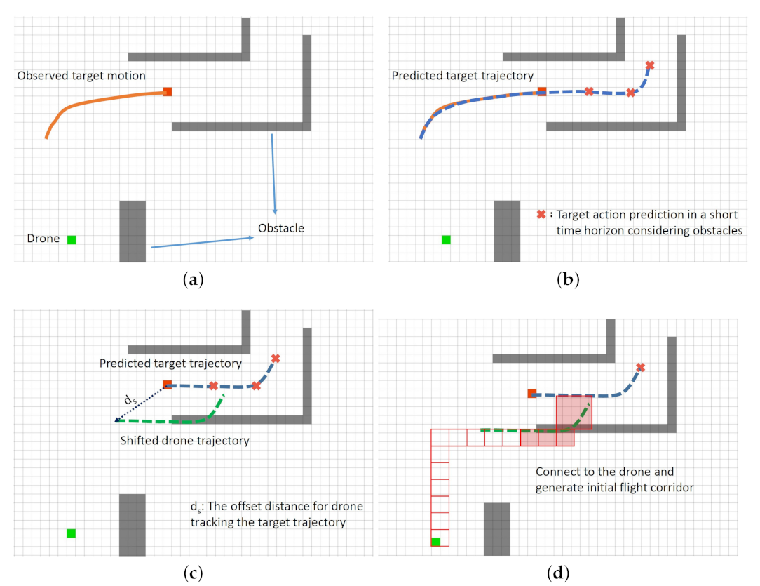
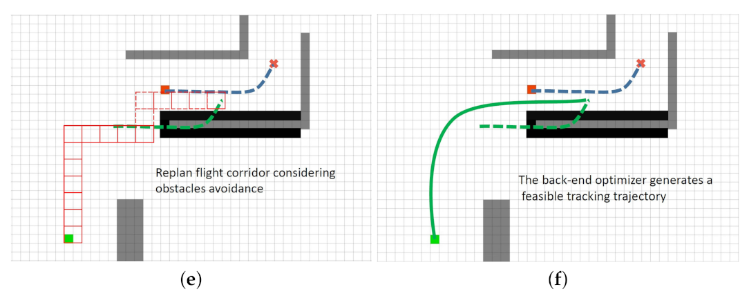
The octree structure is an efficient technique for representing obstacle information in the environment, which stores the obstacle information in a 3D cubic grid of variable size. Figure 2 describes the flow of the target tracking trajectory planning algorithm. Firstly, the approach uses onboard sensors to observe the current position and historical trajectory of the target (Figure 2a), then predicts the target’s moving position in the future by analyzing the distribution of obstacles around the target. The polynomial is applied to fit the approximate target trajectory (Figure 2b). Next, the estimated target trajectory is offset along the d s direction to obtain a rigid trajectory of target tracking, which usually interferes with obstacles (Figure 2c). After that, using the map grid path traversed by the rigid tracking trajectory, the initial flight corridor of the UAV can be formed (Figure 2d). However, the flight corridor could not meet the safety requirements, the multi-start A* algorithm is used to adjust the interference part to find a collision-free go-around corridor (Figure 2e). This flight corridor is connected with the current position of the drone, then the A* algorithm is used to generate a safe tracking flight corridor for the drone. Finally, in the case of satisfying the dynamic constraints, a QP-based method was adopted to optimize the safe and dynamically feasible tracking trajectories (Figure 2f).

3. Target Motion Estimation and Prediction

In this section, we first introduce the target motion estimation and prediction method based on the distribution of obstacles, and then explain the relocation rule after the tracking target is lost.

3.1. Target Path Prediction

According to the previous assumption, the target motion is smooth. The Bézier curve could fit the target motion well, so this paper uses the Bézier curve to depict the target prediction trajectory. The n-degree Bézier curve can be expressed as
B ( t ) = i = 0 n w i h n i ( t ) ,
where each h n i is the basis of the polynomial, [ w 0 , w 1 , , w n ] is the set of control points of the Bézier curve.
The relative position of the target and the UAV can be observed utilizing the onboard sensor, then when the position of the UAV is known, the observation sequence of the target position with noise interference in the global frame can be obtained through coordinate transformation. t L is defined as the current time, t 1 is the start time of the sliding window, and there are L observations during the time period [ t 1 , t L ] . In this paper, the 3D position of the target at time t R is denoted as p ( t ) R 3 , the value of the Euclidean signed distance field at a position p of the prior map is defined as ϕ ( p ) . A fixed-input fixed-output vector of length L is then obtained, which stores historical observations and corresponding timestamps of the target. This vector is represented as Q = [ q 1 , q 2 , , q L ] , where q i = [ p t i , t i ] .
This paper designs a weight factor w t i to distinguish the confidence of observations at each time. It can be expressed as
w t i = f t i = tanh c t t L t i , ( i = 1 , 2 , , L 1 ) 1 , ( i = L ) .
The credibility of observations with different timestamps cannot be treated equally. The older the target observation value, the lower the reference significance for target prediction. Obviously its weight in the cost function should be relatively small. As the time difference between t i and the current time t L increases, the value of hyperbolic tangent function t a n h ( x ) decreases rapidly. This mathematical property can be effectively applied in the calculation of confidence levels for different observations.
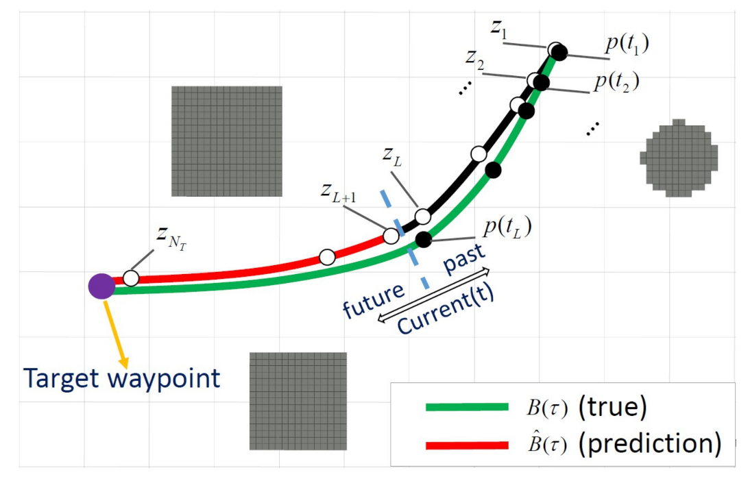
In the target prediction algorithm, the UAV collects historical observations of the target at discrete time points t 1 , t 2 , , t L . The target then goes to the target waypoint for a short time, which is calculated considering the area that the target can reach in a period of time τ and distribution of obstacles around the target. To predict the target’s future trajectory B ^ ( τ ) , the algorithm designs a discrete position path ξ = { z 1 , z 2 , , z N T } ( z i R 3 and N T > L ) that covers the target’s past observations and the predicted path between the current position and the waypoint. Considering that the target will effort to avoid obstacles, simultaneously in order to avoid overfitting, an obstacle avoidance adjustment term and an acceleration adjuster are added to the cost function to guarantee the security and smoothness of the predicted target trajectory. The optimization formula B ^ ( τ ) is expressed as follows
min ξ i = 1 L w t i B ^ t i p i 2 2 estimation residual + L λ t t l t m B ^ ( 2 ) ( t ) 2 2 d t acceleration regulator + λ f n = 1 N T f o b s ( z n ) obstacle ,
where λ t is used to adjust the weighting of the regulator; λ f is used to adjust the effect of obstacles on position prediction; t m is the time limit for predicting the target trajectory; [ t 1 , t L ] is the time period during which the target observation is actually performed; [ t L , t m ] is the short time range for predicting the target motion. The prediction is used to generate the tracking trajectories. The second term implies that the target will minimize its derivatives and the efficiency of its ego-motion. The integral of the l 2 norm of the polynomial has a quadratic closed form, so the second term is a constraint-free QP, which has a closed form solution [40]. The function f o b s is used to explain the behavioral principle of the target. Under the condition of satisfying dynamic feasibility, the target tends to move forward the free space. It is a non-convex cost function inherited from ϕ ( p ) , which can be solved through the scheme in [41]. Equation (3) can be organized into a standard form for covariant optimization as
min ξ 1 2 ρ A ξ b 2 prior term + f o b s ( ξ ) obstacle term .
Equation (4) can be solved with Δ ξ = α A T A 1 ρ A T A ξ A T b + f o b s ( ξ ) , where α is the step size.
As shown in Figure 3, a geometric path ξ is obtained from Formulas (1)–(4), where z L + 1 , , z N T represents the prediction of the target from current target position to the waypoint. These discrete waypoints can be used to complete the target trajectory prediction.

3.2. Time Prediction

To reduce computational complexity, each point z i in ξ is assigned a time node t i and is specified to have a constant velocity. The historical observation points of the target z n ( n L ) do not need too many constraints, simply assign observation timestamps. The following rule is used to allocate the times for predicted locations z n ( n > L ) .
t n = t n 1 + z n z n 1 v ¯ ,
where v ¯ = n = 1 L 1 x p , n x p , n + 1 t L t 1 indicates the average velocity of the acquired observations. That is to say, the transit time of the point in Formula (3) can be estimated based on the constant velocity v ¯ . With this time allocation strategy, the future trajectory of the target in the time window ( t , t + H ] can be predicted with the interpolation
B ^ ( τ ) = t n + 1 τ z n + τ t n z n + 1 t n + 1 t n t n < τ < t n + 1 .
To show the real-time performance of the proposed approach, the frequency of a single prediction optimization routine is set to a minimum of 15 Hz, which helps to find relatively inexpensive trajectories. Thanks to the existence of the obstacle avoidance item f o b s , the approach can find better prediction results based on the obstacle distribution.

3.3. Target Relocate

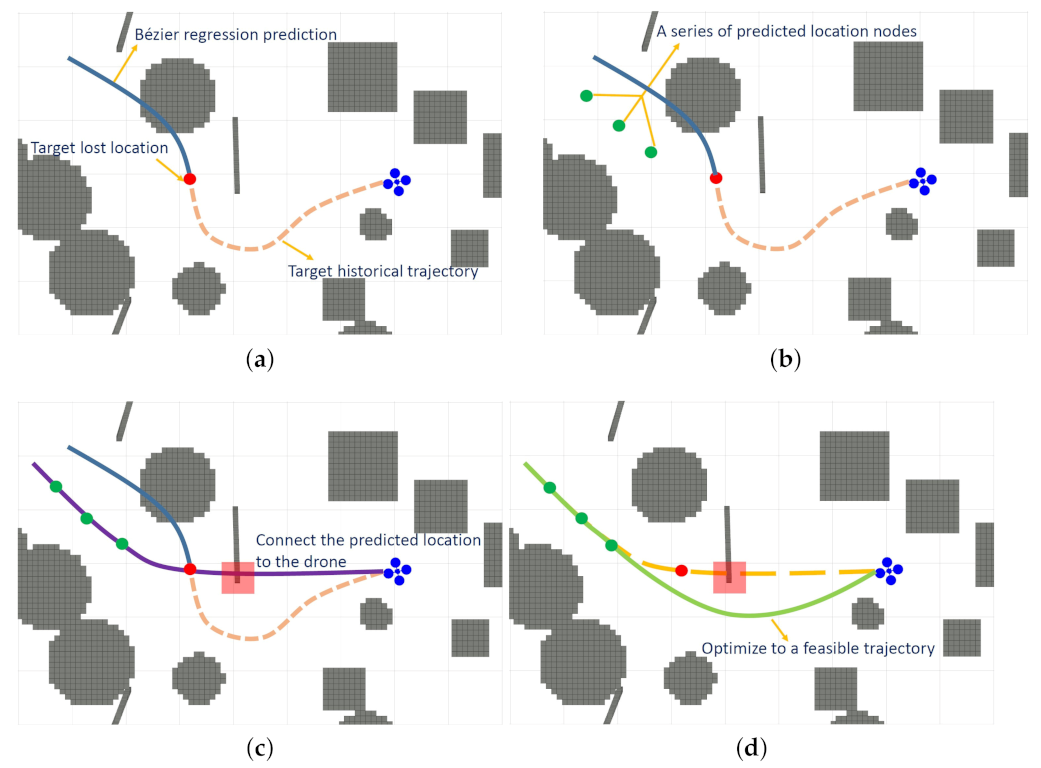
When the UAV tracks the movement of the target, it is inevitable that the tracking target will be lost due to the occlusion of obstacles. Generally, the drone will call the sensor to search for the target location after reaching the last target observation point, but this rigid method sometimes has significant limitations. This paper proposes an effective strategy to enable UAVs to respond quickly while losing targets, and actively exploring and relocating the targets by predicting the target trajectory. The detailed process design is illustrated in Figure 4.
The predicted trajectory in Figure 4a is generated with Bézier regression. When not considering the obstacles around the target, the predicted trajectory may interfere with the obstacles. The target relocation strategy proposed in this paper can avoid similar problems. Firstly, the loss of the target causes the relocation mechanism to be triggered. By analyzing the surrounding environment of the last target observation point, combined with the target prediction algorithm mentioned above, the predicted position of the target within a period of time can be obtained (Figure 4b). Then to generate a flight corridor (Figure 4c), the predicted trajectory of the target is connected with the current position of the UAV. Based on the flight corridor, the tracking trajectory can be further optimized. During relocalization, if new obstacles are observed on the tracked trajectory, the backend optimizer will regenerate a safe and dynamically feasible tracking trajectory (Figure 4d). Compared with the Bézier regression prediction, the proposed strategy analyzes the surrounding environment of the target lost point when predicting the target. The target prediction result is more accurate so that the system resource can be used more in the subsequent relocation work.

4. Safe Tracking Trajectory Planning

This section introduces the safe tracking trajectory planning scheme, which includes target-informed dynamic tracking path searching and spatial–temporal optimal trajectory generation.

4.1. Dynamic Tracking Path Searching

Hybrid A* algorithm [42] is an efficient, practical, and widely used algorithm, which extends the nodes generated by the discretized control input to search for safe and dynamically feasible trajectories. The dynamic search method proposed in this paper is based on it, then a heuristic function is designed, which can make full use of the target prediction trajectory to quickly search the target tracking trajectory.
The state of UAV is represented as a vector x = ( p x , p y , p z , v x , v y , v z ) T . The acceleration is denoted as the control input u u : = [ a m p , a m p ] 3 R 3 . Then u is discretized as u N : = a m t , n a 1 n a a m t , , n a 1 n a a m t , a m t in each dimension. The expansion duration is denoted as Δ T : = 1 n t Δ T m , 2 n t Δ T m , n t 1 n t Δ T m , Δ T m . The state transition equation can be represented as follows:
x k = 1 Δ T 0 1 x k 1 + 1 2 Δ T 2 Δ T u N ,
where x k 1 represents the previous state. Given x k 1 , u N , and Δ T , motion primitives can be generated by expanding the nodes. At most, ( 2 n a + 1 ) 3 · n t motion primitives can be generated in a single expansion process.
The cost function of a node is expressed as f c = g c + h c , where g c denotes the actual cost from the initial state x 0 to the current state x c , h c represents the heuristic cost, which makes searching faster. The energy-time cost function is mainly related to the control-effort and the time of a trajectory, the proposed method trades off these two factors by minimizing them. The energy-time cost function is expressed as follows:
J t ( T ) = 0 T u ( τ ) 2 d τ + ρ T .
The motion primitives are generated by the discretized input u N and Δ T in a single expansion process. Then the cost of a motion primitive can be represented as e c = u N 2 + ρ Δ T . Therefore, assuming there are m motion primitives that make up the optimal path x 0 to x c , g c can be determined as
g c = i = 1 m e i = i = 1 m u N i 2 + ρ Δ T i .
The heuristic function h c can significantly accelerate the search speed of the algorithm, which consists of two parts and is expressed as follows:
h c = D x c , x g + W t H t t c ,
where D x c , x g represents the Euclidean distance from the current state of the UAV x c to the destination state x g . To make the search results forward-looking, this paper adopts the weighted value of x t c and x t p instead of the goal state x g to yield
x g = ( 1 σ ) x tc + σ x tp ,
where σ represents the weight. x tp propagates along B ^ ( t ) in the wake of the increasing path expansion time τ . In this paper, the time axis of the path expansion process is designed to synchronize with the target predicted trajectory. To be specific, at time τ of the path expansion, x t p ( τ ) = p t p , v t p = B ^ ( τ ) , B ^ ( 1 ) ( τ ) .
The minimum dynamic cost of an optimal path is solved by an optimal boundary value problem (OBVP) proposed in [43]. Based on this method, the paper defines the OBVP distance D x c , x g for the question under study, which is the minimum cost solved by the problem between x c and x g .
For another, W t ( H t τ ) is design as a time penalty term, where W t represents the weight and H t denotes the sum of expected expansion time. The original intention of introducing this term is to trade off the optimality and computational efficiency, but the experiment shows that it greatly speeds up the search velocity of the algorithm. It makes the algorithm prefer to choose the adjacent region of the current node, rather than the whole state space. Since the search area is greatly reduced, the algorithm runs much faster. The results verify that planners can find satisfactory solutions in most scenarios.

4.2. Spatial–Temporal Optimal Trajectory Generation

The optimization algorithm proposed in [37] expresses the tracking trajectory by piecewise polynomials. In this paper, a back-end trajectory optimizer is designed based on this method, which optimizes the intermediate waypoints q w and the piece time T of piecewise polynomial trajectories. The method cleverly reduces the optimization variables involved, which makes it possible to generate a spatiotemporal optimal trajectory p ( t ) in a given flight corridor. Firstly, a flight corridor F is generated according to the trajectory obtained from the front end analysis, which can be represented as follows:
F = i = 1 M C i ,
where each C i = x R 3 A c i x b c i represents a finite cube. F is used as the input to minimize the cost function
J Σ q w , T = J S q w , T + J F q w + J D q w , T .
The one-dimensional smoothness cost J S ( q w , T ) is denoted as follows:
J S μ = i = 1 M 0 T i p i μ ( 3 ) ( t ) 2 d t .
This logarithmic barrier term J F ( q w ) is designed as
J F q w = υ i = 1 M 1 j = i i + 1 E T ln b c j A c j q w i ,
where υ is a constant coefficient, E is denoted as an all-ones vector and ln [·] is the entry-wise natural logarithm. This term could guarantee that each q w i is constrained in C i C i + 1 . J D ( q w , T ) is designed as a penalty to adjust the aggressiveness of the whole tracking trajectory, it can be expressed as
J D q w , T = ρ t i = 1 M T i + ρ v i = 1 M 1 ι q w i + 1 q w i 1 T i + 1 + T i 2 v m 2 + ρ a i = 1 M 1 ι q w i + 1 q w i / T i + 1 q w i q w i 1 / T i T i + 1 + T i / 2 2 a m 2 ,
where ι ( x ) = m a x ( x , 0 ) 3 , v m and a m are, respectively, the maximum velocity and maximum acceleration of the tracker.
In the algorithm, in the schematic diagram shown in Figure 5, the black part represents the obstacles in the environment, and the distance between the target and the obstacles will have a cascade change on the trajectory cost. The closer the distance from the obstacle, the higher the collision probability of the UAV. The proposed algorithm tends to predict the position of the target in the range of time τ in the safe area, which mainly trades off the dynamic consumption and the path hazard to generate a series of predicted target nodes. The green curve represents the target predicted trajectory, the red curve indicates the expansion process of the UAV. The details of the proposed algorithm are shown in Algorithm 1.
Algorithm 1: Trajectory searching for dynamic tracking.
 Input: openlist Φ o , closelist Φ c , current node n c , predicted trajectory B ^ ( t ) , initial state X 0 , goal state X g .
 Output: Target tracking trajectory F .
1:initialization ()
2:while Φ o is not empty do
3:     n c ← FindMinCostNode( Φ o )
4:     X g ← GenerateGoal( n c , B ^ ( t ) )
5:    if Reach( n c , X g ) or AnalyticExpand( n c , X g ) Then
6:        return OptimalSearchPath()
7:    end if
8:        Φ c .push_back( n c )
9:        n o d e s ← Expand( n c )
10:       for n i in n o d e s  do
11:             X g ← GenerateGoal( n i , B ^ ( t ) )
12:      if Nofeasible( n c , n i ) or n i Φ c  Then
13:         continue
14:        end if
15:         g o n c .g+EdgeCost ( n c , n i )
16:        if n i Φ o Then
17:            Φ o .push_back( n i )
18:       else if g o > n i . g Then
19:              continue
20:         end if
21:          n i . p a r e n t n c
22:          n i . g g o
23:          n i . f n i . g +Heuristic( n i , X g )
24:    end for
25: end while
26: return Target tracking trajectory F

5. Numerical Case Study

In this section, we conduct a large number of simulation experiments on the proposed approach in a variety of different scenarios. We then compare the experimental results with state-of-the-art methods in the field. The results demonstrate that the proposed algorithm has strong robustness and high efficiency, and it has excellent performance in target movement prediction and safe trajectory generation.

5.1. Implementation Details

We validated the proposed algorithm in multiple dense environments. For the simulation, we used a complex city model, which included multiple non-convex obstacles; the target moved freely and autonomously and hid behind the obstacles. In the simulation experiment, the target was set as a freely moving car. In order to be detected by sensors, the car was equipped with a recognizable tag. The visual fiducial system proposed in [44] ws used to detect the tag. In addition, to enhance the perception range of the system, we configured three cameras to form a broad field-of-view camera array. The target detection sensor had a range of 10 m and a field of view of 120 degrees. With credit given to the broad view, the drone did not have to struggle to maintain a relative angle to the target. Meanwhile, the algorithm correspondingly planned the tangential direction of the UAV motion to ensure a safe flight. For the sake of verifying the effectiveness of the proposed approach, we equipped a laptop with an Intel i7 CPU and 16 GB RAM, the replanning frequency of the approach was set to 15 Hz, the simulation experiments were performed in RVIZ under the ROS development environment.

5.2. Experimental Results

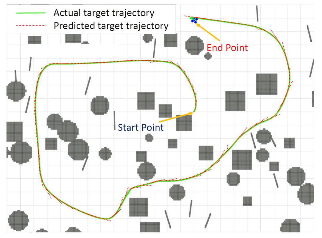
We presented several aggressive and safe aerial tracking experiments in cluttered environments, as shown in Figure 6. The proposed algorithm has obvious advantages in the face of complex environments. By identifying the distribution of obstacles, it can predict the intent of the target well, which provides more time for the back-end optimization of the trajectory.
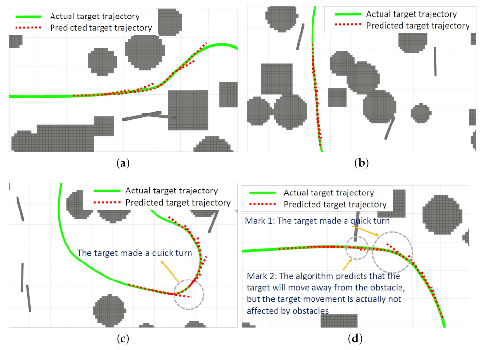
The back-end optimizer (attributed to the efficient effect of the target prediction algorithm) obtained more optimization time; therefore, the UAV could track moving targets safely and smoothly in these challenging environments. The excellent performance of the proposed approach was verified in a variety of complex scenarios. As shown in Figure 7a, in a complex environment, the closer the target was to the obstacle, the greater the danger to the target. Under the principle of ensuring the safety of the trajectory and minimum costs, the algorithm was inclined to predict that the target would advance along the direction with minimum costs. The tight distribution of obstacles conversely provided a safe corridor range for target prediction, and made the prediction results more accurate in the complex environment I.
In another complex environment II shown in Figure 7b, the obstacles were enclosed to form a corridor that was similar to a straight line. Although the target could move freely, there were no other choices in the forward direction. The proposed algorithm also made a rather excellent prediction of the target movement, which verified its excellence.
However, in some open areas, due to the absence of obstacle threats and the consideration of minimum costs, the algorithm tended to predict that the target would remain in the current state, and did not predict the sudden and large movement changes of the target in time. In the open environment I shown in Figure 7c, the target movement had high safety in all directions due to few surrounding obstacles. Since the target had free intentions, there was more uncertainty in the choice of the moving route. In this environment, the proposed algorithm was based on the consideration of the minimum cost of the path, and tended to predict that the target kept moving in the current state. It was difficult to predict the sudden large-scale movement change of the target in time shown in the circle mark.
Similarly, in another open environment II shown in Figure 7d, the algorithm predicted that the target would keep going straight at circle mark 1, but the target executed a large change in direction. At circle mark 2, the algorithm predicted that the target would move away from the obstacle, but the target actually moved and did not deliberately avoid the obstacle. This was not because the algorithm was inaccurate, but the target had the ability to move freely.
The more constrained the environment, the smaller the moving space range of the target. This is why the algorithm performed better in a complex environment. Although there were more choices for target movements in the open area, the algorithm could not predict some rapid and large direction changes of the target in advance. Moreover, as few factors threatened the flight safety of the drone in this environment, the drone had greater flexibility in adjusting the tracking trajectory, which did not drastically reduce the tracking performance.

5.3. Benchmark Comparisons

In order to show the excellence of our proposed research method, we compared the target motion prediction method and the tracking trajectory planner described in this paper with the cutting-edge methods in the field. The baseline environment was built over an area of 25 × 25 × 3.5 m, which contained 180 randomly generated obstacles with various shapes and structures.
Firstly, we compared the difference between the actual future moving position of the target and the predicted result with [4]. Since the path planner in [4] is quite different from the design principle proposed in this paper, there is no comparison significance. In order to quantify the difference terms, we took advantage of the average distance error e ¯ between the future target position p f ( t ) and the predicted trajectory P ^ ( t ) . e ¯ can be computed by
e ¯ = i = 1 L f P ^ t c + i · t s p f t c + i · t s 2 L f ,
where t c denotes the current time, t s = 0.05 s represents the sample interval, and L f = 50 expresses the sampling size. During the observation, the ground truth of the target location is often disturbed by Gaussian noise with zero means. To this end, we designed three gradually increasing noise levels to show the contrast effects. Gaussian noise with standard deviations of 0.05, 0.3, and 0.6 m represent low noise, medium noise, and high noise environments, respectively. The common parameter for the two comparison methods was set to ( n = 5 , L = 30 , t p t L = 2.5 s , w p = 15 ) . To reduce the impact of chance errors, more than 20,000 target motion predictions were generated in each environment.
Compared with the method in [4] at different levels of noise interference environments, the proposed target motion prediction method had significant advantages on the average distance error as shown in Figure 8. The computation time of the proposed method was approximately 0.5 ms, while that of the method [4] was about 0.3 ms. Both methods showed high performance in computational speed. Although the proposed method took a little longer (regarding computation time), the prediction accuracy was improved by at least 40%, which verified the practicability of the proposed algorithm. It is obvious that the proposed target motion prediction method is more accurate and reliable.
Afterward, we compared our work with [4] in terms of the tracking trajectory planner. The target moved freely through the scenario in each simulated tracking task. In order to objectively compare the two planners, the actual position of the target future trajectory was directly provided as input. In order to quantify the comparative results of these two methods, some quantitative indicators were developed in this paper. We propose a concept called effective tracking time, in which the distance between the UAV and the target in the x y plane is less than 3 m before it can be counted as an effective tracking time. Meanwhile, we designed the tracking rate r t , which is the ratio of the effective tracking time to the total tracking time. In order to highlight the performance differences between the two planners, we set different difficulty-tracking scenarios. The computation time and r t are compared in 200 tracking missions for each scenario.
From Table 1, it can be seen that, compared with method [4], our proposed planner not only occupies much lower computing resources, but also achieves better tracking effects. It shows strong robustness and efficiency. This is attributed to the high-frequency replanning of the proposed planner, which can make it react better in some extreme situations, such as a sudden turn or acceleration of the target.

6. Conclusions and Future Work

This paper presents a safe and efficient system for UAVs to track dynamic moving targets in complex environments. Extensive experiments and benchmark comparisons have confirmed the robustness and efficiency of the proposed approach. The approach is mainly composed of two modules: target motion prediction and path searcher. In the target motion prediction module, we used the Bézier regression to predict the future movement of the target based on the distribution of obstacles around the target and past observations. The experimental results demonstrated that the proposed method is excellent in dealing with complex scenes with high accuracy and efficiency. However, in some open environments, the algorithm cannot timely predict the extreme motions of the target, such as approaching obstacles or suddenly turning around. However, this problem can be solved by the path searcher mentioned later. In order to obtain safe tracking trajectories in complex scenes, this paper proposes a heuristic dynamic searcher, which can generate safe and dynamically feasible tracking trajectories based on a previous target motion prediction. The excellent performance of the searcher can be observed from the benchmark comparison results.
In the future, we will focus on the multi-angle tracking of multiple UAVs to a single target and the formation flight of multiple drones. In addition, we will explore more practical object recognition methods, so that the proposed approach could be applied to more diversified scenes.

Author Contributions

Conceptualization, S.C., Y.C. and X.L.; methodology, S.C. and Y.C.; software, S.C. and Y.C.; validation, S.C. and Y.C.; formal analysis, S.C. and Y.C.; investigation, S.C. and Y.C.; resources, S.C., Y.C. and X.L.; data curation, Y.C.; writing—original draft preparation, S.C.; writing—review and editing, Y.C. and X.L.; visualization, S.C., Y.C. and X.L.; supervision, Y.C. and X.L.; project administration, Y.C. and X.L.; funding acquisition, Y.C. and X.L. All authors have read and agreed to the published version of the manuscript.

Funding

This research was funded by the Open Fund of the Key Laboratory of Civil Aircraft Airworthiness Technology (grant no. SH2020112703) and the National Natural Science Foundation of China (grant no. 62103293).

Institutional Review Board Statement

Not applicable.

Informed Consent Statement

Not applicable.

Data Availability Statement

Not applicable.

Conflicts of Interest

The authors declare no conflict of interest.

Abbreviations

The following abbreviations are used in this manuscript:
UAVunmanned aerial vehicle
QPquadratic programming
ESDFEuclidean signed distance field
OBVPoptimal boundary value problem

References

  1. Shen, S.; Mulgaonkar, Y.; Michael, N.; Kumar, V. Vision-Based State Estimation and Trajectory Control Towards High-Speed Flight with a Quadrotor. Robot. Sci. Syst. 2013, 1. [Google Scholar] [CrossRef]
  2. Goodarzi, F.A.; Lee, D.; Lee, T. Geometric adaptive tracking control of a quadrotor unmanned aerial vehicle on SE (3) for agile maneuvers. J. Dyn. Syst. Meas. Control 2015, 137, 091007. [Google Scholar] [CrossRef] [Green Version]
  3. Mellinger, D.; Michael, N.; Kumar, V. Trajectory generation and control for precise aggressive maneuvers with quadrotors. Int. J. Robot. Res. 2012, 31, 664–674. [Google Scholar] [CrossRef]
  4. Ge, P.; Chen, Y.; Wang, G.; Weng, G. An active contour model driven by adaptive local pre-fitting energy function based on Jeffreys divergence for image segmentation. Expert Syst. Appl. 2022, 210, 118493. [Google Scholar] [CrossRef]
  5. Penin, B.; Giordano, P.R.; Chaumette, F. Vision-based reactive planning for aggressive target tracking while avoiding collisions and occlusions. IEEE Robot. Autom. Lett. 2018, 3, 3725–3732. [Google Scholar] [CrossRef] [Green Version]
  6. Ge, P.; Chen, Y.; Wang, G.; Weng, G. A hybrid active contour model based on pre-fitting energy and adaptive functions for fast image segmentation. Pattern Recognit. Lett. 2022, 158, 71–79. [Google Scholar] [CrossRef]
  7. Liu, S.; Watterson, M.; Mohta, K.; Sun, K.; Bhattacharya, S.; Taylor, C.J.; Kumar, V. Planning dynamically feasible trajectories for quadrotors using safe flight corridors in 3-d complex environments. IEEE Robot. Autom. Lett. 2017, 2, 1688–1695. [Google Scholar] [CrossRef]
  8. Chen, Y.; Cheng, C.; Zhang, Y.; Li, X.; Sun, L. A Neural Network-Based Navigation Approach for Autonomous Mobile Robot Systems. Appl. Sci. 2022, 12, 7796. [Google Scholar] [CrossRef]
  9. Bošnak, M.; Matko, D.; Blažič, S. Quadrocopter hovering using position-estimation information from inertial sensors and a high-delay video system. J. Intell. Robot. Syst. 2012, 67, 43–60. [Google Scholar] [CrossRef]
  10. Cheng, C.; Chen, Y. A Neural Network based Mobile Robot Navigation Approach using Reinforcement Learning Parameter Tuning Mechanism. In Proceedings of the 2021 China Automation Congress (CAC), Beijing, China, 22–24 October 2021; pp. 2600–2605. [Google Scholar]
  11. Teuliere, C.; March, E.; Eck, L. 3-D model-based tracking for UAV indoor localization. IEEE Trans. Cybern. 2014, 45, 869–879. [Google Scholar] [CrossRef] [PubMed]
  12. Martínez, C.; Mondragón, I.F.; Olivares-Méndez, M.A.; Campoy, P. On-board and ground visual pose estimation techniques for UAV control. J. Intell. Robot. Syst. 2011, 61, 301–320. [Google Scholar] [CrossRef] [Green Version]
  13. Gomez-Balderas, J.E.; Flores, G.; García Carrillo, L.R.; Lozano, R. Tracking a ground moving target with a quadrotor using switching control. J. Intell. Robot. Syst. 2013, 70, 65–78. [Google Scholar]
  14. Weiss, S.; Achtelik, M.W.; Lynen, S.; Achtelik, M.C.; Kneip, L.; Chli, M.; Siegwart, R. Monocular vision for long-term micro aerial vehicle state estimation: A compendium. J. Field Robot. 2013, 30, 803–831. [Google Scholar] [CrossRef]
  15. Dong, J.; Mukadam, M.; Dellaert, F.; Boots, B. Motion planning as probabilistic inference using gaussian processes and factor graphs. Robot. Sci. Syst. 2016, 12. [Google Scholar] [CrossRef]
  16. Kim, J.; Shim, D.H.; Morrison, J.R. Tablet PC-based visual target-following system for quadrotors. J. Intell. Robot. Syst. 2014, 74, 85–95. [Google Scholar] [CrossRef]
  17. Azrad, S.; Kendoul, F.; Nonami, K. Visual servoing of quadrotor micro-air vehicle using color-based tracking algorithm. J. Syst. Des. Dyn. 2010, 4, 255–268. [Google Scholar] [CrossRef] [Green Version]
  18. Liu, F.; Wei, Z.; Zhang, G. An off-board vision system for relative attitude measurement of aircraft. IEEE Trans. Ind. Electron. 2021, 69, 4225–4233. [Google Scholar] [CrossRef]
  19. Knuth, C.; Chou, G.; Ozay, N.; Berenson, D. Planning with learned dynamics: Probabilistic guarantees on safety and reachability via lipschitz constants. IEEE Robot. Autom. Lett. 2021, 6, 5129–5136. [Google Scholar] [CrossRef]
  20. Ohnishi, M.; Wang, L.; Notomista, G.; Egerstedt, M. Barrier-certified adaptive reinforcement learning with applications to brushbot navigation. IEEE Trans. Robot. 2019, 35, 1186–1205. [Google Scholar]
  21. Chen, Y.; Zhou, Y. Machine learning based decision making for time varying systems: Parameter estimation and performance optimization. Knowl.-Based Syst. 2020, 190, 105479. [Google Scholar] [CrossRef]
  22. Chen, H.; Liu, Z.; Alippi, C.; Huang, B.; Liu, D. Explainable Intelligent Fault Diagnosis for Nonlinear Dynamic Systems: From Unsupervised to Supervised Learning. IEEE Trans. Neural Netw. Learn. Syst. 2022. [Google Scholar] [CrossRef] [PubMed]
  23. Chen, Y.; Zhou, Y.; Zhang, Y. Machine learning-based model predictive control for collaborative production planning problem with unknown information. Electronics 2021, 10, 1818. [Google Scholar] [CrossRef]
  24. Chen, H.; Jiang, B.; Ding, S.X.; Huang, B. Data-driven fault diagnosis for traction systems in high-speed trains: A survey, challenges, and perspectives. IEEE Trans. Intell. Transp. Syst. 2021, 23, 1700–1716. [Google Scholar] [CrossRef]
  25. Liu, X.; Yang, Y.; Ma, C.; Li, J.; Zhang, S. Real-time visual tracking of moving targets using a low-cost unmanned aerial vehicle with a 3-axis stabilized gimbal system. Appl. Sci. 2020, 10, 5064. [Google Scholar] [CrossRef]
  26. Chen, Y.; Chu, B.; Freeman, C.T. Generalized iterative learning control using successive projection: Algorithm, convergence, and experimental verification. IEEE Trans. Control Syst. Technol. 2020, 28, 2079–2091. [Google Scholar] [CrossRef] [Green Version]
  27. Chen, Y.; Chu, B.; Freeman, C.T. Iterative learning control for path-following tasks with performance optimization. IEEE Trans. Control Syst. Technol. 2021, 30, 234–246. [Google Scholar] [CrossRef]
  28. Cui, S.; Chen, Y.; Tao, H. An Automatic Approach for Aircraft Landing Process Based on Iterative Learning Control. In Proceedings of the 2022 IEEE 11th Data Driven Control and Learning Systems Conference (DDCLS), Chengdu, China, 3–5 August 2022; pp. 531–536. [Google Scholar]
  29. Chen, Y.; Chu, B.; Freeman, C.T. Iterative Learning Control for Robotic Path Following with Trial-Varying Motion Profiles. IEEE/ASME Trans. Mechatron. 2022. [Google Scholar] [CrossRef]
  30. Nägeli, T.; Alonso-Mora, J.; Domahidi, A.; Rus, D.; Hilliges, O. Real-time motion planning for aerial videography with dynamic obstacle avoidance and viewpoint optimization. IEEE Robot. Autom. Lett. 2017, 2, 1696–1703. [Google Scholar]
  31. Penin, B.; Spica, R.; Giordano, P.R.; Chaumette, F. Vision-based minimum-time trajectory generation for a quadrotor UAV. In Proceedings of the 2017 IEEE/RSJ International Conference on Intelligent Robots and Systems (IROS), Vancouver, BC, Canada, 24–28 September 2017; pp. 6199–6206. [Google Scholar]
  32. Chen, Y.; Jiang, W.; Charalambous, T. Machine learning based iterative learning control for non-repetitive time-varying systems. Int. J. Robust Nonlinear Control 2022. [Google Scholar] [CrossRef]
  33. Fu, C.; Lin, F.; Li, Y.; Chen, G. Correlation filter-based visual tracking for UAV with online multi-feature learning. Remote Sens. 2019, 11, 549. [Google Scholar] [CrossRef] [Green Version]
  34. Bonatti, R.; Zhang, Y.; Choudhury, S.; Wang, W.; Scherer, S. Autonomous drone cinematographer: Using artistic principles to create smooth, safe, occlusion-free trajectories for aerial filming. In Proceedings of the International Symposium on Experimental Robotics, Buenos Aires, Argentina, 5–8 November 2018; Springer: Cham, Switzerland, 2018; pp. 119–129. [Google Scholar]
  35. Li, S.; Ozo, M.M.; De Wagter, C.; de Croon, G.C. Autonomous drone race: A computationally efficient vision-based navigation and control strategy. Robot. Auton. Syst. 2020, 133, 103621. [Google Scholar] [CrossRef]
  36. Richter, C.; Bry, A.; Roy, N. Polynomial trajectory planning for aggressive quadrotor flight in dense indoor environments. In Robotics Research; Springer: Cham, Switzerland, 2016; pp. 649–666. [Google Scholar]
  37. Foehn, P.; Romero, A.; Scaramuzza, D. Time-optimal planning for quadrotor waypoint flight. Sci. Robot. 2021, 6, eabh1221. [Google Scholar] [CrossRef] [PubMed]
  38. Garrido-Jurado, S.; Muñoz-Salinas, R.; Madrid-Cuevas, F.J.; Marín-Jiménez, M.J. Automatic generation and detection of highly reliable fiducial markers under occlusion. Pattern Recognit. 2014, 47, 2280–2292. [Google Scholar] [CrossRef]
  39. Shen, S.; Michael, N.; Kumar, V. Obtaining liftoff indoors: Autonomous navigation in confined indoor environments. IEEE Robot. Autom. Mag. 2013, 20, 40–48. [Google Scholar] [CrossRef]
  40. Boyd, S.; Enberghe, L. Convex Optimization; Cambridge University Press: Cambridge, UK, 2004. [Google Scholar]
  41. Rickert, M.; Sieverling, A.; Brock, O. Balancing exploration and exploitation in sampling-based motion planning. IEEE Trans. Robot. 2014, 30, 1305–1317. [Google Scholar] [CrossRef]
  42. Dolgov, D.; Thrun, S.; Montemerlo, M.; Diebel, J. Practical search techniques in path planning for autonomous driving. Ann Arbor 2008, 1001, 18–80. [Google Scholar]
  43. Zhou, B.; Gao, F.; Wang, L.; Liu, C.; Shen, S. Robust and efficient quadrotor trajectory generation for fast autonomous flight. IEEE Robot. Autom. Lett. 2019, 4, 3529–3536. [Google Scholar] [CrossRef] [Green Version]
  44. Huang, J.K.; Wang, S.; Ghaffari, M.; Grizzle, J.W. LiDARTag: A real-time fiducial tag system for point clouds. IEEE Robot. Autom. Lett. 2021, 6, 4875–4882. [Google Scholar] [CrossRef]
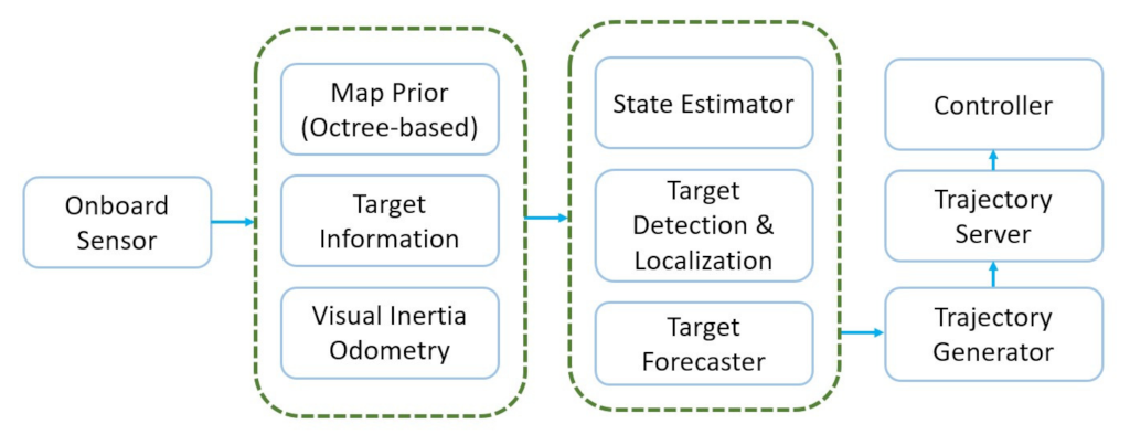
Figure 1. UAV path planning approach architecture diagram.
Machines 10 00931 g001
Figure 2. Graphical illustration of the algorithmic pipeline. (a) Observe the target trajectory by the onboard sensor. (b) Predict the target trajectory considering nearby obstacles. (c) Offset along the d s vector to generate rigid target tracking trajectories. (d) Connect to the drone and generate initial flight corridor. (e) Generate the re-planned flight corridor considering obstacles avoidance. (f) The back-end optimizer generates a feasible tracking trajectory.
Machines 10 00931 g002aMachines 10 00931 g002b
Figure 3. The prediction of the target motion.
Machines 10 00931 g003
Figure 4. The expanded description of the relocation strategy. (a) The target motion prediction based on the Bézier regression interferes with the nearby obstacle. (b) The proposed target motion prediction considers the obstacles around the target lost point. (c) The predicted trajectory of the target and the current position of the UAV are connected to generate a flight corridor. (d) The backend optimizer regenerates a safe and dynamically feasible flight trajectory.
Machines 10 00931 g004
Figure 5. An illustration of the dynamic tracking path searching method.
Machines 10 00931 g005
Figure 6. Active and safe aerial tracking experiment in a complex environment.
Machines 10 00931 g006
Figure 7. Performance of the proposed prediction algorithm in a variety of scenarios. (a) Performance of the proposed prediction algorithm in complex environment I. (b) Performance of the proposed prediction algorithm in complex environment II. (c) Performance of the proposed prediction algorithm in open environment I. (d) Performance of the proposed prediction algorithm in open environment II.
Machines 10 00931 g007
Figure 8. Target motion prediction method comparison.
Machines 10 00931 g008
Table 1. Tracking trajectory planner comparison in multiple complex situations.
ScenarioMethod t front (ms) t back (ms) t total  (ms) r t (%)
v ¯ = 1.2 m/sProposed5.81.16.997.3
v m = 2.3 m/sMethod [4]222.711.3234.091.4
v ¯ = 1.6 m/sProposed11.61.613.292.1
v m = 3.0 m/sMethod [4]240.511.4251.985.1
v ¯ = 2.1 m/sProposed14.92.516.986.3
v m = 3.9 m/sMethod [4]363.810.9274.769.3
Publisher’s Note: MDPI stays neutral with regard to jurisdictional claims in published maps and institutional affiliations.