Tool Remaining Useful Life Prediction Method Based on Multi-Sensor Fusion under Variable Working Conditions

Abstract

Under variable working conditions, the tool status signal is affected by changing machine processing parameters, resulting in a decreased prediction accuracy of the remaining useful life (RUL). Aiming at this problem, a method based on multi-sensor fusion for tool RUL prediction was proposed. Firstly, the factorization machine (FM) was used to extract the nonlinear processing features in the low-frequency condition signal, and the one-dimensional separable convolution was applied to extract tool life state features from multi-channel high-frequency sensor signals. Secondly, the residual attention mechanism was introduced to weight the low-frequency condition characteristics and high-frequency state characteristics, respectively. Finally, the features extracted in the low-frequency and high-frequency parts were input into the full connection layer to integrate working condition information and state information to suppress the influence of variable conditions and improve prediction accuracy. The experimental results demonstrated that the method could predict the remaining life of the tool effectively, and the accuracy and stability of the model are better than several other methods.

1. Introduction

As one of the major components which directly contact with the workpiece in the whole machining system, the health state of the tool is particularly important to ensure the machining accuracy of high-end equipment. If the tool cannot be changed in time before the tool life is exhausted, it is easy to cause additional power consumption [1,2], reduce the quality of the workpiece, and even lead to blade collapse or tool breaking and cause serious production accidents and personnel damage. Therefore, accurate prediction of tool remaining useful life (RUL) is of great significance for improving the productivity and production quality of the workpiece.

In recent years, machine learning-based tool life prediction has attracted wide attention from researchers, such as support vector machine [3,4,5], correlation vector machine [6], hidden Markov model (HMM) [7], and Bayesian [8] and artificial neural networks [9,10,11]. However, these methods often require the construction of health indicators made out of the time and frequency domain characteristics of the original signal [12,13,14] or obtained through the signal decomposition method [15,16,17,18,19,20]. As a result, the quality of the selected features depends on the prior knowledge of the signal processing technology and specific prediction conditions, and have poor generalization. Moreover, manual features are usually extracted from the entire range of time-series data, which may not capture its intrinsic temporal information and limit the ability of neural networks to learn complex nonlinear relationships in tool RUL prediction application.

Deep learning can directly automatically extract deep features from the raw signal and mine the hidden information behind the data through the deep network, overcoming the shortcomings of the above prediction methods. Liu et al. [21] proposed a novel tool wear monitoring model based on parallel residual and stacked bidirectional long and short-term memory networks (BiLSTM) to achieve high prediction accuracy without sacrificing its generalization ability. Zhang et al. [22] proposed a hybrid model integrating residual structure and BiLSTM for tool wear monitoring to solve the problem of gradient disappearance and degradation during life prediction. However, the tool status information contained in a single sensor is limited, which limits the further improvement of model performance.

As different sensor signals can provide complementary information in the feature space, to improve the tool RUL prediction accuracy, some scholars have conducted the tool life prediction research based on multi-sensor fusion. For example, Gao et al. [23] proposed a new time–space attention mechanism driven multi-feature fusion method for tool wear monitoring and residual useful life prediction, which can more accurately capture the complex spatio-temporal relationship between tool wear values and features to predict wear values. Cheng et al. [24] integrated a new framework of feature normalization, attention mechanism and residual network algorithm for tool wear monitoring and multi-step prediction, which has great advantages in efficiency and robustness compared with other data-driven models. Xu et al. [25] used the parallel convolutional neural net-work to perform multi-scale feature fusion in the parallel convolutional neural network and combined this with the channel attention mechanism of residual connections to improve the performance of the model. These prediction results of tool wear are more robust and accurate than the methods based on single sensor.

Although the above deep learning-based tool RUL prediction methods have achieved some results, these methods still have the following problems:

• The influence of the changing working condition in the tool RUL prediction has not been considered. Most current studies only focus on constant working condition, and there are few prediction methods for tool RUL under variable conditions.
• Most of the existing studies simultaneously use multiplex sensors as input data to predict the tool RUL, but not all the sensor signals are conducive to the tool RUL prediction, and the contribution of different sensors to the tool prediction results is not considered. As a result, the model obtains limited tool degradation information and has poor prediction performance.

For the above problems, this paper proposed a variable working condition tool residual life prediction method based on low frequency working condition signal and high frequency multi-sensor state signal fusion, called factorization machine and separable convolution network with residual attention (FMRA_SCNRA). First, the model is divided into two parts: a low frequency working condition signal and a high frequency multi-sensor signal. The factorization machine (FM) is used to extract the nonlinear features and perform the feature fuses with the residual attention mechanism. Secondly, the high-frequency multi-sensor signal is divided into multi-channel signal, and the features are extracted automatically using one-dimensional separable convolution, respectively, by weighing each channel through the residual attention mechanism. Finally, the two-part extracted features are spliced as the input vector of the neural network for training and learning to obtain the tool remaining lifetime percentage. The main contributions of this article include:

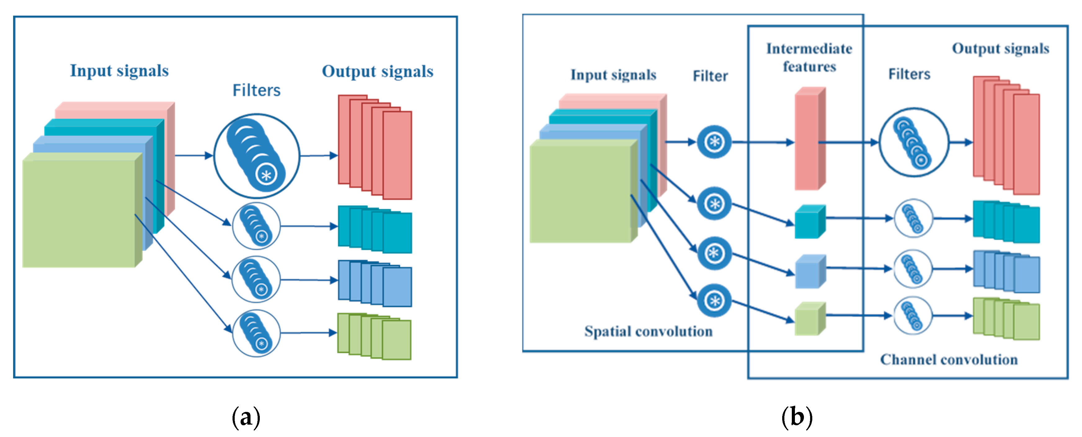
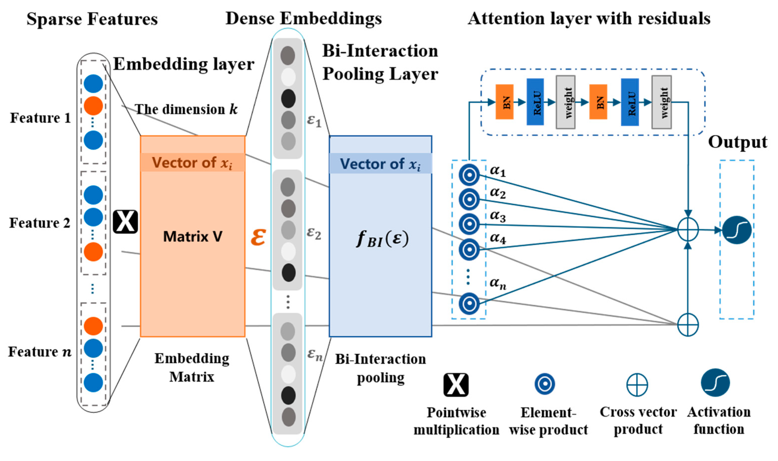
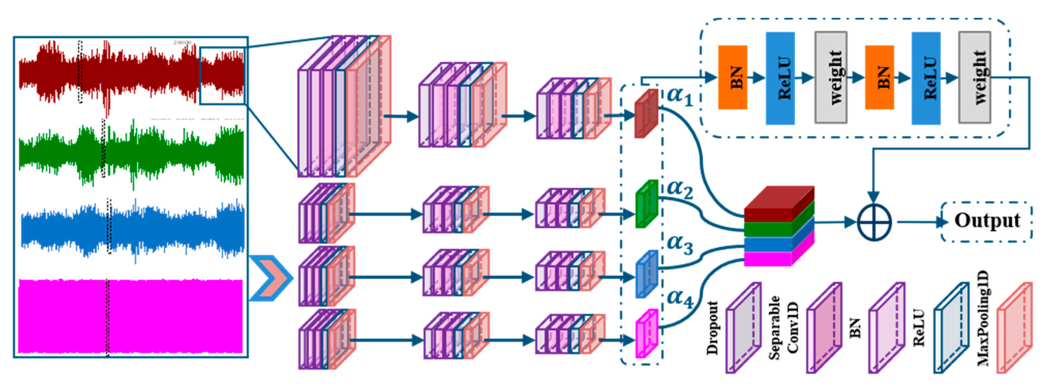
• The factorization machine is used to extract the nonlinear processing characteristics in the low-frequency working condition signal, and the one-dimensional separable convolution layer is extracted in the multi-channel high-frequency sensor signal. The model integrates the working condition signal and the high-frequency sensor state information.
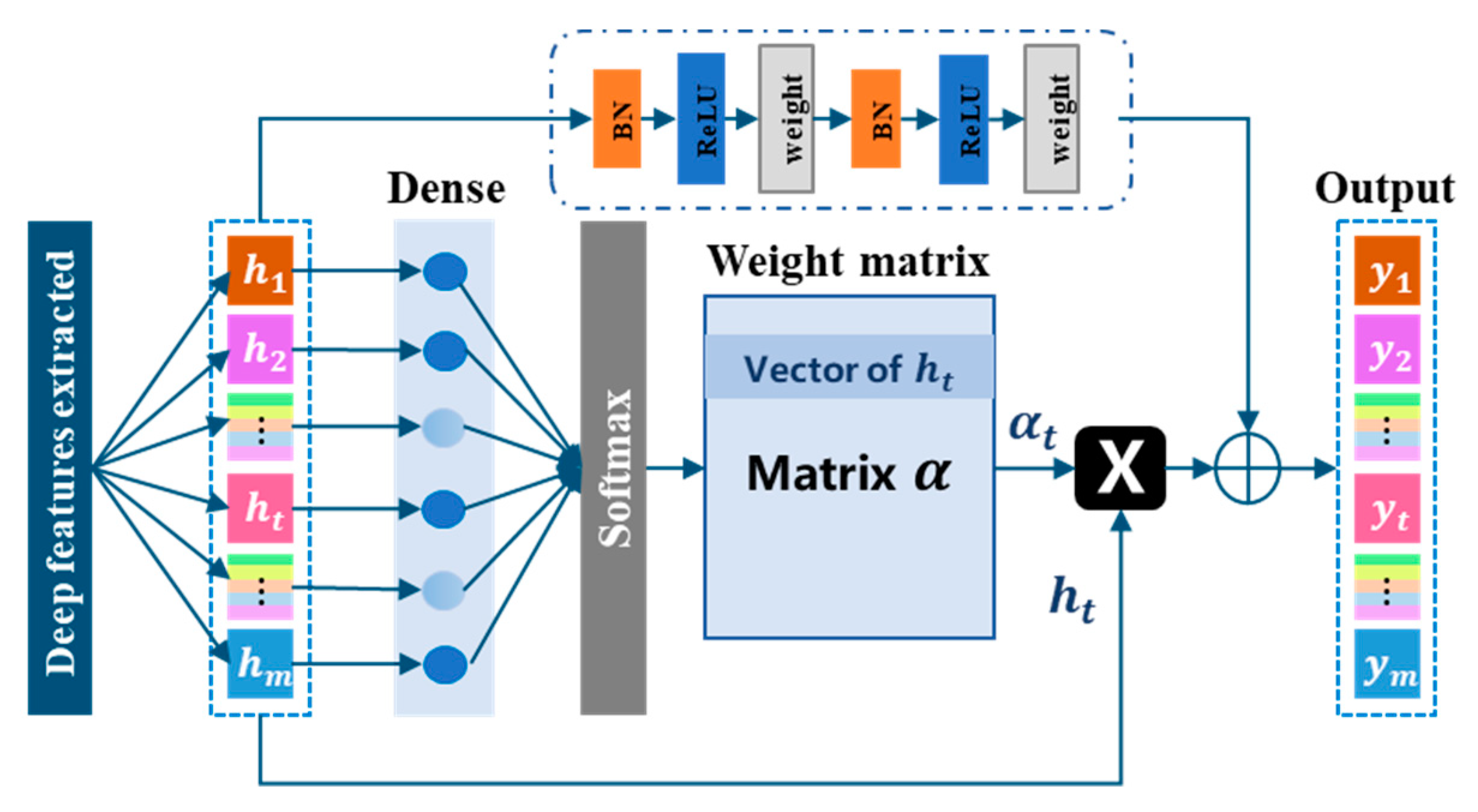
• The attention mechanism with residual differences was applied to integrate features and fuse these features with the adaptive weight determined weights from different signals, which can transmit low-level features to the high level to avoid the upper-level bottleneck problem caused by network degradation.
• Using Foxconn’s publicly available data set for experimental verification and analysis, experiments prove that the proposed method can effectively improve the prediction accuracy and stability of the model.

The rest is organized as follows: Section 2 introduces related theory, the details of the proposed method are described in Section 3, Section 4 shows the experimental studies and the results, and finally, Section 5 concludes this work.

2. Related Theory

The calculation of ordinary convolutions is a joint mapping of both spatial and channel convolutions. When computing the multi-channel input, each channel of the convolution kernel and each channel of the input respectively perform the convolution operation to directly obtain the characteristics of the multichannel, as shown in Figure 1a. The parameters of each convolutional network are determined by using a learnable kernel, which is convolved with the output $c_j^{i-1}$ of the ($l-1$)th layer. The results obtained serve as the input of the next layer, which can be expressed as:

$$c_j^{(l)}=f({\displaystyle {\sum }_{i\in M_j}{\omega }_{i,j}^{(l)}\cdot c_i^{(l-1)}+b_j^{(l)}})$$

(1)

where $c_j^{(l)}$ is the $j$th feature map of the $l$th layer, $c_i^{(l-1)}$ is the $i$th feature map of the ($l-1$)th layer, ${\omega }_{i,j}^{(l)}$ and $b_j^{(l)}$ are the weight and bias of the convolution kernel, $M_j$ denotes the $j$th convolution region of the ($l-1$)th layer, and $f(·)$ is the activation function.

The calculation process of separable convolution is different, which divides the ordinary convolution calculation process into two parts: spatial convolution and channel convolution. First, a channel of the convolution kernel is spatially convoluted with each channel of the input to obtain the intermediate features of multiple channels. Then, this multi-channel intermediate feature tensor performs the channel convolution operation of multiple 1 × 1 convolution kernels to obtain multiple height-width-invariant outputs. It can be seen that the separated convolutional layer contains two steps of convolution operations, while the first step is a single convolution kernel, and the second one contains multiple convolution kernels, as shown in Figure 1b. One-dimensional separable convolution greatly reduces the number of parameters and computation, improving the system performance and the speed of model training.

3. Tool RUL Prediction Method Based on Multi-Sensor Fusion under Variable Operating Conditions

In the process of workpiece processing, the tool state signal is easily affected by the working conditions. Meanwhile, different sensor signals have different prediction contributions to the tool life. If these two issue are not fully considered, it will seriously impact the performance of tool RUL prediction under variable working conditions.

To solve the above problems, this paper presents a tool residual life prediction method based on FMRA_SCNRA. First, FM is used to extract nonlinear features of low-frequency working condition signals and fuse features with attention mechanisms with residuals. Secondly, separable convolution is used to automatically extract deep features of multichannel sensor signals and fuse multiplex features with an attention mechanism with residue. Finally, the two parts of advanced features are input into the full connection layer to output the tool RUL prediction results.

3.1. The FMRA_SCNRA Overall Framework

The overall structure of the FMRA_SCNRA network is shown in Figure 2, which mainly consists of two parts of the network branches to perform feature extraction and fusion of processing signals and sensor signals, respectively. Due to the inconsistent sampling frequency of the two-part inputs, in order to realize the data time synchronization, the processing signal and the sensor signal of the same time period are taken as the input at the moment, and the low-frequency processing signal also becomes highly sparse. The raw time-series data of the machine tool processing is used as an input to the FMRA_SCNRA network, and then used as an input to the FMRA after data preprocessing and normalization. The FMRA is used to extract and fuse the sparsity of working condition data characteristics due to excessive sampling frequency difference. The raw time series acquired by the sensor underwent grouping, data preprocessing, and normalization as another input to the FMRA_SCNRA network, which is the input to the SCNRA. Multi-sensor deep features were extracted by constructing one-dimensional separable convolutional modules and fused by a residual attention mechanism. Finally, the fused features of the two networks are merged as input from three fully connected layers to predict the RUL of the tool.

3.2. FMRA Network Fusion Working Condition Information

The FMRA network uses a method based on DeepFM [26] to process signals with sparse characteristics, improves the FM by introducing different importance to different kinds of FM features interaction, and the importance is learned through the attention mechanism, and the proposed residual attention mechanism is adopted here, as shown in Figure 3.

Let the conversion $X=[x_1,x_2,\dots ,x_n]$ of the raw signal feature component from sparse input to dense vector is embedding structure. Where $n$ is the length of the data sample, and the training data has a corresponding target value. Based on the defects of FM, this paper improves the structure of the feature interaction pooling layer, proposing to adopt a residual attention mechanism for the feature interactions by weighting the interaction vectors and retaining the low-level features. The formula is derived as follows:

The output of FM is the sum of an additive unit and multiple inner product units, with the formula:

$${\widehat{y}}_{\mathrm{FM}}(X)=w_0+{\displaystyle {\sum }_{i=1}^n{w}_i{x}_i+{\displaystyle {\sum }_{i=1}^n{\displaystyle {\sum }_{j=i+1}^n\langle V_i,V_j\rangle }}}{x}_i{x}_j$$

(2)

where $w_0$ is the global deviation, $w_i$ is the weight of the $i$th feature. The output of the Embedding layer is:

$$\epsilon =\left\{v_1{x}_1,v_2{x}_2,\dots ,v_n{x}_n\right\},x_i\ne 0$$

(3)

Here ${\epsilon }_i=({\epsilon }_{i1},{\epsilon }_{i2},\dots ,{\epsilon }_{ik})$ represents an embedding vector, and $k$ is the dimension. The feature interaction pooling layer introduces this set of embedding vector $\epsilon$ and feature component $X$ for Hadamard product calculation to complete the feature interaction, and the output is:

$$f_{BI}(\epsilon )={\displaystyle {\sum }_{i=1}^n{\displaystyle {\sum }_{j=i+1}^n{x}_i{v}_i\odot }}{x}_j{v}_j$$

(4)

where $\odot$ is the Hadamard product.

The residual attention $f_{BI}(\epsilon )$ is used to perform adaptive matching weights of the feature interaction pool vector and retain the original features, and the output is:

$$f_{RA}(f_{BI}(\epsilon ))={\displaystyle {\sum }_{i=1}^n{\displaystyle {\sum }_{j=i+1}^n{\alpha }_{ij}(x_i{v}_i\odot }}{x}_j{v}_j)+{\displaystyle {\sum }_{i=1}^n{\displaystyle {\sum }_{j=i+1}^n{f}_{RES}(x_i{v}_i\odot }}{x}_j{v}_j)$$

(5)

where ${\alpha }_{ij}$ is the attention weight of the feature interaction, which can be obtained from the attention mechanism network, and $f_{RES}(·)$ indicates that the residual calculation is performed for each interaction feature. Therefore, the output of the FMRA network is:

$${\widehat{y}}_{\mathrm{FMRA}}(X)=w_0+{\displaystyle {\sum }_{i=1}^n{w}_i{x}_i}+f_{RA}(f_{BI}(\epsilon ))$$

(6)

3.3. The SCNRA Network Integrates Multi-Sensor Information

The SCNRA network designs a parallel one-dimensional separable convolutional deep network architecture to fuse the multi-channel sensor features, as shown in Figure 4. First, deep features are extracted by constructing three one-dimensional separable convolutional modules consisting of the five-layer neural networks of the dropout layer, the SeparableConv1D, the batch normalization layer, the rectified linear (ReLU) activation function, and MaxPooling1D layer. The designed parallel one-dimensional separable convolutional module operation can separately extract features from different signals collected by multiple sensors. Then, the extracted features use the attention mechanism adaptation to assign different weights for splicing, and the low-level features are transmitted to the post splicing features through the residual network. It not only preserves the low-level features to prevent the network degradation caused by the increase of network layers but also solves the problem of differences in different sensor features and improves the accuracy of model prediction.

3.4. Residual Attention Network

In the fusion step, the features extracted from the working condition data and the multi-sensor data are fused using the residual attention mechanism module (RA) proposed here, as shown in Figure 5. The extracted deep features are denoted by the expression $H=\left[h_1,h_2,\dots ,h_m\right]$, where $m$ is the number of channels of the proposed feature. Due to the different influence degree of different deep features on the tool RUL, this module can not only adaptively assign weights to the extracted depth features but also prevent the network degradation so that the low-level features can also be transmitted to the high-level features to express the training effect.

Firstly, pass deep feature $h_t$ into the full connection layer output $u_t$ with tanh activation function with the following formula:

$$u_t=\tanh (W{h}_t+b)$$

(7)

where $h_t$ is the extracted depth feature, the $W$ and $b$ denote the corresponding weights and bias matrices. The transpose of the output multiplied by the trainable parameter vector $u$ yields the alignment coefficient of attention $\exp (u_t^{T}u)$.

Secondly, the softmax function is used to normalize the alignment coefficient, obtain the sum-adaptive weight ${\alpha }_t$, and express the weighted sum of the calculated deep features with vector ${\widehat{y}}_{Attention}$. The formula is as follows:

$${\alpha }_t=\mathrm{softmax}(u_t)=\frac{\exp (u_t^{T}u)}{{\displaystyle {\sum }_{t=1}^n\exp (u_t^{T}u)}}$$

(8)

$${\widehat{y}}_{Attention}={\displaystyle {\sum }_{t=1}^n{\alpha }_t{h}_t}$$

(9)

Thirdly, the residual network with a fully pre-activated structure constructed by He [27] is used to improve the network generalization ability and reduce the overfitting, and the output is expressed by the vector ${\widehat{y}}_{Residual}$ as:

$${\widehat{y}}_{Residual}=f_{RES}(h_t)=\psi (h_t,W_q)=Dense(\mathrm{ReLU}(W_q(BN(\xi ))+b_q))$$

(10)

where BN is batch normalization, $\xi =Dense(\mathrm{ReLU}(W_{q-1}(BN(h_t))+b_{q-1}))$. $W_q$ and $b_q$ are the weight and bias of the $q$th layer in the residual network.

Finally, the summed fusion output of the two vectors is expressed as ${\widehat{y}}_{RA}$:

$${\widehat{y}}_{RA}={\widehat{y}}_{Attention}+{\widehat{y}}_{Residual}={\displaystyle {\sum }_{t=1}^m{\alpha }_t{h}_t}+Dense(\mathrm{ReLU}(W_q(BN(\xi ))+b_q))$$

(11)

4. Process of Tool RUL Prediction Based on Multi-Sensor Fusion under Variable Operating Conditions

Figure 6 presents the procedure for using the tool RUL prediction method based on FMRA_SCNRA. It includes data acquisition, pre-processing and normalization, model construction and training, and test samples for model prediction validation.

• Data acquisition, preprocessing, and normalization: different signals are collected from the CNC machine tools through multiple sensors, and the operating condition signals are collected through the PLC. The collected data were then preprocessed, including data cleaning, [0, 1] wide normalization.
• Model construction and training: After building the model, the training samples are trained, and the network parameters are adjusted through indicators and visual analysis.
• Model prediction validation: the test samples after pre-processing and normalization are input to the trained model for validation, and the prediction effect of the model is verified through comparative experiments.

5. Experimental Validation

5.1. Introduction of the Experimental Dataset

The experimental data of this paper is the relevant data of the “tool remaining life prediction” competition in the second Industrial Big Data Innovation Competition, which is truly processed and collected by Foxconn CNC Machine Tool. The schematic diagram of the experimental device is shown in Figure 7 with installing XYZ acceleration sensor near the end surface of the spindle. The information physical fusion system framework is used to collect the three-phase vibration signal and the synchronous current signal of the same frequency at the sampling frequency of 25,600 Hz, and the controller signal is collected at the sampling frequency of 33 Hz, including the working condition information such as the three-direction axis (x, y, z) mechanical coordinates and spindle load. These data are obtained from the machining procedure of a brand-new tool until the end of the tool life, providing only a one-minute fragment every five minutes as a training sample, provided by the time series 1.csv, 2.csv,…, n.csv. The tool 1 example is specifically described in

Table 1. The description of tool 1 acquisition signal.

File Type	Sampling Frequency	Number of Files	Data	Describe
Sensor data	25,600 Hz	48	vibration_1	x-axis vibration signal
			vibration_2	y-axis vibration signal
			vibration_3	z-axis vibration signal
			current	First phase current
PLC data	33 Hz	1	time	Record time
			spindle_load	Spindle load
			x	x-axis coordinate
			y	y-axis coordinate
			z	z-axis coordinate
			csv_no	Number of corresponding Sensor _files

. In this paper, the data of the whole tool life cycle provided by the platform is used as training data, and the full life cycle of the three tools are 240 min, 240 min, and 185 min, respectively, and the other tool with a local time period (70 min–120 min) is used as test data to verify the performance of the proposed model.

5.2. Data Preprocessing

After data acquisition, it is found that the spindle load has no empty files, and the collected sample point of the downtime period and the corresponding sensor_file should be deleted, as shown in Figure 8. In Figure 8a, the signal in the three red boxes represent the signals collected during shutdown, which cannot be used for model training and need to be deleted; the deleted signals are shown in Figure 8b. According to the machining mechanism of the machine tool, the spindle load can reflect the cutting force or cutting depth of the machining tool wear trend, so it is used as a variable working condition signal. Then adopt group alignment to make time synchronization, namely every 776 high frequency data sampling point and 1 low frequency sampling point combined to generate a sample, and take a sample per 10 samples to reduce the amount of data, and the experiment has no effect on prediction accuracy, but the training time is faster than no down sampling more than 100 times. In addition, due to the inconsistent working life of tools, simply using the remaining working minutes as the label cannot visually reflect the tool wear state. Therefore, the concept of “tool remaining life ratio” (RULR) is proposed here, with the remaining life divided by the total life of the tool as the label of the data, which can actually characterize the tool RUL more. The effective time (CL) already spent by the tool and the effective time interval (CLI) already spent by the tool are also calculated and then combined with the spindle load to form the processed sample collection. The sensor sample collection is composed of grouped multi-channel sensors. Together, both samples constitute the input to the model.

5.3. Model Parameter Setting

As shown from

Table 2. The parameter settings of three-layer 1D separable convolution-pooling module.

Layer	Type	Parameter Setting 1	Output Size
1	Dropout 1	0.5	(n, 776, 1)
2	SeparableConv1D 1	32, 11, 1	(n, 776, 32)
3	Batch Normalization 1		(n, 776, 32)
4	Activation 1	ReLU	(n, 776, 32)
5	MaxPooling1D 1	11	(n, 71, 32)
6	Dropout 2	0.5	(n, 71, 32)
7	SeparableConv1D 2	64, 9, 1	(n, 71, 64)
8	Batch Normalization 2		(n, 71, 64)
9	Activation 2	ReLU	(n, 71, 64)
10	MaxPooling1D 2	9	(n, 8, 64)
11	Dropout 3	0.5	(n, 8, 64)
12	SeparableConv1D 3	128, 7, 1	(n, 8, 128)
13	Batch Normalization 3		(n, 8, 128)
14	Activation 3	ReLU	(n, 8, 128)
15	MaxPooling1D 3	7	(n, 2, 128)

¹ Note: The “Parameter Setting” column is the parameters corresponding to the layer of neural network, where the parameter order of one-dimensional separable convolution is: filter size/convolution kernel size/step size.

, the feature extraction framework consists of two parts. The working condition part is composed of a layer of FM to obtain the feature cross pool vector, and performs the feature fusion with the applicable RA of the linear part. Since the CLI represents the interval as relatively sparse, both are treated as sparse features, and spindle_load and CL as dense features. The dimension of the embedding vector was set to 4, the regularization coefficient of the linear part was set to ${10}^{-5}$, the regularization sparsity of the embedding vector was set to ${10}^{-5}$, the random seed as 1024, and the learning task as regression.

The sensor part consists of three layers of one-dimensional separable convolutional-pooling module and residual attention, with the activation function of ReLU, and the dimensional transformation and parameter settings are shown in Table 2. The batch normalization technology allows us to use higher learning rates, and it acts as a regularization, and the dropout can prevent the overfitting phenomenon. The residual part adopts the structure of Figure 5. The difference is that weight is fully connected in the fusion condition, and convolution is used in the fusion sensor. Here, the convolution core size is 7, the step length is 1, and the number of filters is consistent with the input. The last two parts of spliced inputs into three fully connected layers predicted the tool RUL, the neurons were set to 256, 128, 1, respectively, and the activation function to ReLU. In addition, the average absolute error (MAE) is selected as the loss function of the training, and the adaptive moment estimation (Adam) is used as the optimization algorithm of the model, and the early stop method is used to obtain the optimal model. The number of early stop steps is set to 11 steps. The number of model training times was 100, and the batch size per incoming model training was 128.

5.4. Experimental Results and Comparative Analysis

To verify the effectiveness of the proposed method for tool RUL prediction, the FMRA_SCNRA is compared with four different methods: (1) the separable convolution network (SCN), (2) the factorization machine and separable convolution network (FM_SCN), (3) the residual attention based factorization machine and separable convolution network (FMRA_SCN), and (4) the factorization machine and residual attention based separable convolution network (FM_SCNRA) The similarities and dissimilarities of the four methods are shown as below:

(1)

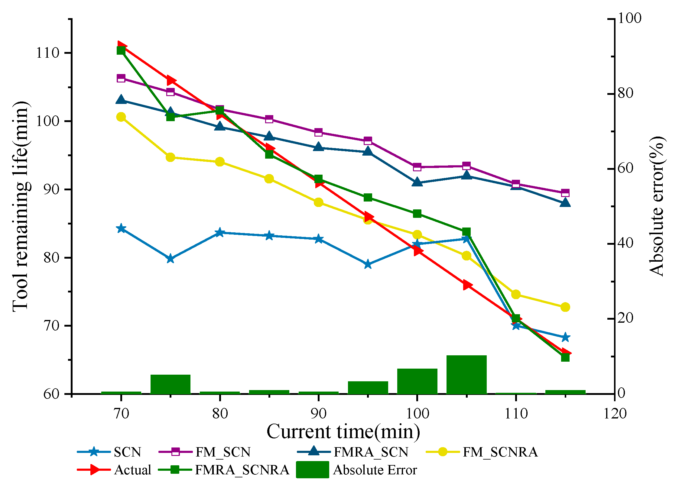
SCN: only uses three layers of concurrent one-dimensional separable convolutional module to extract the multi-sensor features and then directly merge the input into the three layers of fully connected layer;

(2)

FM_SCN: uses the same SCN to extract multi-sensor features, the FM network is also used to extract the working condition features, Then, the two-part features are combined and input into the three fully connected layers;

(3)

FMRA_SCN: based on FM_SCN model and use the adaptive weight allocation of residual attention mechanism on the extracted operating features;

(4)

FM_SCNRA: based on the FM_SCN model and using the residual attention mechanism on the extracted sensor features. In the contrast experiments, modeling the same branching network parameters remained consistent.

In order to ensure the fairness of comparison, the network parameter settings of the same part of each model are consistent. All experiments were performed under Python 3.8.8 and framework Tensorflow-2.2.0, run on a computer with the CPU i5-10400F, GPU GTX 1650 and 16 GB RAM. The preprocessed test data is input into different life prediction models for tool RUL prediction. The test data are another new tool dataset with a 70 min–120 min difference from the training set. The life prediction results under different methods are shown in Figure 9. It can be intuitively seen from the figure that the overall trend of the tool RUL can be predicted, which proves the feasibility of the proposed multi-channel sensor model structure considering the working condition information. Moreover, the FMRA_SCNRA model has obvious advantages in prediction accuracy and stability. The comparison shows that the FM_SCN, FMRA_SCN models fit well the tool RUL trends in the early stage, but their predictive power decreases significantly when the tool wear is dramatically changed in the later stage. The FM_SCNRA model is better for the late fitting tool RUL. This shows that the residual attention module enhances the ability to fuse deep features and model convergence to prevent network degradation. By assigning the residual attention network to the sensor and working condition features, respectively, and retaining the original features, FMRA_SCNRA can more accurately monitor the tool RUL, and the remaining tool life is closer to the real life of the tool.

In order to evaluate the prediction performance of the model quantitatively and intuitively, the average absolute error (MAE), root mean square error (RMSE), and accuracy are introduced to evaluate the prediction accuracy of the model, and the peak-to-peak value (P-P value) is used to evaluate the stability of the model. The four evaluation indicators are shown in the formula: (12)–(15), and the comparative analysis results of the different methods are shown in

Table 3. The comparison of tool RUL prediction evaluation indicators under different methods.

Index	MAE	RMSE	Accuracy (%)	P-P Value
SCN	11.91	13.92	87.93	26.58
FM_SCN	10.28	12.71	88.05	23.46
FMRA_SCN	9.80	11.91	88.65	21.93
FM_SCNRA	5.34	6.27	94.31	11.30
FMRA_SCNRA	2.48	3.59	97.18	7.78

.

$$\mathrm{MAE}=\frac{1}{N}{\displaystyle {\sum }_{i=1}^N\left|E{r}_i\right|}$$

(12)

$$\mathrm{RMSE}=\sqrt{\frac{1}{N}{\displaystyle {\sum }_{i=1}^{N}E{r}_i{}^2}}$$

(13)

$$\mathrm{Accuracy}=\frac{1}{N}{{\displaystyle {\sum }_{i=1}^N\exp }}^{-\frac{\left|E{r}_i\right|}{RU{L}_{Rea{l}^{(i)}}}}$$

(14)

$$\mathrm{P}\text{-}\mathrm{P}\mathrm{value}=\max (E{r}_i)-\min (E{r}_i)$$

(15)

where $N$ represents the number of samples, the error of the $i$ sample is represented by the following formula:

$$E{r}_i=RU{L}_{Rea{l}^{(i)}}-RU{L}_{predictio{n}^{(i)}}$$

(16)

Experiments show that the FMRA_SCNRA model shows a high accuracy and a good stability for the tool RUL prediction. According to Table 3, the MAE, RMSE, and peak-to-peak values are all the largest for the SCN without taking the working condition into consideration. Compared with FM_SCN, MAE added working condition information reduced by 1.63, RMSE reduced by 1.21, accuracy improved by 0.12%, and peak value reduced by 3.12, indicating that working condition has a certain impact on tool RUL. Although FMRA_SCN method is adaptively weighted fused through residual attention network, the weight allocation effect of method is not obvious due to the sparsity of the working condition data. Compared with FM_SCN, the method improves the accuracy and stability of tool RUL prediction less. However, the FM_SCNRA method, MAE, reduced 4.94, RMSE reduced 6.44, accuracy improved 6.26%, and peak value decreased 12.16, which significantly improved the prediction accuracy and stability. The main reason is that the FM_SCNRA method performs the feature-weighted fusion of the sensor signal with sufficient data quantity and adds the residual difference to prevent the network degradation, which improves the prediction accuracy of the model to a certain extent, but its effect is worse than that of the FMRA_SCNRA method. The FMRA_SCNRA method has the smallest prediction error and the smallest peak value after the residual attention fusion in both parts, indicating that the dual-input network structure and the residual attention feature fusion device proposed by this method can effectively predict the tool RUL. The main reason is that the FMRA_SCNRA method also solves the multi-sensor performance tool degradation characteristics of different conditions and the variable condition signal, and the experimental results show that the accuracy and stability indexes are better than the other models, which verifies the effectiveness of the proposed method in this paper.

6. Conclusions

The prediction of tool RUL under variable conditions is important. Compared with the traditional deep learning method, this paper proposes a tool RUL prediction method integrating factorization machine, residual attention, and separable convolution for the problem of different tool degradation characteristics and variable working condition signals driving tool life. It can not only extract features from the original multi-channel sensor signal and the working condition signal respectively at the same time but also improve the quality of feature fusion and avoid the degradation of the deep network through residual attention. The experimental results show that the proposed FMRA_SCNRA method is closer to the actual life curve, with the high degree of fit, the minimum prediction error of MAE and RMSE, the highest accuracy, and the best peak prediction stability, which proves the effectiveness of the proposed method and provides a new idea for the tool remaining life prediction under variable conditions.

References

1. Colantonio, L.; Equeter, L.; Dehombreux, P.; Ducobu, F. A Systematic Literature Review of Cutting Tool Wear Monitoring in Turning by Using Artificial Intelligence Techniques. Machines 2021, 9, 351. [Google Scholar] [CrossRef]
2. Kumar, R.; Sahoo, A.K.; Mishra, P.C.; Das, R.K. Measurement and Machinability Study under Environmentally Conscious Spray Impingement Cooling Assisted Machining. Measurement 2019, 135, 913–927. [Google Scholar] [CrossRef]
3. Benkedjouh, T.; Medjaher, K.; Zerhouni, N.; Rechak, S. Health Assessment and Life Prediction of Cutting Tools Based on Support Vector Regression. J. Intell. Manuf. 2015, 26, 213–223. [Google Scholar] [CrossRef] [Green Version]
4. Kong, D.; Chen, Y.; Li, N.; Tan, S. Tool Wear Monitoring Based on Kernel Principal Component Analysis and V-Support Vector Regression. Int. J. Adv. Manuf. Technol. 2017, 89, 175–190. [Google Scholar] [CrossRef]
5. Liu, Y.C.; Hu, X.F.; Sun, S.X. Remaining Useful Life Prediction of Cutting Tools Based on Support Vector Regression. IOP Conf. Ser. Mater. Sci. Eng. 2019, 576, 012021. [Google Scholar] [CrossRef]
6. Kong, D.; Chen, Y.; Li, N.; Duan, C.; Lu, L.; Chen, D. Relevance Vector Machine for Tool Wear Prediction. Mech. Syst. Signal Process. 2019, 127, 573–594. [Google Scholar] [CrossRef]
7. Li, W.; Liu, T. Time Varying and Condition Adaptive Hidden Markov Model for Tool Wear State Estimation and Remaining Useful Life Prediction in Micro-Milling. Mech. Syst. Signal Process. 2019, 131, 689–702. [Google Scholar] [CrossRef]
8. Mosallam, A.; Medjaher, K.; Zerhouni, N. Data-Driven Prognostic Method Based on Bayesian Approaches for Direct Remaining Useful Life Prediction. J. Intell. Manuf. 2016, 27, 1037–1048. [Google Scholar] [CrossRef] [Green Version]
9. Wu, D.; Jennings, C.; Terpenny, J.; Gao, R.X.; Kumara, S. A Comparative Study on Machine Learning Algorithms for Smart Manufacturing: Tool Wear Prediction Using Random Forests. J. Manuf. Sci. Eng. 2017, 139, 071018. [Google Scholar] [CrossRef] [Green Version]
10. Bustillo, A.; López de Lacalle, L.N.; Fernández-Valdivielso, A.; Santos, P. Data-Mining Modeling for the Prediction of Wear on Forming-Taps in the Threading of Steel Components. J. Comput. Des. Eng. 2016, 3, 337–348. [Google Scholar] [CrossRef] [Green Version]
11. Arnaiz-González, Á.; Fernández-Valdivielso, A.; Bustillo, A.; López de Lacalle, L.N. Using Artificial Neural Networks for the Prediction of Dimensional Error on Inclined Surfaces Manufactured by Ball-End Milling. Int. J. Adv. Manuf. Technol. 2016, 83, 847–859. [Google Scholar] [CrossRef]
12. Wu, J.-Y.; Wu, M.; Chen, Z.; Li, X.; Yan, R. A Joint Classification-Regression Method for Multi-Stage Remaining Useful Life Prediction. J. Manuf. Syst. 2021, 58, 109–119. [Google Scholar] [CrossRef]
13. Wang, J.; Li, Y.; Zhao, R.; Gao, R.X. Physics Guided Neural Network for Machining Tool Wear Prediction. J. Manuf. Syst. 2020, 57, 298–310. [Google Scholar] [CrossRef]
14. Li, Z.; Zhong, W.; Shi, Y.; Yu, M.; Zhao, J.; Wang, G. Unsupervised Tool Wear Monitoring in the Corner Milling of a Titanium Alloy Based on a Cutting Condition-Independent Method. Machines 2022, 10, 616. [Google Scholar] [CrossRef]
15. Wang, G.; Zhang, Y.; Liu, C.; Xie, Q.; Xu, Y. A New Tool Wear Monitoring Method Based on Multi-Scale PCA. J. Intell. Manuf. 2019, 30, 113–122. [Google Scholar] [CrossRef]
16. Zheng, G.; Sun, W.; Zhang, H.; Zhou, Y.; Gao, C. Tool Wear Condition Monitoring in Milling Process Based on Data Fusion Enhanced Long Short-Term Memory Network under Different Cutting Conditions. Eksploat. Niezawodn. Maint. Reliab. 2021, 23, 612–618. [Google Scholar] [CrossRef]
17. Wu, J.; Su, Y.; Cheng, Y.; Shao, X.; Deng, C.; Liu, C. Multi-Sensor Information Fusion for Remaining Useful Life Prediction of Machining Tools by Adaptive Network Based Fuzzy Inference System. Appl. Soft Comput. 2018, 68, 13–23. [Google Scholar] [CrossRef]
18. Laddada, S.; Si-Chaib, M.O.; Benkedjouh, T.; Drai, R. Tool Wear Condition Monitoring Based on Wavelet Transform and Improved Extreme Learning Machine. Proc. Inst. Mech. Eng. Part C J. Mech. Eng. Sci. 2020, 234, 1057–1068. [Google Scholar] [CrossRef]
19. Chang, H.; Gao, F.; Li, Y.; Wei, X.; Gao, C.; Chang, L. An Optimized VMD Method for Predicting Milling Cutter Wear Using Vibration Signal. Machines 2022, 10, 548. [Google Scholar] [CrossRef]
20. Li, Z.; Liu, X.; Incecik, A.; Gupta, M.K.; Królczyk, G.M.; Gardoni, P. A Novel Ensemble Deep Learning Model for Cutting Tool Wear Monitoring Using Audio Sensors. J. Manuf. Process. 2022, 79, 233–249. [Google Scholar] [CrossRef]
21. Liu, X.; Liu, S.; Li, X.; Zhang, B.; Yue, C.; Liang, S.Y. Intelligent Tool Wear Monitoring Based on Parallel Residual and Stacked Bidirectional Long Short-Term Memory Network. J. Manuf. Syst. 2021, 60, 608–619. [Google Scholar] [CrossRef]
22. Zhang, N.; Chen, E.; Wu, Y.; Guo, B.; Jiang, Z.; Wu, F. A Novel Hybrid Model Integrating Residual Structure and Bi-Directional Long Short-Term Memory Network for Tool Wear Monitoring. Int. J. Adv. Manuf. Technol. 2022, 120, 6707–6722. [Google Scholar] [CrossRef]
23. Feng, T.; Guo, L.; Gao, H.; Chen, T.; Yu, Y.; Li, C. A New Time–Space Attention Mechanism Driven Multi-Feature Fusion Method for Tool Wear Monitoring. Int. J. Adv. Manuf. Technol. 2022, 120, 5633–5648. [Google Scholar] [CrossRef]
24. Cheng, M.; Jiao, L.; Yan, P.; Jiang, H.; Wang, R.; Qiu, T.; Wang, X. Intelligent Tool Wear Monitoring and Multi-Step Prediction Based on Deep Learning Model. J. Manuf. Syst. 2022, 62, 286–300. [Google Scholar] [CrossRef]
25. Xu, X.; Wang, J.; Zhong, B.; Ming, W.; Chen, M. Deep Learning-Based Tool Wear Prediction and Its Application for Machining Process Using Multi-Scale Feature Fusion and Channel Attention Mechanism. Measurement 2021, 177, 109254. [Google Scholar] [CrossRef]
26. Guo, H.; Tang, R.; Ye, Y.; Li, Z.; He, X. DeepFM: A Factorization-Machine Based Neural Network for CTR Prediction. In Proceedings of the 26th International Joint Conference on Artificial Intelligence, Melbourne, Australia, 19 August 2017; pp. 1725–1731. [Google Scholar]
27. He, K.; Zhang, X.; Ren, S.; Sun, J. Identity Mappings in Deep Residual Networks. In Computer Vision—ECCV 2016; Leibe, B., Matas, J., Sebe, N., Welling, M., Eds.; Springer International Publishing: Cham, Switzerland, 2016; pp. 630–645. [Google Scholar]
Figure 1. Comparison of ordinary 1D convolution vs. 1D separable convolution: (a) ordinary 1D convolution; (b) 1D separable convolution.
Machines 10 00884 g001
Figure 2. The network structure of FMRA_SCNRA.
Machines 10 00884 g002
Figure 3. The module of adaptive factorization machines.
Machines 10 00884 g003
Figure 4. The module of parallel one-dimensional separable convolution.
Machines 10 00884 g004
Figure 5. The module of residual attention fusion.
Machines 10 00884 g005
Figure 6. The overall flow of the proposed method.
Machines 10 00884 g006
Figure 7. The Schematic diagram of CNC machine tool processing experimental device.
Machines 10 00884 g007
Figure 8. The comparison of spindle load without downtime. (a) Before removing downtime. (b) After removing downtime.
Machines 10 00884 g008
Figure 9. The comparison of tool RUL prediction results based on multi-sensors under variable working conditions.
Machines 10 00884 g009