A Vision-Based Underwater Formation Control System Design and Implementation on Small Underwater Spherical Robots

Abstract

The ocean is a significant strategic resource, and the insufficient development and use of the ocean, as well as the increase in attention to the ocean, have led to the development of underwater robot technology. The need for in-depth marine exploration and the limitations of one underwater robot has sparked research on the underwater multi-robot system. In the underwater environment, weak communication is caused by the shielding effect of the seawater medium, which makes multi-robot systems difficult to form. Hence, we combine the robot’s vision system with the leader-follower structure to form a vision-based underwater formation method, in which the visual solution serves as the control system’s feedback. By using three small underwater robot platforms, the proposed method is proved to be effective and practicable through underwater formation experiments. Furthermore, the coordination period and error of the control system are analyzed.

1. Introduction

A significant part of the earth and a significant strategic asset of the country is the ocean, which is rich in resources [1,2]. In contrast, humans cannot handle various tasks due to the complex and constantly changing underwater environment. Consequently, underwater robot technology has been used and developed widely in the fields of marine hydrology exploration, seabed resource exploration, regional search, and target detection in recent decades [3]. With an in-depth understanding of the ocean, new ocean exploration programs can put forward higher requirements for underwater robots, and many of these requirements cannot be achieved by a single underwater robot. More specifically, the underwater continuous working ability and equipment-carrying capacity of underwater robots are seriously limited by the current technical level. The capacity of a single robot to detect the environment is low, making it difficult to meet current requirements of high precision, high strength and high complexity. Thus, the concept of the autonomous underwater multi-robot system is on the rise [4,5].

An underwater multi-robot system refers to a system composed of multiple underwater robots that are isomorphic or heterogeneous, in which an individual completes specific tasks through some form of cooperation [6]. Compared with a single complex robot, underwater multi-robot systems have advantages including lower cost and design difficulties, higher efficiency, higher fault tolerance, and stronger robustness. However, the interaction of information is the premise for carrying out cooperative robotic work throughout the system, where the main means of underwater communication is through the underwater acoustic wave. Underwater acoustic communication has a high noise and a high lag, which will bring challenges to the coordination of individuals in the underwater multi-robot system.

Thus, in such a weak communication environment, the use of the vision system as a means of obtaining information has become a consensus among researchers worldwide [7]. Through the vision system equipment carried on the underwater robot platform, images of the surrounding individuals can be obtained, and their position and stance information can be analyzed through its own processor, so as to achieve the goal of a pseudo-information exchange, where some others are interested in the minimum data for information extraction [8]. At present, methods of control of the realization of the formation of multi-robot systems mainly include methods based on leader-follower structure [9,10], virtual structure [11,12], artificial potential fields [13], behavior-based [14,15], and path tracking. Due to the existence of zero potential energy in the artificial potential field method, it can lead to the local puzzlement of robots. Meanwhile, the path tracking method has certain defects in obstacle avoidance that may not be conducive to emergency situations. Furthermore, in swarm robotics, as with an animal swarm in the wild, one of the goals is to achieve and maintain the desired pattern. One of the possibilities for the team to reach this aim is to see what its neighbors are doing [16]. Thus, the behaviour-based method is very specific to local behavior, making it difficult to ensure the stability of the entire training control system [17]. Nowadays, the leader-follower method has achieved a significant theoretical formalization due to its simplicity and reliability [18]. Therefore, we adopt the leader-follower structure for the underwater formation control system.

In this paper, we proposed a vision-based underwater formation control system using the leader-follower structure, and physical experiments were implemented to prove that the proposed method can achieve three robot formation tasks, including the “V-shape escort” formation experiment and the “round-up hunting” formation experiment. The formation control diagram of the proposed method is introduced with the control law. The formation experiments design is abstracted from the actual underwater missions. Theoretically, this method can be extended to more robots and has practical value in real application situations. Furthermore, the coordinate time and the errors of the formation system are analyzed, and additionally, the long-time effect of the proposed method is discussed.

The whole structure of this paper is expanded as is. Firstly, related works are discussed in Section 2, and an underwater spherical robot platform is set up in Section 3. Secondly, an underwater visual positioning system is introduced to discuss the positioning principle and the binocular field of view, which is related to the judgment of motion, in Section 4. Thirdly, the multi-robot formation control system based on a visual system is designed in Section 5, and experiments are implemented to verify the effectiveness of our proposed method in Section 6. Then, the results are discussed in Section 7. Finally, we conclude our work in Section 8.

2. Related Works

At present, the control methods of multi-robot formation systems mainly include the methods based on leader-follower structures, virtual structures, artificial potential fields, behavior, and path following. For these four main training frameworks, specific control strategies are implemented differently.

Chen introduced a multiple autonomous underwater vehicle (multi-AUV) control strategy, which uses a fusion control strategy with a redistribution mechanism (RM) based on virtual structure and leader-follower formation characteristics [19], where the RM mechanism is used to allocate the following tasks of nodes and plan the path according to the situation of obstacles. Khoshnam studied three-dimensional platoon control where the prescribed performance function (FPP) method was used to limit the relative distance and angles between successive pairs during their motion. A robust neural network (NN), a hyperbolic tangent function and a dynamic surface control technology were simultaneously used to offer the controller. The system input refers to the relative distance and angles [20]. Gao designed the formation controllers based on the finite time observer using the time-varying ln-type barrier Lyapunov function (BLF) method. The objective of control was to conceive a non-linear control law with the desired relative distance and angle [21]. Liang presented a finite-time velocity-observed-based adaptive output-feedback trajectory tracking formation control for underactuated unmanned underwater vehicles (UUVs) with prescribed transient performance [22]. Xiang addressed a dedicated nonlinear path following a controller built on a Lyapunov-based design and the leader-follower strategy aiming at the control problem of inspecting underwater pipelines [23]. The output during the geometrical task was the relative co-ordinate compared to the trajectory, and the output during the speed control was the relative speed. Cao introduced a leader-follower formation algorithm to improve the efficiency of target hunting, where the task was assigned based on the distance between the autonomous underwater vehicle and the target, and the individuals with the same task were formed based on the leader-follower mode [24]. The system input was the coordinate and heading angle, while the output was the three-dimensional velocity and the rotation speed around the Z axis.

He designed a decentralized adaptive formation controller where the dynamic surface control (DSC) technique is introduced to avoid the use of vehicle acceleration and present NN approximators to estimate uncertain nonlinear dynamics [25], where the output is the position of the robot. An adaptive image-based visual servoing control strategy was proposed following Lin’s prescribed performance control methodology [26], where the adaptive control law estimated the inverse height between the optical center of the camera and the single feature point attached to the leader online. Han proposed an integrated relative localization and leader-follower formation control developed by combining the proposed relative localization scheme and a complex Laplacian-based formation control scheme [27]. The output relative positioning system was set as the input of the formation control system, which had an output of velocity and relative distance. Gao investigated a fixed-time leader-following formation control method for a set of AUVs with event-triggered acoustic communications, where an event-triggering communication strategy was developed to govern the communications between leaders and followers [28]. Ai considered the leader-follower formation control problem for multiple quadrotors in the presence of external disturbances. An observer-based finite-time controller which aimed to reconstruct the leader’s states for each follower was proposed based on an adaptive disturbance rejection approach [29].

Zhang developed a soft robotic fish swarm system with global vision positioning, where individuals can further coordinate and form a swarming system [30]. Zheng proposed an embedded architecture formation strategy for a group of turtle-inspired amphibious robots to maintain a long-distance-parameterized path based on dynamic visual servoing [31]. He proposed a path planning strategy to handle the application requirements of static and dynamic targets being rounded up with multiple robots and designed a controller based on the linear quadratic regulator method to realize static/dynamic target rounding up with multiple robots [32]. Richard presented a global alignment method to correct the dead reckoning trajectories of multiple vehicles to resemble the paths followed during the mission using the acoustic messages passed between vehicles [33]. Millan declared a control strategy for underwater formation consisting of a feedback H-2/H-infinity controller in combination with a feedforward controller based on the virtual leader approach [34]. Das proposed a new adaptive sliding mode control scheme for achieving coordinated motion control of a group of autonomous underwater vehicles with variable added mass [35]. Qi provided a distributed formation tracking controller for three-dimensional moving underactuated underwater vehicles (UUVs). The formation controller can be divided into two parts, where in the first part, the condition in which the formation controller must be satisfied was given, and in the second part, a decentralized formation controller was proposed, and a stability analysis based on small gain theorem was introduced [36].

It can be summarized that for the stability of the formation, feedback needs to be established to maintain the form and reduce errors. Different controller design methods have been adopted according to additional requirements in the formation control system because of the closed-loop feedback. For the design of the leader-follower formation control system, its control input often uses relative position, relative angle, planned trajectory, speed, angular velocity, etc. Compared with other structures, the leader-follower controller is more sensitive to relative position. The input of the controller of the leader-follower formation will change accordingly if the means of obtaining the relative position are different. In this paper, we will use the visual system combined with the leader-follower control strategy to form a formation control system.

3. Underwater Spherical Robot Platform Set up

3.1. Electronic System

In robot design, bionics has always been an important source of inspiration [37]. We are inspired by a mouse living in a pipe as the prototype to design a bionic mouse [38,39]. We use the characteristics of the human hand and upper limbs to complete the design of complex and delicate joints [40,41]. Additionally, the underwater robots are designed by referring to amphibious turtles and jellyfish, where the details of the robot platform are introduced in our previous work [42,43,44,45,46,47,48,49,50,51,52,53,54,55]. To better organize our paper, the development of our spherical robot platform will be briefly introduced. The laboratory has a total of three finished robots, where the current spherical robot has experienced three generations of development and improvement.

As for the structure design, the spherical robot has four water jets, which are distributed in “H” mode or “X” mode, where different distributions will lead to different motion characteristics. The “X” mode can achieve motion in three directions, X, Y, and Z, and the “H” mode can achieve the motion of course angle rotation, Y and Z. In this paper, we adopt the “H” mode. The new-generation robot has a promotion on the propeller, which is shown in Figure 1b. The diameter of the new generation of the robot is 350 mm, the weight is 7.74 kg, and a 3.66 kg counterweight is needed for the robot to be completely submerged in water to reach a suspended state. The overall structure design and the improved motor jet of the underwater spherical robot platform is shown in Figure 1, where Figure 1a shows the mechanical structure of the old-generation robot platform.

The electrical structure of the robot is the basis for the robot’s motion control and vision system functions, which mainly include the main controller, the co-processing module, sensor module, the communication module, the drive execution system, and the power system.

In this paper, the NVIDIA Jetson TK1 development board is used as the main information processing unit of the robot, which has a quad-core arm cortex-a15 processor and 2G of running memory. The co-processing module is mainly composed of an STM32F103 controller and steering gear control board. The sensor module is mainly composed of the vision system, MENS sensor, and depth sensor, where the MENS sensor is the JY901 module, and the accuracy of its output angle is 0.01°. The drive execution system is mainly composed of water spray motors, steering gears, and electric regulators. The PWM control method is used to control the angle of the steering gear. The maximum torque of the steering gear at 7.4 V is 12.9 kg/cm. The electric regulator is used to control the brushless water spray motor. The power system is mainly composed of the lithium battery pack and step-up and step-down modules. The power supply system of the robot is composed of five lithium batteries, each of which has a rated voltage of 7.4 V and a capacity of 6600 mAh.

Strong and weak current isolation is carried out in the robot system, divided into control electricity and power electricity, respectively. The control electricity system comprises two lithium batteries, while the power electricity system comprises three lithium batteries. The control electricity controls the power supply through the optocoupler switch. During the power supply of control electricity and power electricity, the power supply of each part can reach the rated voltage through the step-up and step-down modules. The electrical structure design of the robot is shown in Figure 2.

3.2. Motion Control System Design

The underwater motion control of the small amphibious spherical robot mainly controls the force on each leg of the robot by controlling the rotation speed of the water jet motor, where the heading angle of the robot is taken as the feedback of the control system. This paper adopts the incremental PID control algorithm for good stability. Specifically, the course control of the underwater robot is realized through the vector synthesis of the forces on each leg. The increment of incremental PID control quantity is only related to the adjacent three feedback values, which reduces the cumulative error. The characterization of the incremental PID needs historical data. Therefore, the steering gear and water jet motor have to memorize the control quantity. Such control theory has little impact on the system in case of problems. The equation of the incremental PID control theory is

$$\Delta u\left(k\right)=K_p(e\left(k\right)-e(k-1))+K_{i}e\left(k\right)+K_d(e\left(k\right)-2e(k-1)-e(k-2))$$

(1)

where $K_p$ represents the scale factor, $K_i$ represents the integral coefficient and $K_d$ represents the differential coefficient. $K_i=K_p\frac{T}{T_i}$$K_d=K_p\frac{T_d}{T}$, and T is the sampling period. The control quantity executed during the movement of steering gear and water spray motor is

$$u\left(k\right)=u(k-1)+\Delta u\left(k\right)$$

(2)

where $\Delta u\left(k\right)$ is the increment of the control quantity, $u\left(k\right)$ is the control quantity at this time, and $u(k-1)$ is the control quantity at the previous time.

The robot measures the heading angle of the robot in real-time through sensors, uses the deviation of the heading angle as the feedback of PID, and changes the heading angle of the robot by controlling the rotation speed of the robot water jet motor. The block diagram of the heading angle control is shown as follows, where the expectation value is the course angle $\theta$ and the control quantity $\Delta u\left(k\right)$ is $\omega$. The block diagram of the heading angle control is shown in Figure 3.

4. Underwater Visual System

4.1. Relative Positioning Principle

To achieve the position and stance information of the leader, a relative underwater positioning system is discussed, where a binocular camera is used to obtain the three-dimensional information.

The principle of binocular vision is parallax and triangulation, which obtains the target information through two cameras and makes a corresponding solution for calculating three-dimensional information. The matching process consists of matching the points of the image characteristics to reduce the amount of calculation by reducing the number of corresponding pixels. The three-dimensional position of the robot can be reached simply by matching the pixels at the center.

As shown in Figure 4, the left camera and the right camera form a binocular camera. The coordinate of point P under the earth coordinate system $O_w-X_w{Y}_w{Z}_w$ is $(X_w,Y_w,Z_w)$, and the coordinate under the left camera coordinate system $O_{c1}-X_{c1}{Y}_{c1}{Z}_{c1}$ is $(X_{c1},Y_{c1},Z_{c1})$, while under the right camera coordinate system, $O_{c2}-X_{c2}{Y}_{c2}{Z}_{c2}$ is $(X_{c2},Y_{c2},Z_{c2})$. The corresponding mapping points under the image coordinate system of the left camera $O_1-u_1{v}_1$ and the right camera $O_2-u_2{v}_2$ are $p_1(u_1,v_1)$ and $p_2(u_2,v_2)$, respectively.

According to the imaging principle of the camera, the process of converting the world coordinate system to the camera coordinate system of the point P in the left camera and the right camera can be expressed as Equations (3) and (4),

$$\left[\begin{array}{c}{X}_{c1}\\ Y_{c1}\\ Z_{c1}\end{array}\right]=R_1\left[\begin{array}{c}{X}_w\\ Y_w\\ Z_w\end{array}\right]+t_1$$

(3)

$$\left[\begin{array}{c}{X}_{c2}\\ Y_{c2}\\ Z_{c2}\end{array}\right]=R_2\left[\begin{array}{c}{X}_w\\ Y_w\\ Z_w\end{array}\right]+t_2$$

(4)

where $R_1$ and $t_1$ represent the rotation matrix and translation vector of the left camera, respectively. $R_2$, $t_2$ represents the rotation matrix and translation vector of the right camera, respectively. We compare Equations (3) and (4) to obtain the relationship between the left camera and the right camera and use a similar expression to obtain Equation (5).

Based on the imaging feature, the central position of the light in the camera’s optical system is the far point $O_C$. The far points of the left camera and the right camera are $O_{C1}$ and $O_{C2}$, respectively, and the components on the optical axis are $Z_{c1}$ and $Z_{c2}$. The relationship between the corresponding mapping point $p_1(u_1,v_1)$, $p_2(u_2,v_2)$ and the coordinate point $P(X_w,Y_w,Z_w)$ is as Equations (6) and (7).

$R^{12},t^{12}$ is the rotation matrix and translation vector between the left camera and the right camera, respectively, and $R^{12}=R_1{R_2}^{-1}$, $t^{12}=t_1-R_1{R_2}^{-1}{t}_2$.

$$\left[\begin{array}{c}{X}_{c1}\\ Y_{c1}\\ Z_{c1}\end{array}\right]=R_1{R_2}^{-1}\left[\begin{array}{c}{X}_{c2}\\ Y_{c2}\\ Z_{c2}\end{array}\right]+t_1-t_2{R}_1{R_2}^{-1}=R^{12}\left[\begin{array}{c}{X}_{c2}\\ Y_{c2}\\ Z_{c2}\end{array}\right]+t^{12}$$

(5)

$$\begin{array}{cc}\hfill Z_{c1}\left[\begin{array}{c}{u}_1\\ v_1\\ 1\end{array}\right]& =M_1\left[\begin{array}{c}{X}_w\\ Y_w\\ Z_w\\ 1\end{array}\right]=\left[\begin{array}{cccc}{m}_{11}^1& m_{12}^1& m_{13}^1& m_{14}^1\\ m_{21}^1& m_{22}^1& m_{23}^1& m_{24}^1\\ m_{31}^1& m_{32}^1& m_{33}^1& m_{34}^1\end{array}\right]\left[\begin{array}{c}{X}_w\\ Y_w\\ Z_w\\ 1\end{array}\right]\hfill \\ \hfill & =\left[\begin{array}{cccc}{\alpha }_{x1}& 0& u_1& 0\\ 0& {\alpha }_{y1}& v_1& 0\\ 0& 0& 1& 0\end{array}\right]\left[\begin{array}{cc}{R}_1& t_1\\ 0& 1\end{array}\right]\left[\begin{array}{c}{X}_w\\ Y_w\\ Z_w\\ 1\end{array}\right]\hfill \end{array}$$

(6)

$$\begin{array}{cc}\hfill Z_{c2}\left[\begin{array}{c}{u}_2\\ v_2\\ 1\end{array}\right]& =M_2\left[\begin{array}{c}{X}_w\\ Y_w\\ Z_w\\ 1\end{array}\right]=\left[\begin{array}{cccc}{m}_{11}^2& m_{12}^2& m_{13}^2& m_{14}^2\\ m_{21}^2& m_{22}^2& m_{23}^2& m_{24}^2\\ m_{31}^2& m_{32}^2& m_{33}^2& m_{34}^2\end{array}\right]\left[\begin{array}{c}{X}_w\\ Y_w\\ Z_w\\ 1\end{array}\right]\hfill \\ \hfill & =\left[\begin{array}{cccc}{\alpha }_{x2}& 0& u_2& 0\\ 0& {\alpha }_{y2}& v_2& 0\\ 0& 0& 1& 0\end{array}\right]\left[\begin{array}{cc}{R}_2& t_2\\ 0& 1\end{array}\right]\left[\begin{array}{c}{X}_w\\ Y_w\\ Z_w\\ 1\end{array}\right]\hfill \end{array}$$

(7)

$$\left[\begin{array}{ccc}{u}_1{m}_{31}^1-m_{11}^1& u_1{m}_{32}^1-m_{12}^1& u_1{m}_{33}^1-m_{13}^1\\ v_1{m}_{31}^1-m_{21}^1& v_1{m}_{32}^1-m_{22}^1& v_1{m}_{33}^1-m_{23}^1\\ u_2{m}_{31}^2-m_{11}^2& u_1{m}_{32}^2-m_{12}^2& u_2{m}_{33}^2-m_{13}^2\\ v_2{m}_{31}^2-m_{21}^2& v_2{m}_{32}^2-m_{22}^2& v_2{m}_{33}^2-m_{23}^2\end{array}\right]\left[\begin{array}{c}{X}_w\\ Y_w\\ Z_w\end{array}\right]=\left[\begin{array}{c}{m}_{14}^1-u_1{m}_{34}^1\\ m_{24}^1-v_1{m}_{34}^1\\ m_{14}^2-u_2{m}_{34}^2\\ m_{24}^2-v_2{m}_{34}^2\end{array}\right]$$

(8)

where $M_1$ and $M_2$ are the projection matrix of the left camera and the right camera under the world coordinate system $O_w-X_w{Y}_w{Z}_w$. ${\alpha }_{x1}$, ${\alpha }_{y1}$, $u_1$, $v_1$ are the internal parameters of the left camera, and ${\alpha }_x$, ${\alpha }_y$, $u_0$, $v_0$ are the internal parameters of the right camera. The internal parameters can be obtained from the binocular camera parameter manual.

Assume that the coordinate system $O_{c1}-X_{c1}{Y}_{c1}{Z}_{c1}$ of the left camera coincides with the earth coordinate system $O_w-X_w{Y}_w{Z}_w$. At this time, the rotation matrix $R_1=\left(\begin{array}{ccc}1& 0& 0\\ 0& 1& 0\\ 0& 0& 1\end{array}\right)$ of the left camera has a translation vector of $t_2={\left(\begin{array}{ccc}0& 0& 0\end{array}\right)}^T$. The parameters of the camera are ideal parameters, which are different from the actual camera parameters. Consequently, we have to calibrate the camera to obtain the exact parameters. Thus, the rotation matrix of the right camera $R_2=R^{12}=R_{1Calib}{R_{2Calib}}^{-1}$, $t_2=t^{12}=t_{1Calib}-R_{1Calib}{R_{2Calib}}^{-1}{t}_{2Calib}$.

Comparing Equations (6) and (7) and eliminating $Z_{c1}$, $Z_{c2}$, we can obtain Equation (8). Suppose that K is the parameter matrix and U is a nonhomogeneous term; then, Equation (8) can be simplified into Equation (9),

$$K\left[\begin{array}{c}{X}_w\\ Y_w\\ Z_w\end{array}\right]=U$$

(9)

The least squares solution of Equation (9) is

$$\left[\begin{array}{c}{X}_w\\ Y_w\\ Z_w\end{array}\right]={\left(K^{T}K\right)}^{-1}{K}^{T}U$$

(10)

Thus, the target’s three-dimensional coordinate $P(X_w,Y_w,Z_w)$ can be calculated. Therefore, a positioning system based on the visual system is achieved. In particular, the relative positioning method discussed in this paper is completed under natural light sources instead of artificial light sources, such as LED. If there is an additional light source emitter on the robot platform, one can refer to the content about the positioning method with an LED light array [56,57].

4.2. Underwater Camera Calibration

The current camera calibration methods can be divided into three categories: active vision-based, camera self-calibration, and conventional camera calibration methods, where the camera makes specific movements on a high-accuracy platform based on the active vision calibration method. Using camera movement parameters and collected images for calibration has the advantages of high robustness and the disadvantages of high calibration cost. The camera self-calibration method uses the relationship between the matching points of the image collected in camera motion for calibration. It is suitable for occasions with low precision demands and has low robustness.

The classic camera calibration method uses high accuracy markers and the corresponding relationship between images and markers to perform the calibration. It is suitable for situations where the camera settings are no longer changed. Its advantages are high calibration accuracy, while its disadvantages are that it cannot be calibrated in real-time and is not suitable for scenes where calibration objects cannot be placed.

In this article, Zhang Zhengyou’s calibration method is used, which is the most commonly used traditional camera calibration method. During calibration, it is necessary to collect the images of the calibration plate at different angles, extract the corners of the calibration plate image based on the Harris algorithm, and further locate the corner information at the sub-pixel level. According to the corner information obtained, the camera’s parameters are calculated.

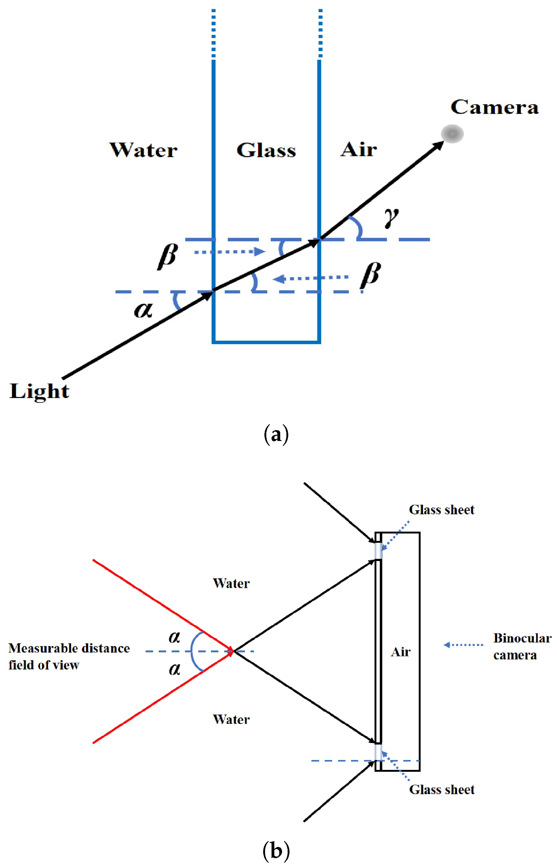
4.3. Analysis of Binocular Field of View

The underwater wide-angle system of the robot binocular system serves to detect the underwater environment, where we adopt waterproofing measurements on the shell.

Because of the light refraction, the large angle of the binocular camera observing the target underwater becomes smaller. Figure 5a shows the schematic light pattern from the maximum incident angle in the water to a given edge of a binocular camera. We assume that the wide angle of the camera is $\theta$, $\gamma =\frac{\theta }{2}$, the maximum incident angle of the water light to the waterproof glass foil is $\alpha$, the maximum refractive angle within the planar glass sheet is $\beta$ and thus, the maximum incident angle of the glass foil in the air is $\beta$ as well. It can be seen that the maximum refraction angle between the waterproof flat glass and the air where the camera is located is $\gamma$. The following Formula (11) can be obtained depending on the refracting law.

$$\begin{array}{c}\hfill n_{water}\times sin\alpha =n_{glass}\times sin\beta \\ \hfill n_{glass}\times sin\beta =n_{air}\times sin\gamma \end{array}$$

(11)

where $n_{water}$, $n_{glass}$ and $n_{air}$ represent the refraction index of the water media, glass media and air media, respectively. The formula can be translated into Formula (12),

$$sin\alpha =\frac{n_{air}}{n_{water}}\times sin\gamma$$

(12)

The air refractive index is about 1, whereas the water refractive index is 1.333. It can be calculated that the binocular camera used in this paper has a wide angle of 105 degrees, where $\gamma =52.5$ degrees. Therefore, $\alpha =36.5243$ degrees. The camera has a field of vision of about 73.0486 degrees. Figure 5b depicts the top view of the underwater visual field of the camera. Analysis in the binocular field of vision is linked to the feedback process for designing the vision-based formation system.

5. Multi-Robot Formation Control System Design

Usually, the multi-robot system is complemented by the interplay of information such as the kernel. Underwater communication is generally carried out through underwater acoustic communications. However, underwater acoustic communication differs from terrestrial wireless electromagnetic communication, which has a slow propagation speed, massive lag, instability, and energy consumption. Although many multi-robot formation algorithms exist in a good communication environment, it is challenging to train underwater multi-robots in practical applications in this weak communication condition.

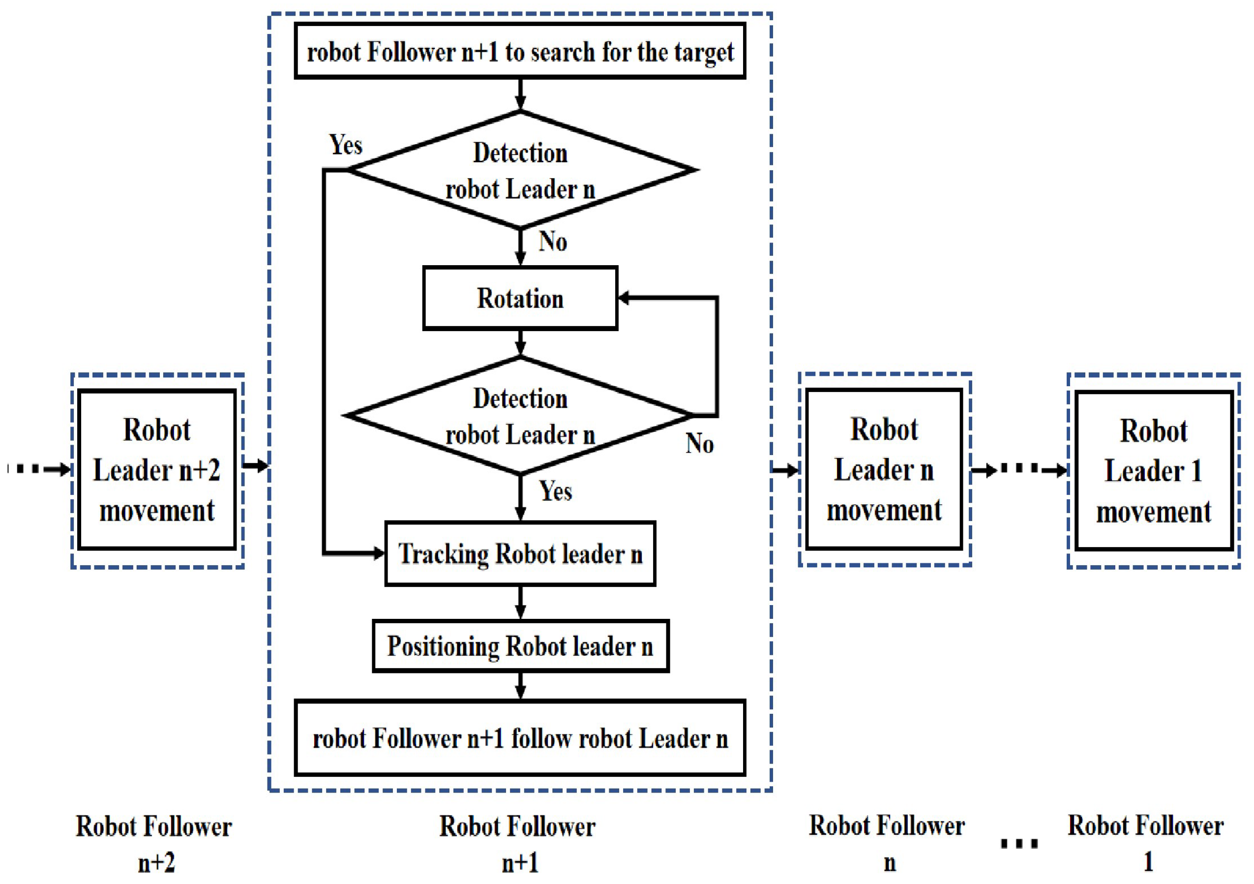
5.1. Formation Structure Design

In the case of robot training, most research is based on the exchange of information or simulation between robots. Not only is the algorithm complex, but because of the constraints of the underwater environment, it is not easy to communicate large-scale data in real time between robots wirelessly [58]. In this paper, we would like to solve the problem of formation difficulty in weak communication utilizing visual sensing, design the formation structure by using the series hierarchical formation system similar to the hierarchical structure, and use the leader-follower method to control the formation. Visual sensing means exchanging information through an optical system where the transmission can be achieved through the vision system without needing large-scale equipment [59]. Real-time communication realizes the regular operation of the formation of the robot by controlling the position information of the following robots and leaders.

Each robot is regarded as a rigid body in the underwater formation design of a small bionic spherical robot. Depending on the tasks involved, the size and shape of the robot training may be designed, which means the robot’s formation determines the robot’s distance and orientation in the formation.

The classic leader-follower formation control strategy is mainly used in two-dimensional planes [60]. More specifically, two methods are used to achieve formation control. One is an angle-distance feedback control method, and the other is a distance-distance feedback control method. The angle-distance-based feedback control method utilizes the deviation of the angle and distance between the follower robot and the leader robot to achieve the follower’s motion to maintain the queue. The distance-distance-based feedback control method uses the deviation of the distance between the follower and the two leader robots to achieve the follower’s movement to maintain the queue. The follower robot only needs to follow the leader, thus reducing resource allocation.

In this paper, we use a cascading approach to achieve the piloting of the robot to follow the formation. Each follower has a leader, and the entire multi-robot formation has only one leader. Figure 6 is the flow chart of the following actions the follower took in the formation. The overall process can be described as the robot follower n + 1 searching for the target and tracking the target’s movement through the visual system. The binocular positioning method is adopted to calculate the three-dimensional coordinate, which is the feedback of the motion control.

5.2. Modelling and Control of the Vision-Based Formation System

As this paper adopts a vision-based leader-follower formation control model, one pair of leader-follower formation control models can be used to study the model of the whole formation system control model.

To better present the scheme of the leader-follower, a kinematic equation is set up for a leader-follower pair, and a simple leader-follower configuration is displayed in Figure 7 [61,62].

$$\begin{array}{cc}& \dot{x}=vcos\theta \\ & \dot{z}=vsin\theta \\ & \dot{y}=v_y\\ & \dot{\theta }=\omega \end{array}$$

(13)

where $(x,y,z)$ represents the position of each robot, and $\theta$ is the orientation with respect to the world coordinate. v represents the velocity of the robot, and $\omega$ represents the angular velocity of the robot. The leader robot has a configuration vector ${\left[x_L{y}_L{z}_L{\theta }_L\right]}^T$, while the follower robot has a vector of ${\left[x_F{y}_F{z}_F{\theta }_F\right]}^T$.

Thus, the kinematic model of the leader robot and the follower robot can be obtained, which is similar to Equation (13). The control inputs of the follower are the declination distance and the declination course angle with respect to the leader, ${\mathit{u}}_F={\left[v_F{v}_{Fy}{\omega }_F\right]}^T$, respectively. $v_F$ represents the velocity on the XOZ plane of the follower. $v_{Fy}$ represents the velocity in the depth. ${\omega }_F$ represents the angular velocity of the course angle. The two-robot system is transformed into a new set of coordinates where the state of the leader is treated as an exogenous input. The outputs of the system are the position of the leader, for the moving process of the follower will inevitably cause the relative positioning change of the leader. The kinematic model can be written as follows:

$$\begin{array}{c}\dot{s}=G\left(s\right)u\end{array}$$

(14)

The kinematic model in the case of n followers can be obtained by extending Formula (13). In this case, the input vector can be rewritten as $\mathit{u}=[{\mathit{u}}_{\mathbf{1}}{\mathit{u}}_{\mathbf{2}}\dots {\mathit{u}}_{\mathit{n}}]$ and the state vector is $\mathit{s}={[{\mathit{s}}_{\mathbf{1}}^T\dots {\mathit{s}}_{\mathit{n}}^T]}^T$.

In particular, the three-dimensional positioning of the leader robot in its coordinate system is achieved by the follower robot’s vision system. Through the three-dimensional coordinates of the leader robot, various relative angles and distances of the follower robot and the leader robot are calculated. In the three-dimensional plane, offset feedback information enables the follower robot to follow the leader robot. Figure 8 shows the location information of the leader robot in the follower robot’s vision coordinate system.

The point P under the world system $O_w-X_w{Y}_w{Z}_w$ is $(X_w,Y_w,Z_w)$, which is also the center of the leader robot and the coordinate under the follower’s visual system $O_F-X_F{Y}_F{Z}_F$ is $(X_F,Y_F,Z_F)$, where the visual system is also the follower’s left camera coordinate and can be expressed as $O_{c1}-X_{c1}{Y}_{c1}{Z}_{c1}$, is $(X_{c1},Y_{c1},Z_{c1})$. According to that, the left camera coordinate is coincident with the world system, andthe point P under the left camera can be expressed as $(X_L,Y_L,Z_L)$, which is considered to be the center of the leader robot. Thus, the distance between the follower robot and the leader robot is $d_l=\sqrt{{d_s}^2+{d_y}^2}=\sqrt{{X_L}^2+{Y_L}^2+{Z_L}^2}$, where $d_x=\left|X_L\right|$, $d_y=\left|Y_L\right|$, $d_z=\left|Z_L\right|$, $d_s=\sqrt{{d_x}^2+{d_z}^2}=\sqrt{{X_L}^2+{Z_L}^2}$. The angle relationship between follower robot and the leader robot is $tan\theta =\frac{X_L}{Z_L}$, $tan\beta =\frac{Y_L}{\sqrt{{X_L}^2+{Z_L}^2}}$, $tan\alpha =\frac{\sqrt{{X_L}^2+{Y_L}^2}}{Z_L}$.

The control block diagram of the proposed algorithm for formation is as shown in Figure 9. In the three directions of the follower robot, its declination angle and offset with the leader robot are used. The PID control algorithm is used to realize the three-direction control, whose structure is similar to the structure shown in Figure 3. According to the diagram of the control system, the course control is implemented using the declination $\theta$ and the offset $d_x$. Depth control is achieved using declination $\beta$ and offset $d_y$. Velocity control is achieved using the bias moment $d_z$ and the offset distance $d_l$. The declination and offset of the leader robot with respect to the follower robot are $\alpha$ and $d_l$. Thus, the three controllers can be expressed as

$$\Delta {\omega }_F={\mathit{K}}_{\mathbf{1}}\Delta {\theta }_F$$

(15)

$$\Delta v_{Fy}={\mathit{K}}_{\mathbf{2}}\Delta Y_F$$

(16)

$$\Delta v_F={\mathit{K}}_{\mathbf{3}}\Delta Z_F$$

(17)

By substituting Equations (15)–(17) into Formulas (1) and (2), the control law can be obtained as Equations (18)–(20),

$$\begin{array}{cc}\hfill \Delta {\theta }_F\left(k\right)& =K_{p1}[\Delta {\omega }_F\left(k\right)-\Delta {\omega }_F(k-1)]+K_{i1}\Delta {\omega }_F\left(k\right)+K_{d1}[\Delta {\omega }_F\left(k\right)-2\Delta {\omega }_F(k-1)\hfill \\ \hfill & -\Delta {\omega }_F(k-2)]\hfill \end{array}$$

(18)

$$\begin{array}{cc}\hfill \Delta Y_F\left(k\right)& =K_{p2}[\Delta v_{Fy}\left(k\right)-\Delta v_{Fy}(k-1)]+K_{i2}\Delta v_{Fy}\left(k\right)+K_{d2}[\Delta v_{Fy}\left(k\right)-2\Delta v_{Fy}(k-1)\hfill \\ \hfill & -\Delta v_{Fy}(k-2)]\hfill \end{array}$$

(19)

$$\begin{array}{cc}\hfill \Delta Z_F\left(k\right)& =K_{p3}[\Delta v_F\left(k\right)-\Delta v_F(k-1)]+K_{i3}\Delta v_F\left(k\right)+K_{d3}[\Delta v_F\left(k\right)-2\Delta v_F(k-1)\hfill \\ \hfill & -\Delta v_F(k-2)]\hfill \end{array}$$

(20)

After determining the state information of the leader robot, the further problem to be studied is whether the error of the position and the angle converge to zero. If they converge to zero, it is proved that the following robot tracks the position of the leader robot in real-time. Because we use PID controllers, the whole system is stable when its open-loop transfer function is stable. In actual engineering practice, it is generally stable. Therefore, its stability will not be repeated in this paper. We reckoned that the whole system is sound.

Additionally, the declination angle between the leader robot and the follower robot’s binocular camera coordinate system along the Z-axis depends on the robots’ formation requirements because the direction of the force when the follower robot’s main course angle is the same as the direction of force when the leader robot is in the main course angle. When the follower robot is following the leader robot, each follower robot can maintain the following and the formation of the main robot by adjusting its course angle and speed so that the formation of the multi-robot system can be realized. Distance and orientation are provided by the vision system’s resolution information, and the leader robot is kept in a fixed position through the control of depth direction, course angle, and velocity. Therefore, the coordination period of the formation is determined by the visual system’s frame rate and the robot control frequency.

6. Experiments

6.1. Underwater Motion Control Experiment

In order to verify the stability and controllability of the new generation robot platform, we carried out a control experiment of a single robot in a laboratory pool, whose size is 3 m × 2 m × 1 m, with a water depth of about 0.5 m. The motion control experiment was divided into two small experiments. The first experiment was regarding the linear motion of the spherical robot, and the second experiment was on the rotation motion of the spherical robot. In the linear motion experiment, the real-time feedback of heading angle was used as the control quantity through the MENS sensor.

6.1.1. Linear Motion of a Single Robot

The spherical robot was controlled by the mentioned method. The heading angle was set as a fixed value of 71°. The robot started to move from the position where the heading angle was 0 until the robot makes a linear motion in the set fixed heading angle, as is shown in Figure 10. It can be concluded that the rise time for the linear movement control is about 8 s.

6.1.2. Rotation Motion of a Single Robot

To achieve the anti-loss mechanism in the formation system, the robot needed to be controlled to achieve the expected rotation movement. During the rotation motion control experiment, the water jet motors in the spherical robot’s left front and right rear were controlled to make the robot rotate with an approximate radius of 0, as shown in Figure 11.

6.2. Underwater Visual System Experiment

Underwater Camera Calibration Experiment

Camera calibration is the basis for visual system utilization, where the parameters of the camera to calculate the three-dimensional coordinates of the target can be obtained. The binocular camera parameters contain each camera’s intrinsic parameter matrix and the distortion coefficient matrix, the translation vector, and the rotation matrix for the two cameras. The whole calibration process is aimed at obtaining the internal and external parameters of camera 1 and camera 2.

This paper adopted the most widely used Zhengyou Zhang calibration method in the traditional camera calibration method [63,64]. The Zhengyou Zhang calibration method is easy to implement, has a simple calibration process, and is high in precision. To achieve accurate calibration of the binocular camera, this paper used the Matlab 2016 calibration toolbox for calibration. Firstly, the underwater images of the calibration board were simultaneously acquired by the left and right cameras of the binocular camera, where 103 pairs of images of the underwater calibration board were collected through the underwater camera calibration experiment. Figure 12a represents the physical status of one couple of pictures of the right camera and the left camera. Figure 12b shows the distribution of the calibrated board acquired. The overall mean error is 0.06 pixels. The results are listed in

Table 1. Results of underwater camera calibration experiment.

Parameters	Camera 1	Camera 2
Internal Matrix	$A_1={\left(\begin{array}{ccc}407.5947& 0& 0\\ 0.0471& 407.5793& 0\\ 162.1590& 115.1450& 1\end{array}\right)}^T$	$A_2={\left(\begin{array}{ccc}402.6531& 0& 0\\ 0.0764& 402.7510& 0\\ 161.8050& 118.4995& 1\end{array}\right)}^T$
Rotation Matrix	$R_1={\left(\begin{array}{ccc}1& 0& 0\\ 0& 1& 0\\ 0& 0& 1\end{array}\right)}^T$	$R_2={\left(\begin{array}{ccc}1.0000& 0.0017& -0.0041\\ -0.0016& 0.9996& 0.0279\\ 0.0042& -0.0279& 0.9996\end{array}\right)}^T$
Translation Vector	$T_1={\left(\begin{array}{ccc}1& 0& 0\end{array}\right)}^T$	$T_2={\left(\begin{array}{ccc}-62.0834& -0.3144& -0.2483\end{array}\right)}^T$

.

6.3. Underwater Formation Experiments

In order to further verify the effectiveness of the proposed method, this paper conducts experimental verification on a formation of two or three robots. Because of the limitation of the pool, there was one stable individual during the experiments with three robots. The formation experiment was abstracted from actual underwater formation missions, which has more significance for practical applications.

6.3.1. Underwater Vision-Based Ranging Experiment

In order to facilitate distance measurement, we used a yellow submarine model, which had a length of 10 cm, to perform real-time positioning and distance measurement. As shown in Figure 13, when distance measurement was performed, the recording of the scale distance was performed every 10 cm. Figure 14 shows the distance of the binocular camera’s measurement compared with the ruler. The root-mean-square error was used to measure the relationship between the distance measured by binocular camera vision and the distance measured by the ruler.

$$RMSE\left(d_z\right)=\sqrt{\frac{1}{n}{\displaystyle \sum _{i=1}^n}{(d_i-{\widehat{d}}_i)}^2}$$

(21)

where $d_i$ and ${\widehat{d}}_i$ are the distance between the object measured by the vision system and the ruler, respectively. The root-mean-square error in the underwater ranging experiment was 11.29 cm when the maximum of the distance was 160 cm. The approximate mean error rate was 7%. It can be concluded from Figure 13 that during the experiment of continuous positioning, the error mainly occurred in the return phase of distance from large to small. We speculate that the error may be caused by the change in the moving direction of the hand-held target as it left and returned, which produced ripples in different directions; the diffusion of such ripples brings optical interference. At the same time, it may also be because the target trembles during hand-held movement, which brings unexpected offset in the other directions. However, the magnitude of this error is acceptable. In the process of formation, we can reduce the impact of this error by building a closed-loop feedback regarding position.

6.3.2. Dynamic Straight-Line Formation Experiment

This experiment included two robots, where the leader was dynamic. The improved previous-generation underwater spherical robot was set as the leader robot, and the new-generation amphibious spherical robot was the follower robot. The leader robot performed a linear motion in a particular direction, and the follower robot navigated under the guidance of the leader robot to form the leader-follower formation structure.

Figure 15a–d show the status of the leader and follower robots captured on the global camera above the pool at 0 s, 5 s, 10 s and 15 s, respectively. Figure 16a–d show the state of the leader robot tracked by the binocular camera at 0 s, 5 s, 10 s and 15 s of the follower robot, respectively. In the process of linear motion, Figure 17a shows the course angle of the leader robot measured by the binocular vision system of the robot compared with the course angle change of the follower robot measured by the MENS sensor. Figure 17b shows the course angle transformation of the leader robot measured by the MENS sensor carried by the leader robot.

In Figure 17a, it can be seen that the leader robot’s course angle obtained by following the robot’s binocular vision system is near 90 degrees. That is, the leader robot was following the binocular vision system of the robot. In order to ensure that the leader robot is following the robot’s field of view, the follower robot adjusted itself. The course of the leader robot measured by the following robot is opposite to its course change trend, which ensures that the following robot keeps following the leader robot. The MENS measured data and the measured binocular data can represent the following robot’s heading angle and the leader’s heading angle, respectively. The opposite trend means that the heading angles of the two robots are gradually approaching the same, which also means that the positions of the two robots are getting closer.

Figure 18 shows the leader robot’s relative distance and relative three-dimensional coordinates on the respective coordinate axes measured by the binocular vision system of the follower robot in the formation process. As can be seen in Figure 18a, the distance between the follower robot and the leader robot in the Z-axis direction gradually becomes stable. Figure 19 is the frame rate of the follower robot vision system. During the whole movement, it can be seen that the frame rate of the binocular vision is stable at about 15 frames per second, which means it is feasible for application in actual underwater formation missions. It should be noted, though, that 15 frames per second is high, which may cause a lot of computational overhead. However, this visual frame rate will bring benefits that cannot be ignored in the visual feedback formation process. One of the necessary conditions for the proposed formation method of the leader-follower structure is that the follower can solve the relative position coordinates, which means that the follower must be able to detect and track the leader within its perspective. As shown in Figure 6, if the detection and tracking behavior fails, it will need to re-detect until the leader can be observed. If the visual frame rate is low when the leader’s speed is relatively high, it is easy for the leader to go out of the scene from the follower’s perspective, and the target may get lost, such that the formation process is easy to challenge. Therefore, even if the frame rate is 15 per second and the calculation cost is relatively higher than a lower frame rate, the increase in cost is still worthwhile.

6.3.3. “V-Type Escort” Formation Experiment

The “V-type escort” is rooted in cruiser escorts. In this experiment, the previous prototype was set as the first-level leader robot, which was in the stationary state, and the improved previous-generation underwater spherical robot, which was numbered No.2, and the new-generation amphibious spherical robot, which was numbered No.1, served as the follower robots. The following robots approached the leader robot at the same time, and the three robots maintained the “V-type” formation structure.

As shown in Figure 20a–d, the leader robot and the follower robots were captured by the global camera above the pool at 0 s, 3 s, 6 s and 9 s, respectively. Figure 21a–d show the state of the leader robot tracked by the binocular cameras on the No.1 follower robot at 0 s, 3 s, 6 s and 9 s, respectively. Figure 22a–d show the state of the leader robot tracked by the binocular cameras on the No. 2 follower robot at 0 s, 3 s, 6 s and 9 s, respectively.

Figure 23a shows the course angle of the leader robot measured by the No.1 follower robot vision system compared with its own heading angle measured by the MENS sensor. Figure 23b shows the course angle of the leader robot measured by the No.2 follower robot vision system compared with the own course angle measured by the MENS sensor. The MENS sensor itself is affected by the magnetic field and causes the data to suddenly change when t = 2 s, which is rooted in the susceptibility of the chosen JY901 IMU module. Compared with the six-axes IMU module, JY901 is a nine-axes module. It has three more magnetic field sensors in the three directions, which makes it more sensitive to changes in the magnetic field and makes it easy to generate magnetic interference.

As is shown in Figure 23b, it can be speculated that the water jet motor may cause some bad magnetic field during propulsion, which interferes with IMU data. Figure 24a,b are the distances measured by the No.1 follower robot and the No.2 follower robot through their vision systems, respectively. Figure 25a,b are the three-dimensional coordinates measured by the visual system of the No.1 follower robot and No.2 follower robot, respectively. Figure 26a,b are the frame rates of the No.1 follower robot and No.2 follower robot through their vision systems, respectively.

In the leader-follower formation, the No.1 follower robot moved to the leader robot. At the same time, the No.2 follower also moved to the leader robot, proving that two follower robots can maintain the “V-type” formation with the leader robot through this experiment.

6.3.4. “Round-Up Hunting” Formation Experiment

The “round-up hunting” formation is designed for the ideal underwater capture task, where small robots keep approaching the target and blocking its escape route. In this experiment, the previous generation prototype was set as the leader robot, which was static. In contrast, the new-generation amphibious spherical robot and the improved previous-generation underwater spherical robot served as follower robots. The follower robots approached the leader robot simultaneously, then encircled and caught the leader robot. The new-generation amphibious spherical robot was numbered as No.1, while the improved previous-generation underwater spherical robot was numbered as No.2.

As shown in Figure 27a–d, the state of the leader robot and follower robot was captured by the global camera above the pool at 0 s, 3 s, 6 s and 9 s, respectively. Figure 28a–d show the state of the leader robot tracked by the binocular cameras on the No.1 follower robot at 0 s, 3 s, 6 s and 9 s, respectively. Figure 29a–d show the state of the leader robot tracked by the binocular cameras on the No.2 follower robot at 0 s, 3 s, 6 s and 9 s, respectively.

Figure 30a shows the course angle of the leader robot measured by the No.1 follower robot vision system compared with its course angle measured by the MENS sensor. Figure 30b shows the course angle of the leader robot measured by the No.2 follower robot vision system compared with its course angle measured by the MENS sensor. Figure 31a,b are the measured distances of the No.1 follower robot and No.2 follower robot, respectively. Figure 32a,b are the three-dimensional coordinates measured by the vision system of the No.1 follower robot and the No.2 follower robot, respectively. Figure 33a,b are the frame rates of the No.1 follower robot and No.2 follower robot, respectively. In the leader-follower formation, the No.1 follower robot moves to the leader robot. In contrast, the No.2 follower robot moves to the leader robot simultaneously, proving that two follower robots can “round up” the leader robot at the same time through this experiment.

7. Discussion

Because this paper adopts a cascade leader-follower structure to follow the formation strategy, it is necessary to study a pair of leader-follower robot systems to achieve the formation of multiple robots.

Two factors mainly cause the error of the underwater robot formation system: one is the robot motion control precision, and the other is the binocular vision system of the robot. The accuracy of motion control is generally accomplished by adjusting the frequency of control movement and the parameters of PID controllers. In the formation experiment, the time interval of motion adjustment is about 50 ms. The errors caused by binocular vision systems mainly come from two aspects: the error of binocular measurement and the frame rate of the binocular system. The frame rate of the binocular system is about 15FPS. In particular, we have to mention that the visual frame rate and control frequency are closely related to hardware conditions, and both need to consider the computational cost and overhead of the whole system. Theoretically, increasing the control frequency and frame rate will reduce the error, but from the perspective of robot manufacturing, this improvement is limited, especially in the design of small underwater robots, where there are multiple restrictions on the selection of hardware, which may bring restrictions on computing capacity, power, battery capacity, and so on.

The measurement error of the binocular system is mainly rooted in the camera calibration and the camera shaking during the tracking process. It can be concluded from the underwater ranging experiment that the mean error is mostly 11 cm when the maximum distance is 160 cm, with an approximate mean error rate of 7%.

Due to the particularity of the underwater environment compared with the terrestrial environment, its light transmittance is poor, its image is easy to twist and deform, and the transparency of the water body and the plankton content will affect binocular measurements. However, this effect is relatively slight under short distance conditions, such as the range under the laboratory conditions. In practical application, once the distance between two underwater robots is too far, the visual measurement effect will be significantly reduced, such that the long distance not only declines the image quality but also affect the similar triangles set up during binocular ranging, where the two sides of the triangle can be reckoned as approximately parallel when the target is too far.

In addition, we have noticed that in other people’s work, without using additional markers such as lasers, the maximum distance to complete underwater visual relative positioning is beyond 3 m [65,66]. Therefore, in practical application, without the aid of other auxiliary optical equipment, it is acceptable to study the formation of centimeter-level positioning and complete visual feedback. In this paper, we can achieve 20 cm to 200 cm ranging and positioning by utilizing the binocular system in the laboratory pool environment. We can also theoretically achieve underwater formations in the range of 200 cm.

Additionally, the current time scale of the experiment is about 20 s, and the time should be expanded to understand how it works over a long distance. Frankly speaking, compared with large-scale underwater robots, small-scale underwater robots generally work for less than one hour due to the limitations of their power supplies. At the same time, due to the particularity of formation tasks, potential obstacles cannot be ignored when moving long distances. Therefore, the proposed visual feedback leader-follower formation may be challenged in long-term and long-distance formation practical tasks. These challenges may come from potential movable obstacles or the MENS module’s cumulative error. However, the MENS sensor JY901 chosen in this paper has high accuracy and a built-in filter module, so the accumulated error in long-time use is smaller than other ordinary sensors. Therefore, it is feasible for general time formation tasks.

8. Conclusions

In this paper, a vision-based formation control method based on the leader-follower structure is designed. The visual system is set as the consensus means for positioning and measurement, where the field of view on the binocular camera is analyzed, and the visual solution quantities are calculated and set as the input of the formation control system to achieve the vision-based formation control. The control diagram of the formation control system and the control law is discussed. Meanwhile, underwater formation experiments, including the “Dynamic Straight-line” formation experiment, “V-type Escort,” and “Round-up Hunting,” which are abstracted from actual underwater missions, are implemented. Furthermore, the coordinate time as well as the error of the formation system, is analyzed. The error of the underwater robot formation system is mainly caused by the robot motion control precision, evaluated during the motion control experiments, and error measured by the binocular vision system, which the vision-based ranging experiment has discussed. Additionally, the long-time effect of the formation is discussed to demonstrate the proposed method’s effectiveness and practicability.

References

1. Yuh, J.; West, M. Underwater robotics. Adv. Robot. 2001, 15, 609–639. [Google Scholar] [CrossRef]
2. Sivčev, S.; Coleman, J.; Omerdić, E.; Dooly, G.; Toal, D. Underwater manipulators: A review. Ocean. Eng. 2018, 163, 431–450. [Google Scholar] [CrossRef]
3. Sahoo, A.; Dwivedy, S.; Robi, P. Advancements in the field of autonomous underwater vehicle. Ocean. Eng. 2019, 181, 145–160. [Google Scholar] [CrossRef]
4. Wu, Y.; Low, K.H.; Lv, C. Cooperative path planning for heterogeneous unmanned vehicles in a search-and-track mission aiming at an underwater target. IEEE Trans. Veh. Technol. 2020, 69, 6782–6787. [Google Scholar] [CrossRef]
5. Saback, R.; Conceicao, A.; Santos, T.; Albiez, J.; Reis, M. Nonlinear model predictive control applied to an autonomous underwater vehicle. IEEE J. Ocean. Eng. 2020, 45, 799–812. [Google Scholar] [CrossRef]
6. Zhou, Z.; Liu, J.; Yu, J. A survey of underwater multi-robot systems. IEEE/CAA J. Autom. Sin. 2021, 1, 1–18. [Google Scholar] [CrossRef]
7. Connor, J.; Champion, B.; Joordens, M.A. Current algorithms, communication methods and designs for underwater swarm robotics: A review. IEEE Sens. J. 2020, 1, 153–169. [Google Scholar] [CrossRef]
8. Chen, W.; Zhang, Y.; Wen, J.; Li, K.; Yang, G. An Application of Improved RANSAC Algorithm in Visual Positioning. In Proceedings of the 2019 IEEE 8th Joint International Information Technology and Artificial Intelligence Conference (ITAIC), Chongqing, China, 24–26 May 2019; pp. 1358–1362. [Google Scholar] [CrossRef]
9. Cui, R.X.; Ge, S.Z.S.; How, B.V.E.; Choo, Y.S. Leader-follower formation control of underactuated autonomous underwater vehicles. Ocean. Eng. 2010, 37, 1491–1502. [Google Scholar] [CrossRef]
10. Wang, J.Q.; Wang, C.; Wei, Y.J.; Zhang, C.J. Sliding mode based neural adaptive formation control of underactuated AUVs with leader-follower strategy. Appl. Ocean. Res. 2020, 94, 101971. [Google Scholar] [CrossRef]
11. Makavita, C.; Jayasinghe, S.; Nguyen, H.; Ranmuthugala, D. Experimental study of command governor adaptive control for unmanned underwater vehicles. IEEE Trans. Control Syst. Technol. 2019, 27, 332–345. [Google Scholar] [CrossRef]
12. Beard, R.W.; Lawton, J.; Hadaegh, F.Y. A coordination architecture for spacecraft formation control. IEEE Trans. Control Syst. Technol. 2001, 9, 777–790. [Google Scholar] [CrossRef]
13. Fiorelli, E.; Leonard, N.E.; Bhatta, P.; Paley, D.A.; Bachmayer, R.; Fratantoni, D.M. Multi-AUV control and adaptive sampling in Monterey Bay. IEEE J. Ocean. Eng. 2006, 31, 935–948. [Google Scholar] [CrossRef]
14. An, R.; Guo, S.; Yu, Y.; Li, C.; Awa, T. Task Planning and Collaboration of Jellyfish-inspired Multiple Spherical Underwater Robots. J. Bionic Eng. 2022, 3, 643–656. [Google Scholar] [CrossRef]
15. Balch, T.; Arkin, R.C. Behavior-based formation control for multirobot teams. IEEE Trans. Robot. Autom. 1998, 14, 926–939. [Google Scholar] [CrossRef]
16. dell’Erba, R. Swarm robotics and complex behaviour of continuum material. Contin. Mech. Thermodyn. 2019, 31, 989–1014. [Google Scholar] [CrossRef]
17. Hadi, B.; Khosravi, A.; Sarhadi, P. A review of the path planning and formation control for multiple autonomous underwater vehicles. J. Intell. Robot. Syst. 2021, 101, 67. [Google Scholar] [CrossRef]
18. Shojaei, K.; Chatraei, A. Robust platoon control of underactuated autonomous underwater vehicles subjected to nonlinearities, uncertainties and range and angle constraints. Appl. Ocean. Res. 2021, 110, 102594. [Google Scholar] [CrossRef]
19. Chen, Y.L.; Ma, X.W.; Bai, G.Q.; Sha, Y.; Liu, J. Multi-autonomous underwater vehicle formation control and cluster search using a fusion control strategy at complex underwater environment. Ocean. Eng. 2020, 216, 108048. [Google Scholar] [CrossRef]
20. Liu, H.; Wang, Y.; Lewis, F.L. Robust Distributed Formation Controller Design for a Group of Unmanned Underwater Vehicles. IEEE Trans. Syst. Man Cybern. Syst. 2019, 51, 1215–1223. [Google Scholar] [CrossRef]
21. Gao, Z.; Guo, G. Velocity free leader-follower formation control for autonomous underwater vehicles with line-of-sight range and angle constraints. Inf. Sci. 2019, 486, 359–378. [Google Scholar] [CrossRef]
22. Liang, H.; Fu, Y.; Gao, J.; Cao, H. Finite-time velocity-observed based adaptive output-feedback trajectory tracking formation control for underactuated unmanned underwater vehicles with prescribed transient performance. Ocean. Eng. 2021, 233, 109071. [Google Scholar] [CrossRef]
23. Xiang, X.; Jouvencel, B.; Parodi, O. Coordinated formation control of multiple autonomous underwater vehicles for pipeline inspection. Int. J. Adv. Robot. Syst. 2010, 1, 3. [Google Scholar] [CrossRef]
24. Cao, X.; Guo, L. A leader–follower formation control approach for target hunting by multiple autonomous underwater vehicle in three-dimensional underwater environments. Int. J. Adv. Robot. Syst. 2019, 4, 1729881419870664. [Google Scholar] [CrossRef]
25. He, S.; Wang, M.; Dai, S.L.; Luo, F. Leader–follower formation control of USVs with prescribed performance and collision avoidance. IEEE Trans. Ind. Inform. 2018, 15, 572–581. [Google Scholar] [CrossRef]
26. Lin, J.; Miao, Z.; Zhong, H.; Peng, W.; Wang, Y.; Fierro, R. Adaptive image-based leader–follower formation control of mobile robots with visibility constraints. IEEE Trans. Ind. Electron. 2020, 68, 6010–6019. [Google Scholar] [CrossRef]
27. Han, Z.; Guo, K.; Xie, L.; Lin, Z. Integrated relative localization and leader–follower formation control. IEEE Trans. Autom. Control 2018, 64, 20–34. [Google Scholar] [CrossRef]
28. Gao, Z.; Guo, G. Fixed-time leader-follower formation control of autonomous underwater vehicles with event-triggered intermittent communications. IEEE Access 2018, 6, 27902–27911. [Google Scholar] [CrossRef]
29. Ai, X.; Yu, J. Flatness-based finite-time leader–follower formation control of multiple quadrotors with external disturbances. Aerosp. Sci. Technol. 2019, 92, 20–33. [Google Scholar] [CrossRef]
30. Zhang, Z.; Yang, T.; Zhang, T.; Zhou, F.; Cen, N.; Li, T.; Xie, G. Global vision-based formation control of soft robotic fish swarm. Soft Robotics 2021, 3, 310–318. [Google Scholar] [CrossRef]
31. Zheng, L.; Guo, S.; Piao, Y.; Gu, S.; An, R. Collaboration and Task Planning of Turtle-Inspired Multiple Amphibious Spherical Robots. Micromachines 2020, 11, 71. [Google Scholar] [CrossRef]
32. He, Y.; Zhu, L.; Sun, G.; Dong, M. Study on formation control system for underwater spherical multi-robot. Microsyst. Technol. 2019, 4, 1455–1466. [Google Scholar] [CrossRef]
33. Campos, R.; Gracias, N.; Ridao, P. Underwater multi-vehicle trajectory alignment and mapping using acoustic and optical constraints. Sensors 2016, 3, 387. [Google Scholar] [CrossRef] [PubMed]
34. Millán, P.; Orihuela, L.; Jurado, I.; Rubio, F.R. Formation control of autonomous underwater vehicles subject to communication delays. IEEE Trans. Control Syst. Technol. 2013, 2, 770–777. [Google Scholar] [CrossRef]
35. Das, B.; Subudhi, B.; Pati, B.B. Adaptive sliding mode formation control of multiple underwater robots. Arch. Control Sci. 2014, 4, 515–543. [Google Scholar] [CrossRef]
36. Qi, X.; Cai, Z. Three-dimensional formation control based on nonlinear small gain method for multiple underactuated underwater vehicles. Ocean. Eng. 2018, 4, 515–543. [Google Scholar] [CrossRef]
37. Fukuda, T. Cyborg and Bionic Systems: Signposting the Future. Cyborg Bionic Syst. 2020, 2020, 1310389. [Google Scholar] [CrossRef]
38. Shi, Q.; Gao, J.; Wang, S.; Quan, X.; Jia, G.; Huang, Q.; Fukuda, T. Deveopment of a Small-Sized Quadruped Robotic Rat Capable of Multimodal Motions. IEEE Trans. Robot. 2022, 1–17. [Google Scholar] [CrossRef]
39. Shi, Q.; Gao, Z.; Jia, G.; Li, C.; Huang, Q.; Ishii, H.; Takanishi, A.; Fukuda, T. Implementing Rat-Like Motion for a Small-Sized Biomimetic Robot Based on Extraction of Key Movement Joints. IEEE Trans. Robot. 2021, 3, 747–762. [Google Scholar] [CrossRef]
40. Namiki, A.; Yokosawa, S. Origami folding by multifingered hands with motion primitives. Cyborg Bionic Syst. 2021, 2021, 9851834. [Google Scholar] [CrossRef]
41. Wang, Y.; Li, W.; Togo, S.; Yokoi, H.; Jiang, Y. Survey on Main Drive Methods Used in Humanoid Robotic Upper Limbs. Cyborg Bionic Syst. 2021, 2021, 9817487. [Google Scholar] [CrossRef]
42. Shi, L.; Bao, P.; Guo, S.; Chen, Z.; Zhang, Z. Underwater Formation System Design and Implement for Small Spherical Robots. IEEE Syst. J. 2022. [Google Scholar] [CrossRef]
43. Lin, X.; Guo, S. Development of a spherical underwater robot equipped with multiple vectored water-jet-based thrusters. J. Intell. Robot. Syst. 2012, 3, 307–321. [Google Scholar] [CrossRef]
44. Xing, H.; Shi, L.; Hou, X.; Liu, Y.; Hu, Y.; Xia, D.; Li, Z.; Guo, S. Design, modeling and control of a miniature bio-inspired amphibious spherical robot. Mechatronics 2021, 77, 102574. [Google Scholar] [CrossRef]
45. Shi, L.; Hu, Y.; Su, S.; Guo, S.; Xing, H.; Hou, X.; Liu, Y.; Chen, Z.; Li, Z.; Xia, D. A fuzzy PID algorithm for a novel miniature spherical robots with three-dimensional underwater motion control. J. Bionic Eng. 2020, 5, 959–969. [Google Scholar] [CrossRef]
46. Xing, H.; Guo, S.; Shi, L.; Hou, X.; Liu, Y.; Liu, H. Design, modeling and experimental evaluation of a legged, multi-vectored water-jet composite driving mechanism for an amphibious spherical robot. Microsyst. Technol. 2020, 2, 475–487. [Google Scholar] [CrossRef]
47. He, Y.; Guo, S.; Shi, L.; Xing, H.; Chen, Z.; Su, S. Motion characteristic evaluation of an amphibious spherical robot. Int. J. Robot. Autom. 2019, 3. [Google Scholar] [CrossRef]
48. Guo, S.; He, Y.; Shi, L.; Pan, S.; Xiao, R.; Tang, K.; Guo, P. Modeling and experimental evaluation of an improved amphibious robot with compact structure. Robot. Comput.-Integr. Manuf. 2018, 51, 37–52. [Google Scholar] [CrossRef]
49. He, Y.; Zhu, L.; Sun, G.; Qiao, J.; Guo, S. Underwater motion characteristics evaluation of multi amphibious spherical robots. Microsyst. Technol. 2019, 2, 499–508. [Google Scholar] [CrossRef]
50. Xing, H.; Guo, S.; Shi, L.; He, Y.; Su, S.; Chen, Z.; Hou, X. Hybrid locomotion evaluation for a novel amphibious spherical robot. Appl. Sci. 2018, 2, 156. [Google Scholar] [CrossRef] [Green Version]
51. Li, Y.; Guo, S.; Yue, C. Preliminary concept of a novel spherical underwater robot. Int. J. Mechatron. Autom. 2015, 1, 11–21. [Google Scholar] [CrossRef]
52. Xing, H.; Liu, Y.; Guo, S.; Shi, L.; Hou, X.; Liu, W.; Zhao, Y. A Multi-Sensor Fusion Self-Localization System of a Miniature Underwater Robot in Structured and GPS-Denied Environments. IEEE Sens. J. 2021, 23, 27136–27146. [Google Scholar] [CrossRef]
53. Shi, L.; Guo, S.; Mao, S.; Yue, C.; Li, M.; Asaka, K. Development of an amphibious turtle-inspired spherical mother robot. J. Bionic Eng. 2013, 4, 446–455. [Google Scholar] [CrossRef]
54. Li, M.; Guo, S.; Hirata, H.; Ishihara, H. Design and performance evaluation of an amphibious spherical robot. Robot. Auton. Syst. 2015, 64, 21–34. [Google Scholar] [CrossRef]
55. Hou, X.; Guo, S.; Shi, L.; Xing, H.; Liu, Y.; Liu, H.; Hu, Y.; Xia, D.; Li, Z. Hydrodynamic analysis-based modeling and experimental verification of a new water-jet thruster for an amphibious spherical robo. Sensors 2019, 19, 259. [Google Scholar] [CrossRef] [PubMed]
56. dell’Erba, R. Distance estimations in unknown sea underwater conditions by power LED for robotics swarms. Contin. Mech. Thermodyn. 2021, 33, 97–106. [Google Scholar] [CrossRef]
57. dell’Erba, R. The distances measurement problem for an underwater robotic swarm: A semi-experimental trial, using power LEDs, in unknown sea water conditions. Contin. Mech. Thermodyn. 2020, 2020, 1–9. [Google Scholar] [CrossRef]
58. Suryendu, C.; Subudhi, B. Formation control of multiple autonomous underwater vehicles under communication delays. IEEE Trans. Circuits Syst. II Express Briefs 2020, 12, 3182–3186. [Google Scholar] [CrossRef]
59. Wu, Y.; Ta, X.; Xiao, R.; Wei, Y.; An, D.; Li, D. Survey of underwater robot positioning navigation. Appl. Ocean. Res. 2019, 90, 101845. [Google Scholar] [CrossRef]
60. Desai, J.P.; Ostrowski, J.; Kumar, V. Controlling formations of multiple mobile robots. In Proceedings of the 1998 IEEE International Conference on Robotics and Automation (Cat. No.98CH36146), Leuven, Belgium, 20–20 May 1998. [Google Scholar]
61. Das, A.K.; Fierro, R.; Kumar, V.; Ostrowsky, J.P.; Spletzer, J.; Taylor, C. A vision-based formation control framework. IEEE Trans. Robot. Autom. 2002, 5, 813–825. [Google Scholar] [CrossRef] [Green Version]
62. Mariottini, G.L.; Pappas, G.; Prattichizzo, D.; Daniilidis, K. Vision-based localization of leader-follower formations. In Proceedings of the 44th IEEE Conference on Decision and Control, Seville, Spain, 15 December 2005; pp. 635–640. [Google Scholar]
63. Zhang, Z. A flexible new technique for camera calibration. IEEE Trans. Pattern Anal. Mach. Intell. 2000, 11, 1330–1334. [Google Scholar] [CrossRef] [Green Version]
64. Heikkila, J.; Silven, O. Controlling formations of multiple mobile robots. In Proceedings of the 1997 IEEE Computer Society Conference on Computer Vision and Pattern Recognition, Santa Barbara, CA, USA, 23–25 June 1998. [Google Scholar]
65. Zheng, B.; Zheng, H.; Zhao, L.; Gu, Y.; Sun, L.; Sun, Y. Underwater 3D target positioning by inhomogeneous illumination based on binocular stereo vision. In Proceedings of the IEEE 2012 Oceans-Yeosu, Yeosu, Korea, 21–24 May 2012; pp. 1–4. [Google Scholar]
66. Tu, D.; Xu, Z.; Liu, C. The Influence of Active Projection Speckle Patterns on Underwater 3d Measurement Based on Binocular Stereo Vision. 2022. Available online: http://dx.doi.org/10.2139/ssrn.4107116 (accessed on 21 September 2022).
Figure 1. The overall structural design and the improved motor jet of the underwater spherical robot platform [50,55].
Machines 10 00877 g001
Figure 2. Electrical devices and modules of the new-generation spherical robot platform.
Machines 10 00877 g002
Figure 3. The block diagram of the heading angle control during a single robot motion.
Machines 10 00877 g003
Figure 4. Imaging schematic diagram of binocular camera.
Machines 10 00877 g004
Figure 5. The diagram of refraction phenomenon on the binocular camera. (a) The diagram of the maximum incident angle to a certain edge. (b) The top view of the camera’s underwater visual field.
Machines 10 00877 g005
Figure 6. The flow chart of the actions taken by the follower.
Machines 10 00877 g006
Figure 7. The schematic diagram of the formation movements taken by a pair of leader-follower robot systems.
Machines 10 00877 g007
Figure 8. The schematic diagram of visual solution information feedback.
Machines 10 00877 g008
Figure 9. The control diagram of the leader-follower formation system based on vision feedback.
Machines 10 00877 g009
Figure 10. Results of the linear motion experiment of a single robot.
Machines 10 00877 g010
Figure 11. Results of the rotation motion experiment of a single robot.
Machines 10 00877 g011
Figure 12. The calibration experiment of a binocular camera. (a) The physical status of one pair of images. (b) The distribution of the calibrated pairs of images.
Machines 10 00877 g012
Figure 13. The scheme of the underwater Vision-based ranging experiment where the yellow submarine model moved 10 cm each stage.
Machines 10 00877 g013
Figure 14. The distance on the Z-axis measured by the binocular camera compared with the ruler.
Machines 10 00877 g014
Figure 15. Images of global perspective and follower perspective of two robots dynamic straight-line formation experiment.
Machines 10 00877 g015
Figure 16. Images of follower perspective of two robots in a dynamic straight-line formation experiment.
Machines 10 00877 g016
Figure 17. The course angle measured by the vision of the follower robot and the leader robot compared with the self course angle measured by the MENS sensor over time.
Machines 10 00877 g017
Figure 18. Distance measured by the follower robot’s vision system.
Machines 10 00877 g018
Figure 19. Frame rate measured by the vision of the follower robot over time.
Machines 10 00877 g019
Figure 20. Images of global perspective and follower perspective of the three-robot “V-type escort” formation experiment.
Machines 10 00877 g020
Figure 21. Images of first-level follower perspective and follower perspective of the three-robot “V-type escort” following formation experiment.
Machines 10 00877 g021
Figure 22. Images of second-level follower perspective and follower perspective of the three-robot “V-type escort” following formation experiment.
Machines 10 00877 g022
Figure 23. The yaw angle measured by the vision of first-level follower robot and the second-level follower robot compared with the self yaw angle measured by the MENS sensor over time.
Machines 10 00877 g023
Figure 24. Distance measured by the first-level follower robot and the second-level follower robot over time.
Machines 10 00877 g024
Figure 25. Three-dimensional coordinates measured by the vision of the first-level follower robot and the second-level follower robot over time.
Machines 10 00877 g025
Figure 26. Frame rate measured by the vision of the first-level follower robot and the second-level follower robot over time.
Machines 10 00877 g026
Figure 27. Images of global perspective and follower perspective of the three-robot “round-up hunting” formation experiment.
Machines 10 00877 g027
Figure 28. Images of First-level follower perspective and follower perspective of the three-robot “round-up hunting” formation experiment.
Machines 10 00877 g028
Figure 29. Images of second-level follower perspective and follower perspective of the three-robot “Round-up hunting” formation experiment.
Machines 10 00877 g029
Figure 30. The yaw angle measured by the vision of first-level follower robot and the second-level follower robot compared with the self yaw angle measured by the MENS sensor over time.
Machines 10 00877 g030
Figure 31. Distance measured by the first-level follower robot and the second-level follower robot over time.
Machines 10 00877 g031
Figure 32. Three-dimensional coordinates measured by the vision of the first-level follower robot and the second-level follower robot over time.
Machines 10 00877 g032
Figure 33. Frame rate measured by the vision of the first-level follower robot and the second-level follower robot over time.
Machines 10 00877 g033