Multi-Layered Graph Convolutional Network-Based Industrial Fault Diagnosis with Multiple Relation Characterization Capability

Abstract

Fault diagnosis of industrial equipments is extremely important for the safety requirements of modern production processes. Lately, deep learning (DL) has been the mainstream fault diagnosis tool due to its powerful representational ability in learning and flexibility. However, most of the existing DL-based methods may suffer from two drawbacks: Firstly, only one metric is used to construct networks, thus multiple kinds of potential relationships between nodes are not explored. Secondly, there are few studies on how to obtain better node embedding by aggregating the features of different neighbors. To compensate for these deficiencies, an advantageous intelligent diagnosis scheme termed AE-MSGCN is proposed, which employs graph convolutional networks (GCNs) on multi-layer networks in an innovative manner. In detail, AE is carried out to extract deep representation features in process measurement and then combined with different metrics (i.e., K-nearest neighbors, cosine similarity, path graph) to construct the multi-layer networks for better multiple interaction characterization among nodes. After that, intra-layer convolutional and inter-layer convolutional methods are adopted for aggregating extensive neighbouring information to enrich the representation of nodes and diagnosis performance. Finally, a benchmark platform and a real-world case both verify that the proposed AE-MSGCN is more effective and practical than the existing state-of-the-art methods.

1. Introduction

With the development of information technology and the wide use of intelligent instruments, industrial machines are gradually presenting the characteristics of integration and complexity. Therefore, intelligent diagnosis of equipment fault is of great significance to the stable operation of equipment, the improvement of production efficiency and the increase of economic benefits [1,2,3]. Among the existing fault diagnosis approaches, the model-based class is considered to be the earliest and most widely used technique. The core idea of model-based ones is to construct a physical model or a state observer to realize fault diagnosis. However, prior knowledge of complex industrial equipment is not always available, which may limit the availability of model-based diagnosis methods.

Parallel to model-based ones, the data-based class has also been studied extensively due to its simplicity in diagnosing machine faults [4]. In addition, with the improvement of data collection and storage capabilities, the development of data-based methods is further promoted. For example, Zhong et al. [5] designed a principal component analysis (PCA)-based advantageously distributed scheme for fault diagnosis of a large-scale marine diesel engine. Recently, aiming at the shortcomings of the canonical correlation analysis (CCA) model, the authors of [6] proposed an SsCCA method and verified it with a nonlinear three-tank system. Lu and Yan [7] combined the Fisher discriminant analysis (FDA) and extreme learning machines (ELMs) to classify the fault feature vectors and shown advantages in visual industrial process diagnosis. Jiang et al. [8] presented latent variable correlation analysis (LVCA), which considered the correlation within units and between units simultaneously and achieved desired monitoring and diagnosis performance in large-scale plant-wide industrial processes. In [9], Garcia et al. used independent component analysis (ICA) to find the substantial differences between faulty and healthy motors. After that, Zhou et al. [10] integrated the PCA and ICA to comprehensively diagnose the abnormal furnace conditions of blast furnace (BF) ironmaking. Although these methods have shown some advantages, they are essentially shallow models, which may set up barriers for the applications of these methods in industrial big data scenarios.

In recent years, there has been rapid improvement in graphics processing unit (GPU) computing power and the accumulation of running data. Tremendous deep learning (DL) schemes have been proposed with extensive applications in face recognition [11], image classification [12] and process monitoring [13]. Inspired by the above studies, DL approaches have been gradually addressed by scholars in the fault diagnosis community and great successes have ben achieved. Concretely, Yang et al. designed [14] a lightweight convolutional neural network (CNN) model and demonstrated absolute advantages over the state-of-the-art methods. Gao et al. [15] presented a self-adaptive deep belief network (DBN), which improved the classification accuracy of the conventional DBN model significantly. The autoencoder (AE) [16] emphasized the depth of the model structure, reconstructed the original input through the structure of the encoder and decoder, and finally formed a more abstract feature vector suitable for classification, thereby improving the accuracy of fault diagnosis. Thus, the authors of [17] proposed a new multi-sensor data fusion technology, which sent the extracted features into a multiple two-layer sparse auto-encoder (SAE) for feature fusion, and the fused feature vectors can be used as machine health state diagnosis and classification. Yuan et al. [18] realized the fault prediction of boiling points in the industrial hydrocracking process by the spatiotemporal attention-based long short-term memory (LSTM) network, which can locate the key variables.

However, the above-mentioned DL-based models are only applicable to the regular grid data, ignoring the topology structure and the interactions of process variables. In this context, graph neural networks (GNNs) were proposed to process data characterized by complex spatiotemporal relationships, and non-Euclidean representations were exploited [19], and have been successfully applied in various domains [20,21], such as chemistry [22], commonsense reasoning [23], natural-language processing [24], social networks [25] and traffic flow prediction [26]. For example, the authors of reference [27] proposed a multi-scale graph node attention convolutional network diagnosis method. First, an adjacency matrix was set up according to the Pearson metric unsupervised convolutional auto-encoder, and then different neighbors on different nodes were evaluated. Chen et al. [28] fused the structural analysis (SA) and graph convolutional network (GCN) and achieved better diagnosis results regarding the traction system rectifier circuit. Then, Li et al. [29] incorporated the weighted horizontal visibility graph (WHVG) into the GCN model, which showed enhanced fault diagnosis performance with respect to real-world bearing compared with LSTM and general GCN models. Recently, since most of the existing methods ignore the distribution discrepancy of the data in different domains, the authors of [30] carried out a domain adversarial graph convolutional network to solve the above dilemma.

Although various approaches have been successfully applied for fault diagnosis, there are still some common problems in the previous studies: First, all existing state-of-the-art models only build a single-layer network for the original measured data; thus, the potential relationships between nodes are described through only one metric. However, in the real-world fault diagnosis task, signal samples can often interact in many different ways, e.g., there are multiple types of interactions simultaneously among samples [31,32]. Various potential relationships between nodes correspond to different neighbor information. By aggregating the information of different types of neighbors, better node features can be learnt, which are neglected by the single-layer network model. Additionally, though GCN layers are able to work with graphs, they cannot be used to process multi-layer networks directly and, considering their importance and ubiquity, further works are needed to overcome this difficulty.

Although some studies have addressed the topic of multi-layer GCN and AE, the work in this paper is different from them. More precisely, AE is used to constrain the hidden layers in [33,34], but not for the deep feature extraction. In [35], the framework of multilayer networks and the downstream tasks are both different from that in this paper. Motivated by the above research status and inspired by the GCN model, this paper constructs a multi-layer network through various metrics, and proposes an AE-based multi-layer structured GCN (AE-MSGCN) to obtain more robust node features for follow-up fault diagnosis. The main contributions of this work are summarized as follows:

(1)

Given that the complex and diverse relationships between process measurements, diversified multi-layer networks are constructed through three different metrics (i.e., Euclidean distance, cosine similarity, and path graph). Thus, the potential relationships among samples can be better characterized.

(2)

Different GCN layers are utilized to propagate the node features simultaneously and independently. Then, for each node, its representation in different layers is aggregated by multi-layer networks, which is beneficial for the enhancement of diagnostic performance.

(3)

Experiments are performed on both the simulated and real-word datasets and verify that the proposed AE-MSGCN scheme has better robustness and higher diagnostic accuracy than that of the state-of-the-art GCN-based fault diagnosis approaches.

The remainder of this paper is organized as follows. Section 2 gives the necessary preliminaries. The proposed AE-MSGCN method is introduced in Section 3. Section 4 are the simulation results and analyses. Finally, Section 5 summarizes the paper.

2. Preliminaries

2.1. Autoencoder

The essence of the autoencoder (AE) model is to optimize and adjust the parameters through unsupervised training and learning, to ensure the output is as close as possible to the original input by encoding and decoding operations. The standard AE model mainly includes three parts: input layer, hidden layer, and output layer. The output of AE is the reconstruction of the input, and the structure diagram of AE is shown in Figure 1.

The reconstruction loss of the AE can be stated as follows:

$$L_{loss}=min\frac{1}{N}\sum _{i=1}^N∥y_i-x_i∥$$

(1)

The components of this equation and Figure 1 can be seen in [36]. It is worth noting that the low-dimensional embeddings of features can be effectively learned by optimizing the loss function in (1).

2.2. Graph Convolutional Networks

Inspired by the CNN model, the GCN generalizes the idea of convolution from low-dimensional regular data to high-dimensional irregular graph data. Generally speaking, GCN models can be divided into two types: spatial domain convolution and spectral domain convolution according to the convolution method. This paper takes the spectral domain GCN as the research object, which can extract the structural features of graphs from the spectral domain via spectral decomposition. Specifically, the Laplacian matrix L of a graph $G=(V,E)$, where V and E denote the set of nodes and edges, respectively, can be defined as:

$$L=D-A$$

(2)

where D and A represent the degree matrix and adjacency matrix, respectively. The degree of node $V_i$ is given as:

$$D_{ii}=\sum _j{A}_{ij}$$

(3)

Applying the symmetric normalization Laplace operator [37] to the matrix L, then L can be rewritten as:

$$L=D^{-\frac{1}{2}}L{D}^{-\frac{1}{2}}=I-D^{-\frac{1}{2}}A{D}^{-\frac{1}{2}}$$

(4)

where I is the identity matrix. Since the symmetric normalized Laplacian matrix L is a real symmetric semidefinite matrix. Thus, the following equation holds:

$$L=U\wedge U^T$$

(5)

where U is the orthogonal matrix composed of eigenvectors of matrix $L$; $\Lambda$ is the diagonal matrix of eigenvalues. Then, the spectral domain convolution on the graph can be expressed as:

$$\begin{array}{c}\hfill y=g_{\theta }\ast x=U{g}_{\theta }{U}^{T}x\end{array}$$

(6)

where x is the feature of the node and $g_{\theta }$ is the graph convolution filter, y is the feature map after the graph convolution, and $\theta$ is the learnable parameter. From the point of graph signal analysis, the filter should have good localization; that is, only the nodes in a small region around a certain node can be affected. Moreover, $g_{\theta }$ can be defined as a function $g_{\theta }(\Lambda )$ of the eigenvalues of L.

$$\begin{array}{c}\hfill y=U{g}_{\theta }(\Lambda )U^{T}x\end{array}$$

(7)

where $U^{T}x$ denotes the graph Fourier transform of node feature x.

Then the Chebyshev polynomial is used to approximate $g_{\theta }$ as below:

$$\begin{array}{c}\hfill g_{\theta }(\Lambda )=\sum _{k=0}^K{\theta }_k{T}_k(\tilde{\Lambda })\end{array}$$

(8)

where $T_k$ is a Chebyshev polynomial with k order. $\tilde{\Lambda }=2{\Lambda }_n/{\lambda }_{max}-I_n$ is a diagonal matrix. Given initial value $T_0\left(x\right)=1$ and $T_1\left(x\right)=x$, $T_k\left(x\right)$ can be obtained recursively by $T_k\left(x\right)=2x{T}_{k-1}\left(x\right)-T_{k-2}\left(x\right)$. Thus, the following derivation can be achieved:

$$\begin{array}{c}\hfill y=U\sum _{k=0}^K{\theta }_k{T}_k(\tilde{\Lambda })U^{T}x=\sum _{k=0}^K{\theta }_k{T}_k\left(\tilde{L}\right)x\end{array}$$

(9)

where $\tilde{L}=2L/{\lambda }_{max}-I_n$.

By setting $K=1$ and ${\lambda }_{max}=2$, Kipf and Welling further reduced it to a first-order approximation and added a self-loop. Moreover, (9) can be translated into:

$$\begin{array}{c}\hfill y={\theta }_{0}x+{\theta }_1(L-I_n)x={\theta }_{0}x-{\theta }_1{D}^{-1/2}A{D}^{-1/2}x\end{array}$$

(10)

In order to further reduce the number of parameters and prevent over-fitting, set ${\theta }^{{}^{\prime }}={\theta }_0=-{\theta }_1$ and the above equation can be changed into [38]:

$$\begin{array}{c}\hfill y={\theta }^{{}^{\prime }}(I_n+D^{-1/2}A{D}^{-1/2})x\end{array}$$

(11)

Then x is extended to $X\in R^{n\times d}$ with n nodes and d dimensional attributes. In addition, the renormalization technique $I_n+D^{-1/2}A{D}^{-1/2}\to {\tilde{D}}^{-1/2}\tilde{A}{\tilde{D}}^{-1/2}$ is used to alleviate numerical instability and gradient explosion/disappearance issues during network propagation. Finally, the forward transfer formula of GCNs is given.

$$\begin{array}{c}\hfill Z=\sigma (\left({\tilde{D}}^{-1/2}\tilde{A}{\tilde{D}}^{-1/2}\right)X\Theta )\end{array}$$

(12)

where $\tilde{A}=A+I_n,{\tilde{D}}_{ii}=\sum {}_j{\tilde{A}}_{jj}$, $\Theta \in R^{c\times d}$ is the parameter matrix and $\sigma$ is the activation function.

3. The Proposed AE-MSGCN Method

(1) Overall Framework of the Proposed Method: This section describes how the proposed method implements intelligent fault diagnoses in detail, including data preprocessing, feature extraction via AE, multi-layer networks construction, AE-MSGCN-based feature extraction and aggregation, and finally fault diagnosis for industrial equipment. The overall flow chart of the proposed multi-layer network-guided fault diagnosis scheme is shown in Figure 2.

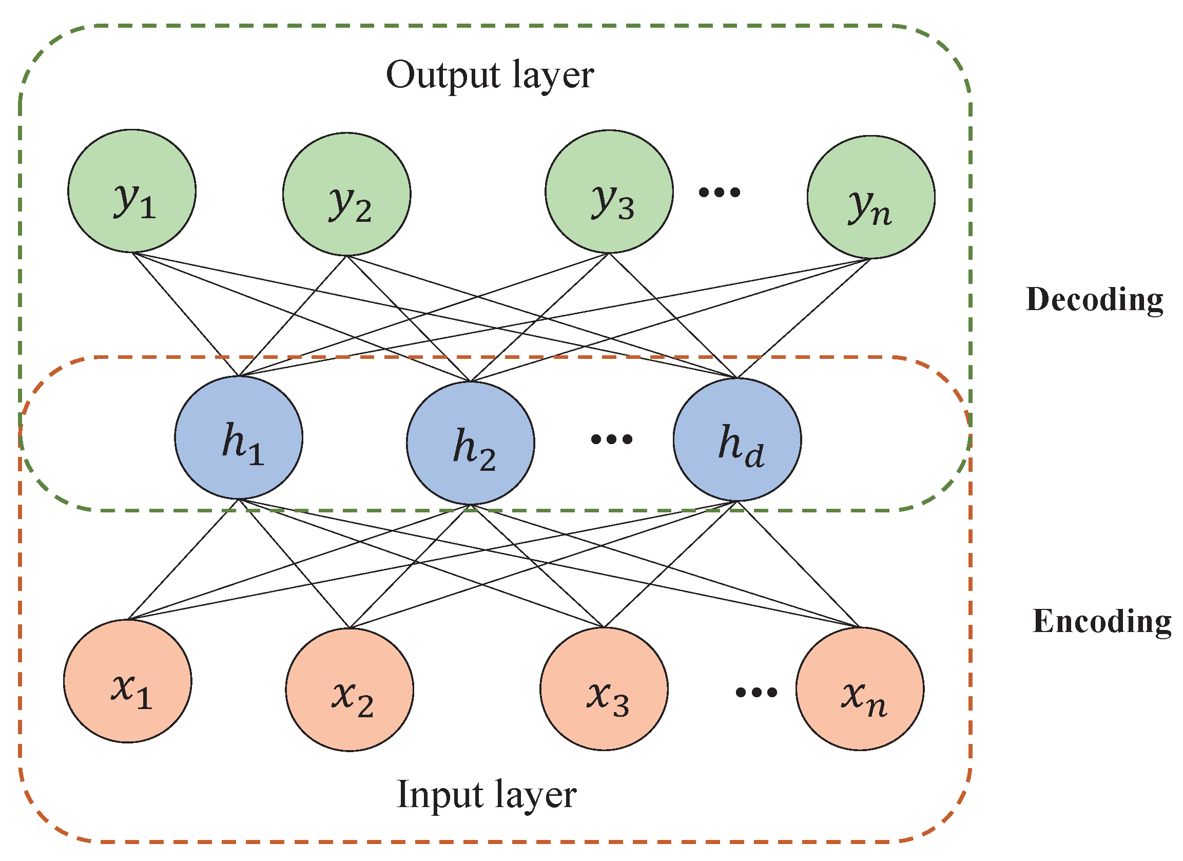
(2) Extraction of Deep Representation Features by AE: For the original signal $\tilde{\mathrm{S}}$ of length L, we first normalize it to eliminate the influence of different feature dimensions as follows:

$${\tilde{\mathrm{S}}}_{\mathrm{norm}}=\frac{\tilde{\mathrm{S}}-{\tilde{\mathrm{S}}}_{min}}{{\tilde{\mathrm{S}}}_{max}-{\tilde{\mathrm{S}}}_{min}}$$

(13)

After the data are normalized, we slice the signal by the specified sample length to obtain multiple samples. In order to better extract the features in the signal, the signal in the time domain is converted into a one-dimensional spectrum, which can be expressed as:

$${\tilde{\mathrm{S}}}_{\mathrm{norm}}^{FFT}=\mathrm{FFT}\left({\tilde{\mathrm{S}}}_{\mathrm{norm}}\right)$$

(14)

where ${\tilde{\mathrm{S}}}_{\mathrm{norm}}$ is the normalized signal; ${\tilde{\mathrm{S}}}_{\mathrm{norm}}^{FFT}$ is the spectral domain signal obtained after fast Fourier transformation (FFT). Taking the signal obtained by FFT as the input of the AE, the encoding process of AE is given as:

$$\mathrm{X}=\mathrm{f}\left({\tilde{\mathrm{S}}}_{\mathrm{norm}}^{FFT}\right)=\sigma \left(\mathrm{W}{\tilde{\mathrm{S}}}_{\mathrm{norm}}^{FFT}+\mathrm{b}\right)$$

(15)

where $\sigma (·)$ is the activation function, $\mathrm{W}$ is the parameter matrix, and b is the bias value. Analogously, the decoding process can be described as:

$$\mathrm{Y}=\mathrm{f}\left(\mathrm{X}\right)=\sigma (\mathrm{WX}+\mathrm{b})$$

(16)

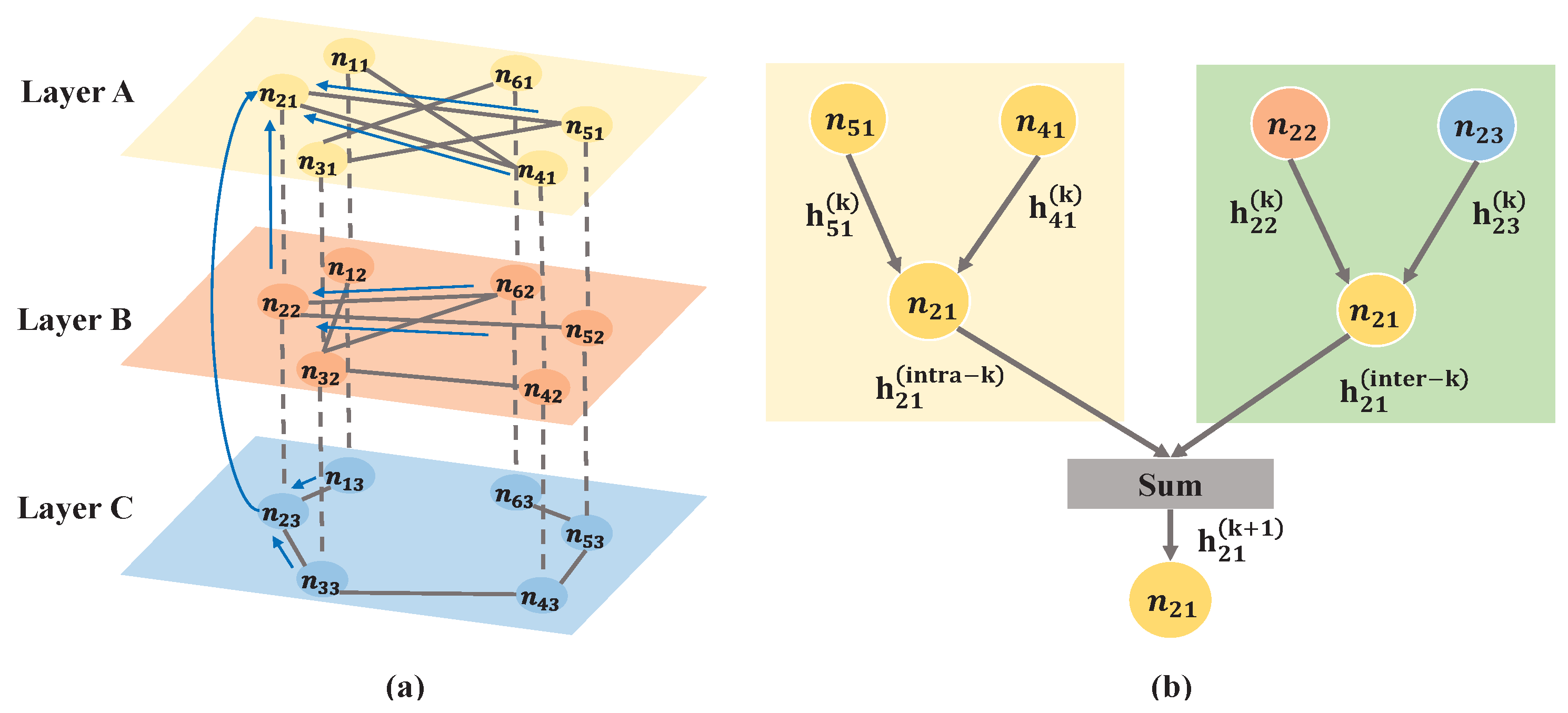
(3) AE-MSGCN-Based Fault Diagnosis: There are multiple potential relationships between the samples in the industrial machine operation process. By using different metrics to calculate the similarity between samples, and then construct the corresponding network structures, the multiple interaction characterization among nodes can be well mined. To achieve this, the feature matrix X obtained through the AE module is input into three different network structures by three different metrics, which are: K-nearest neighbor graph (Layer A), cosine graph (Layer B) and path graph (Layer C). Specifically, in Layer A, the top k nearest neighbors is found for each node by calculating the Euclidean distance between the current node and other nodes as below:

$$S_k=dist(a,b)=\sqrt{\sum _{i=1}^d{\left(a_i-b_i\right)}^2}$$

(17)

Analogously, in Layer B, the k neighbors with the largest similarity are selected to establish edges according to the cosine similarity between the current node and other nodes.

$$S_c=\frac{a·b}{\parallel a\parallel \parallel b\parallel }=\frac{{\displaystyle \sum _{i=1}^d}{a}_i\times b_i}{\sqrt{{\displaystyle \sum _{i=1}^d}{\left(a_i\right)}^2}\times \sqrt{{\displaystyle \sum _{i=1}^d}{\left(b_i\right)}^2}}$$

(18)

where a and b are the feature vectors of any two nodes, and d is the number of nodes. The fault label is also the label of the node.

In Layer C, nodes are connected in chronological order and the nodes at the previous and the next moment of the node are selected as neighbors for the present node. After that, the corresponding adjacency matrixes $A_{\alpha }\in R^{N\times N},\alpha =1,2,3$ can be obtained for different network structures.

The obtained multi-layer networks are taken as the input of the GCN model. Different from the traditional GCN, we replace each GCN layer with multi-convolutional layers, which contain intra-layer convolution and inter-layer convolution, and independently propagate node features within and between layers. The process of intra-layer convolution can be expressed as:

$$\begin{array}{c}{H}_{\mathrm{intra}}^{\alpha }=GCN\left(\mathrm{X},{\mathrm{A}}_{\alpha }\right),\alpha =1,2,3\\ H_{\mathrm{intra}}=CON\left(H_{\mathrm{intra}}^{\alpha }\right)\end{array}$$

(19)

where CON indicates concatenation. By constructing a fully connected graph for the same nodes in each layer, a fully connected graph with N (N is the number of samples) and three vertices can be obtained. Then, the process of inter-layer convolution is given as below:

$$\begin{array}{c}{H}_{\mathrm{inter}}^{\beta }=GCN\left(\mathrm{X},{\mathrm{A}}_{\beta }\right),\beta =1,2,\dots ,\mathrm{N}\\ H_{\mathrm{inter}}=CON\left(H_{\mathrm{inter}}^{\beta }\right)\end{array}$$

(20)

The features within and between layers are aggregated to obtain the multi-layer node embeddings. The process can be expressed as follows.

$$H=Sum\left(H_{\mathrm{intra}},H_{\mathrm{inter}}\right)$$

(21)

The dimension $H\in 3N\times d$; that is, H is composed of the eigenmatrix of the three-layer network.

Then, by summing the eigenmatrices of the multi-layer networks, the aggregated node features are obtained [39].

$${\mathrm{H}}_{\mathrm{Agg}}=Sum\left(H_{\alpha }\right)$$

(22)

where $H_{\alpha }\in N\times d$ is the eigenmatrix corresponding to different layers. The advantage of this model is to decouple intra-layer and inter-layer propagation by learning two sets of GCN parameters, enabling the model to learn about the different importance of the two propagation directions. Finally, the fully connected (FC) network with minimum cross entropy loss (CE) and $softmax$ function are used for model iterative training and fault diagnosis.

To better understand the above procedures, Figure 3 gives the schematic diagram of a multi-layer network and the computation of multi-layer node embeddings (take node $n_{21}$ as an example). Specifically, $i\alpha$ represents the ith node of the $\alpha$ layer. $(\mathrm{intra}-\mathrm{k})$ and $(\mathrm{inter}-\mathrm{k})$ are the kth intra-layer and inter-layer convolutional of GCN, respectively. $h_{i\alpha }^{(k+1)}$ represents the feature of node i in layer $\alpha$ after $k+1$ convolutional aggregations.

(4) Rationality of Multi-layer Network Structure: 

Table 1. The statistical indicators of multi-layer network structure.

	Layer A	Layer B	Layer C
Average degree	8.18550	8.29010	0.99995
Average clustering coefficient	0.30425	0.28521	0
Average shortest path length	18.13	10.79	6667

gives the comparison of the main statistical indicators regarding the multi-layer network structures used in this paper, which is conducted on the Southeast University dataset (SEU). The rationality of the constructed multi-layered networks can be explained in two items:

First, it can be seen from the table that the difference in values of three commonly used evaluation indexes [40] (average degree, average clustering coefficient, average shortest path length) with respect to the multi-layer networks is obvious, especially regarding average shortest path length. That means the multi-layer network structure in this work can depict the complex correlations of process data from different perspectives, which is beneficial to data feature mining and diagnostic performance enhancement. Second, the quantitative effects of multi-layer networks on model performance are shown in detail in Section 4.2, which further proves the availability of the proposed network structure in improving the performance of the diagnostic model.

4. Experimental Results and Analysis

4.1. Dataset Introduction and Experiment Description

(1) Simulated Southeast University Data: The SEU contains two main parts, a gearbox and a bearing, and the experimental setup for the gearbox dataset is shown in Figure 4. The process data of SEU were obtained from the drivetrain dynamic simulator (DDS). In this platform, the fault data includes two working conditions, which correspond to the cases where the speed load is either 20 HZ-0V or 30 HZ-2V, respectively. It is worth noting that there are eight different types of faults for bearings and gearboxes, which are listed in

Table 2. The specific channels and corresponding sensor signals of SEU.

Location	Type	Description
	Chipped	Crack occurs in gear feet
Gearbox	Miss	Missing one of feet in gear
	Root	Crack occurs in root of gear feet
	Surface	Wear occurs in surface of gear
	Ball	Crack occurs in the ball
Bearing	Inner	Crack occurs in inner
	Outer	Crack occurs in outer
	Combination	Crack occurs in both inner and outer

. A detailed description and introduction of the SEU dataset can be found in [41].

(2) Real-World Coal Mill Operation (CMO) Data: The coal mill operation (CMO) data come from the real running process of the coal mill group of a power company in central China. The boiler adopts a medium speed milling system. In addition, each furnace is equipped with 6 $MP265G$ medium speed coal mills. When burning the designed coal type, there are five sets of operation and one set of standby, and the designed coal fineness is $R_{90}=20\%$. The main burners are arranged on the front and back walls of the water-cooled wall, and eight burners on each layer correspond to a coal grinder. The separated over fire air (SOFA) burners are arranged on the front and rear walls of the water wall above the main burner zone to achieve staged combustion to reduce $N{O}_x$ emissions. A recirculating flue gas nozzle is arranged on the front and back walls of the water cooling wall below the burner.

The time span of data collection for the coal mill group is 15 months (from 1 September 2019 to 25 March 2021), with normal data collected every 5 min and fault data collected every 1 s. A total of 32 kinds of faults (given in

Table 3. The main performance parameters of the coal mill.

No.	Description	No.	Description
F1	High pressure of filter screen	F17	Motor abnormalities
F2	The burner burns through	F18	Bearing offset
F3	Abnormal vibration of oil pump	F19	Bearing temperature rise
F4	Hydraulic oil leakage	F20	Vibration is large
F5	The furnace breathed fire	F21	The vibration is noisy
F6	Wind anomalies	F22	Bearing vibration
F7	Powder tube leakage	F23	Powder tube leakage
F8	Loading force becomes smaller	F24	A coal mill vibration
F9	Sudden increase in fan vibration	F25	Electrical short circuit
F10	Hydraulic pressure large	F26	Coal mill current sloshing
F11	Low loading force	F27	Coal mill C vibration
F12	Abnormal loading force	F28	Low inlet wind speed
F13	Low oil pressure	F29	High vibration of fan B
F14	Internal oil leakage	F30	Air preheater current sloshing
F15	Fan surge	F31	Elbow leakage powder
F16	Current is big	F32	Mill C vibration

) were collected in the operating process. Figure 5 gives the physical photo of the $MP265G$ coal mill, which mainly includes primary fan, induced draft fan, air blower, air preheater, and so on. Then the main system parameters of the coal mill are demonstrated in

Table 4. The main performance parameters of CMO dataset with different types of coal.

No.	Description	Unite	Coal Type 1	Coal Type 2 (and 3)
1	Pulverized coal moisture	%	7	3 (6.5)
2	Base point output	t/h	116.1	116.1 (116.1)
3	Maximum ventilation	t/h	154.0	145.0 (176.15)
4	Load ratio	%	63.9	57.7 (67.3)
5	Inlet temperature	°C	292	256 (301)
6	Rotating speed	r/min	27.4	27.4 (27.4)
7	Ventilation resistance	Pa	7100	7000 (7320)
8	Sealed air volume	t/h	8.61	8.61 (8.61)
9	Power consumption	kWh/t	8.82	9.38 (8.43)
10	Wear rate	g/t	4∼6	4∼6 (4∼6)
11	Roller life	h	≥18,000	≥18,000 (≥18,000)
12	Pebble coal amount	kg/h	59	59 (60)
13	Separator diameter	mm	≥4700	≥4700 (≥4700)

.

(3) Experiment Description: The signal data are first subjected to max–min normalization before being input into the model. For the SEU dataset, 128 sampling points are used as a sample; that is, the feature dimension of each sample is 1024, and the initial feature extraction is performed with FFT. For the CMO dataset, each sampling point is taken as a sample, and its feature dimension is 172. The experimental task of the SEU dataset is a 20-class fault classification problem with 1000 samples for each class. The experimental task of the CMO dataset is a 32-class fault classification problem with 800 samples per class. The ratio of training, validation, and testing data sets is 60%:20%:20%, which is divided randomly. For more robust results, each training is performed 10 times on average. The framework is implemented using the Pytorch Geometric (PyG) library [42] and iteratively trained for 300 epochs. The attenuation learning rate is selected here with an initial value of 0.015, and the Adam optimizer is used for optimization in the experiments.

4.2. Visualization Results of AE-MSGCN

In order to display the differences and complementarities among multi-layer networks, Figure 6 demonstrates an example of network topology by different types of metrics for fault Miss${}_{-}{20}_{-}0$ (one kind of Miss fault) in the SEU dataset and F5 in the CMO dataset. In particular, 100 nodes are randomly selected (denoted by solid circles) and the lines with arrows represent learned edges among nodes in the current network. As one can see from the figure, the topology structures of the three-layer networks are quite different from each other, which implies that each metric can learn a specific network structure. Furthermore, the learned network structures also show the differences among different faults. The above results indicate that the AE-MSGCN model with three different metrics can generate expressive fault representations and provide comprehensive fault features, which are naturally helpful in terms of improving fault diagnosis performance.

In order to obtain the best diagnostic performance, comparative experiments are conducted on the two datasets for different hidden layer structures of AE-MSGCN (the size of hidden layer 1 is H and the size of hidden layer 2 is I), which are shown in

Table 5. AE-MSGCN performance with respect to different hidden layer sizes.

SEU			CMO
$H\times I$	Accuracy	Iteration Times	$H\times I$	Accuracy	Iteration Times
$1024\times 128$	96.53%	160	$256\times 128$	98.12%	271
$256\times 128$	95.15%	181	$512\times 256$	99.84%	142
$1024\times 512$	99.75%	177	$128\times 64$	90.76%	288

.

From Table 5, it can be seen that when H = 1024, I = 512, the AE-MSGCN achieved the best diagnostic performance on the SEU dataset (99.75%). When H = 512, I = 256, the GCN obtained the highest fault diagnosis accuracy regarding the CMO dataset (99.84%). Thus, the subsequent results are based on such a hidden layer structure.

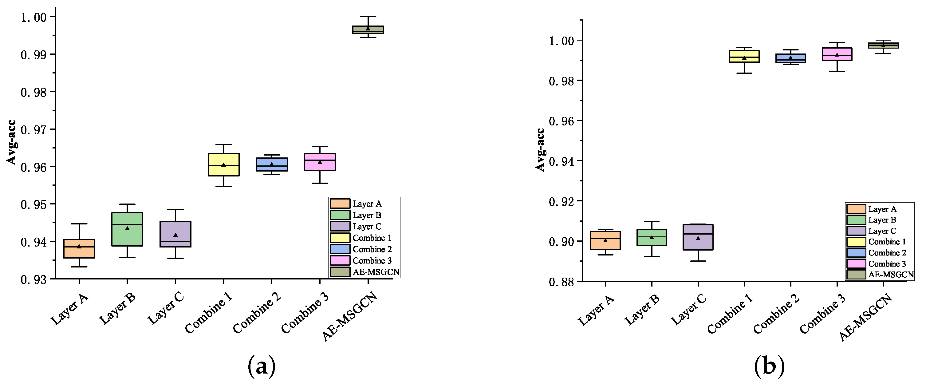
To further quantitatively demonstrate the effects of the multi-layer network structure on the diagnostic performance, comparative experiments are carried out on the two datasets, separately. Each experiment runs 300 epochs and performs 10 times on average. The average diagnosis accuracies (Avg-acc) are shown in Figure 7; it can be seen that the diagnosis accuracy of the combination of multi-layer networks (Layer A + Layer B, Layer A + Layer C, or Layer B + Layer C) is always superior to that of any single layer networks (Layer A, Layer B, or Layer C) in both the SEU dataset and the CMO dataset, which shows that multi-layer networks are helpful for diagnosing performance enhancement. In particular, the proposed AE-MSGCN model utilized three-layer networks to characterize both the intra-and inter-layer relations; thus, the highest diagnosis accuracies are obtained with smaller model variance.

To visualize the training convergence process of the AE-MSGCN model, Figure 8 shows the training loss and testing accuracy curves of AE-MSGCN regarding both SEU and CMO datasets. We can infer from Figure 8 that the loss of AE-MSGCN converged to a stable value after 177 epochs of training, with an accuracy of 99.75% on the testing dataset of SEU. In contrast, after 142 epochs of training on the CMO dataset, the convergence occurred with a diagnosis accuracy of 99.84% without overfitting. In general, the training process of the proposed method is relatively smooth, and the best fault diagnosis accuracy can be achieved with not too many epochs. Thus, it is proved that the proposed method has fast convergence speed and good fault diagnosis performance.

To show the feature visualization results achieved by the proposed AE-MSGCN model, the reduced 2D feature map of raw data and learned fault features in the last layer is visualized in Figure 9 through the t-distributed stochastic neighbor embedding (t-SNE) scheme. From the figure, we know that the sample features of the different faults are crossed and overlapped together in both original SEU/CMO data spaces, which means the faulty pattern is multiple in raw datasets and the interactions between them are complex, especially the SEU dataset. By contrast, the different fault features are well separated with very little overlap after t-SNE mapping, which means the proposed AE-MSGCN model obtains better fault diagnosis performance.

4.3. Comparison and Analysis of Experimental Results

To show the superiority of the proposed AE-MSGCN method, some well-known methods (MLP, GCN, WGCN, MRFGCN) are selected for comparison. The learning rate of these comparison algorithms is 0.015, the Adam operator is used for parameter optimization, and CE is used for iterative training. For fair comparison, all methods are tested under the same conditions. In addition, all methods are trained 10 times to ease the randomness. The best model in the training stage is selected for testing, and the test accuracy is considered as the quantitative evaluation index.

(1) MLP: This is a classical neural network model and it has been verified that MLP has a good performance in fault classification. Thus, it is employed as a baseline to evaluate the effectiveness of AE-MSGCN.

(2) GCN: Differing from MPL, GCN is a DL-based method and the results of the GCN model in this paper are obtained by averaging the diagnosis results obtained by the three single-layer networks constructed by different metrics.

(3) WGCN: This weights the edges by summing the adjacency matrix of multi-layer networks, and then carries out fault diagnosis through GCN. However, it does not consider the aggregation of the features from different neighbors.

(4) MRFGCN: MRFGCN not only extracts the features from different receptive fields, but also fuses them as the enhanced feature representation; thus, it is also an advanced feature mining model. The details can be found in [43].

(5) MSGCN: Compared with the proposed AE-MSGCN, this only lacks the deep feature extraction based on AE. Thus, the validity of AE models can be highlighted.

Subsequently, as for the separability of the AE-MSGCN model concerning the faulty data, the detailed diagnosis results of the two experimental datasets are displayed by using the confusion matrix, which is given in Figure 10. As can be seen from the figure, AE-MSGCN has only a few samples misclassified in both datasets, which can achieve the expected classification effect. After classification, each category has a high degree of discrimination, indicating that AE-MSGCN can correctly identify most of the faults in both of the datasets. Comparing the GCN, MRFGCN, and the AE-MSGCN model, since the GCN model is relatively simple, it only uses single-layer convolution to extract graph features without mining multiple interactions and relations in sensor data, so the fault classification accuracy is not high. In contrast, the AE-MSGCN model carries out the intra-layer and inter-layer convolution to characterize the complex interactions among nodes; thus, the fault classification performance has been further improved.

In order to verify that the proposed method is helpful for fault diagnosis, AE-MSGCN is compared with MLP, GCN, WGCN, MRFGCN [43], and MSGCN; the overall classification results are given in

Table 6. Fault diagnosis accuracy (%) of different methods for the two datasets.

	AE-MSGCN	MSGCN	MRFGCN	WGCN	GCN	MLP
SEU	99.75	98.32	97.25	94.35	94.27	91.32
CMO	99.84	97.33	94.26	91.62	90.05	59.46

. It can be seen from Table 6 that MLP has the worst diagnosis performance. The main reason is that MLP has only two hidden layers, so it cannot effectively extract features. GCN and WGCN only contain intra-layer convolution and ignore inter-layer information among the sensor signals. Although the fault diagnosis accuracy of GCN and WGCN is better than that of MLP, there is still room for improvement. MRFGCN fuses the features from multiple receptive fields to form an enhanced feature representation, and reaches classification accuracies of 97.25% and 94.26% on the two datasets, respectively. In contrast, the proposed AE-MSGCN uses different metrics to form the multi-layer networks and takes into account the feature information among intra-layer and inter-layer sorts; thus, it achieves the excellent diagnosis performance. In addition, the AE model is conducive to the feature extraction of process measurements, which also improves diagnosis accuracy slightly.

Similarly, the standard deviations (SDs) of different methods for the two datasets are shown in

Table 7. The SD (%) of different methods for the two datasets.

	AE-MSGCN	MSGCN	MRFGCN	WGCN	GCN	MLP
SEU	0.14	0.43	0.52	1.25	1.43	2.71
CMO	0.09	0.34	0.6	0.89	1.07	4.93

. From the table, we know that the proposed AE-MSGCN achieves the lowest SD values (i.e., 0.14% for SEU and 0.09% for CMO), which validates the robustness and stability of the proposed method.

Further, we select five categories of faults (Health${}_{-}{20}_{-}0$, Miss${}_{-}{20}_{-}0$, Miss${}_{-}{30}_{-}0$, Root${}_{-}{30}_{-}2$, Outer${}_{-}{20}_{-}0$) in the SEU dataset and the first five faults (F1-F5) as two concrete cases for method validation. It is worth noting that the proposed method achieves 100% fault diagnosis accuracy in all five faults of the SEU dataset, which is superior to any comparison algorithm. A similar situation occurs concerning the CMO dataset. The above comprehensive results demonstrate that the baseline methods cannot completely meet the intelligent diagnosis requirements. A detailed diagnosis and statistical analysis results of the proposed AE-MSGCN approach in different experimental scenarios are clearly shown in Figure 11.

5. Conclusions

Aiming at the problem of ignoring the complex relationships among the industrial machine operation data, this paper designs an innovative way to consider both the inter- and intra-layer influences on fault diagnosis. In the proposed AE-MSGCN, different indicators are used to construct the multi-layer networks. After that, node feature propagation happens in both the intra- and inter- layer independently, then information from the topology and the features farther in the networks are captured by multiple layers; thus, it is beneficial to fault diagnosis performance promotion. The experiments on the simulated SEU dataset and real-world CMO dataset demonstrate that our proposal achieves superior outcomes with regard to fault diagnosis results and model practicability.

Although the proposed method acquires the desired results, the edges of the graph learned by AE-MSGCN are only described by statistical correlations. Further efforts could be focused on the design of multi-layer networks with interpretability and nodes with physical significance. In addition, the potential integration of the diagnosis framework into software systems is also worth addressing in future works.