
An Improved Sparrow Search Algorithm for Solving the Energy-Saving Flexible Job Shop Scheduling Problem


Abstract
:1. Introduction
- It is rare to find relevant papers on the FJSP with the consideration of energy-saving constraints and the optimization criterion of minimizing the total power consumption cost. With energy-saving concerns, this study aims to fill in this research gap by defining, modelling, and solving the EFJSP.
- To efficiently solve the EFJSP, we developed an improved sparrow search algorithm (ISSA) that consists of the hybrid search (HS), quantum rotation gate (QRG), sine–cosine algorithm (SCA), adaptive adjustment strategy (AAS), and variable neighborhood search (VNS) techniques.
- The advantages of the developed ISSA are verified by extensive computational experiments on benchmark and practical instances.
- The purpose of this paper is to increase knowledge reserves in the field of energy-saving scheduling in theory and to help manufacturing enterprises reduce energy consumption and processing costs in practice.
2. EFJSP Description
2.1. Problem Description
- (1)
- One machine can deal with only one operation at a time.
- (2)
- One operation must be machined continuously, as it cannot be interrupted midway.
- (3)
- There are sequential constraints among the operations of the same job, as it can start only after the previous one is completed.
- (4)
- Different operations of all jobs are independent.
- (5)
- There is no interruption when the machine is available.
- (6)
- The preparation of the machine before processing, loading, and unloading of the job is ignored.
- (7)
- Machine failure and other emergencies are not considered.
2.2. Model Illustration
3. Sparrow Search Algorithm (SSA)
4. Our Proposed Improved Sparrow Search Algorithm (ISSA)
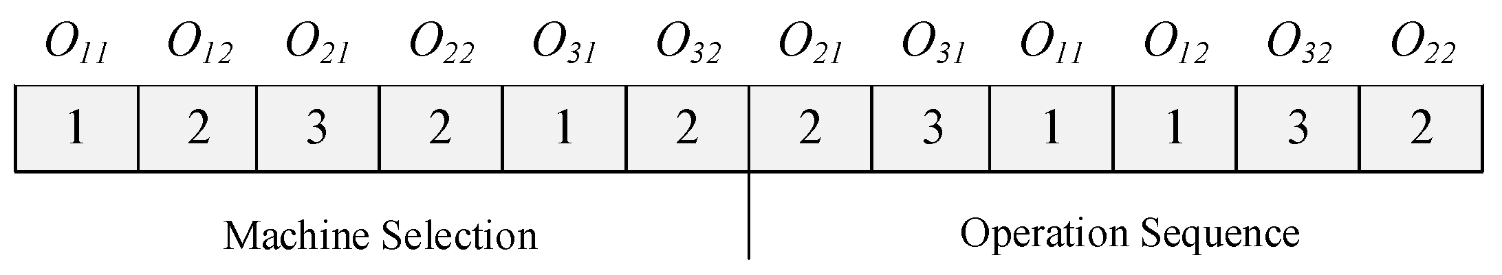
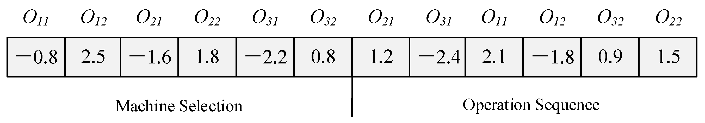
4.1. Scheduling Scheme Denotation
4.2. Individual Position Vector
4.3. Transition Mechanism
4.3.1. Transition from SS to IPV
- (1)
- Machine selection segment: the transition procedure is shown in Equation (5).where represents the ith data of the IPV. defines the number of machines that can be selected for the corresponding operation of the ith element. indicates the selected machine’s serial number; if , then can take any value in the interval .
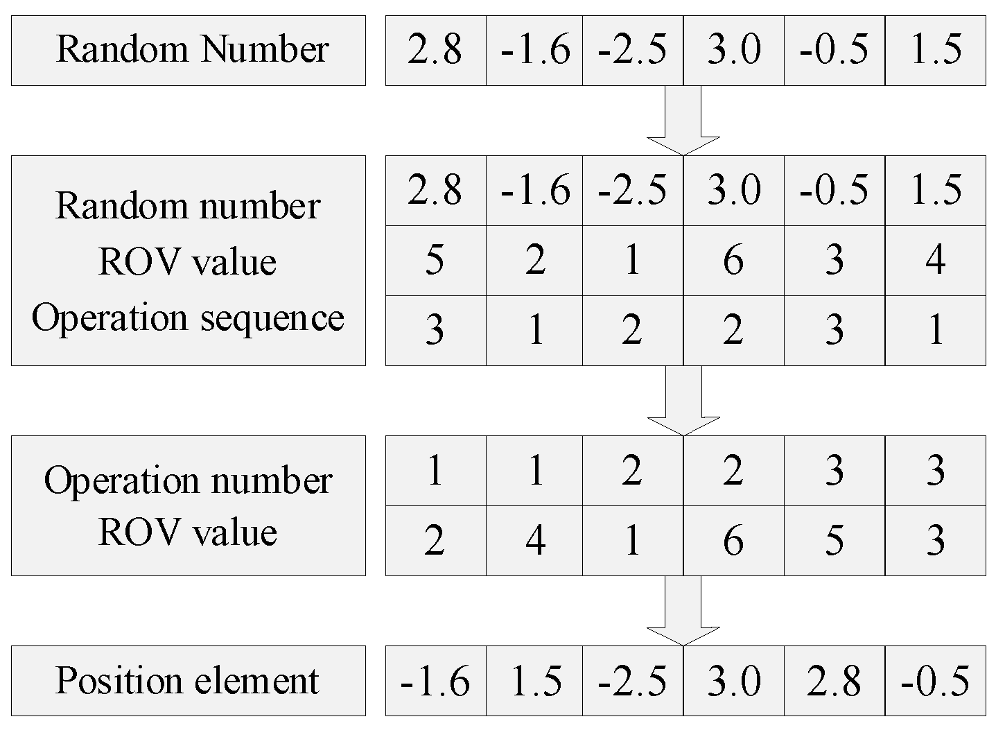
- (2)
- Operation sequence segment: firstly, the real numbers (detonated by ) are randomly produced between for the SS. Based on the ranked-order-value (ROV) rule, we can allocate one unique ROV datapoint for each real number produced before in an ascending sequence; hence, the ROV datapoint can map to one operation. Then, the ROV datapoint is re-ordered on the basis of the sequence of the operations, and the real number is also re-ordered according to the re-ordered ROV datapoint, which is the data value in the IPV. The transition procedure can be described as Figure 4.
4.3.2. Transition from IPV to SS
- (1)
- Machine selection part: based on the reverse derivation of Equation (5), the transformation can be implemented by Equation (6).
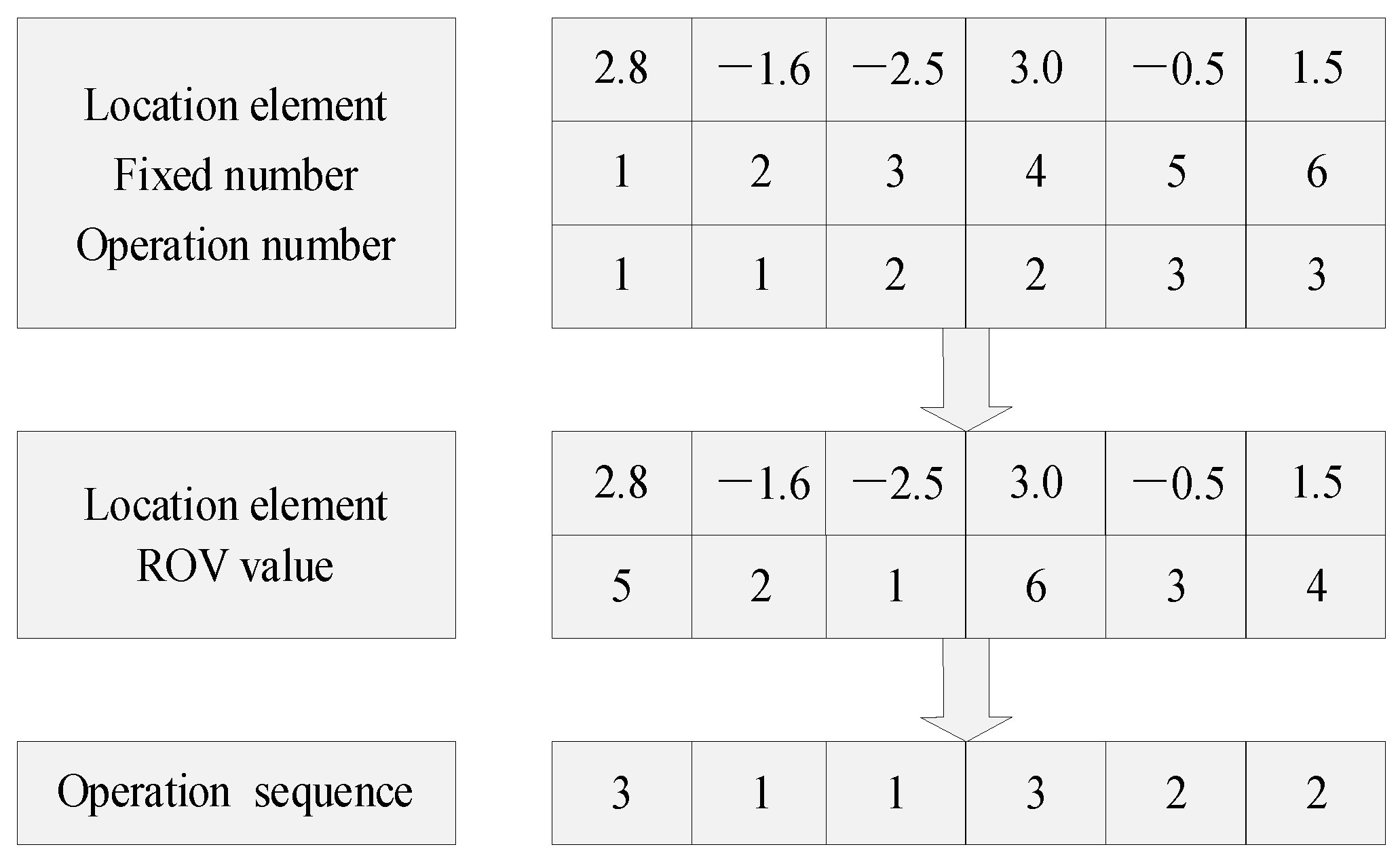
- (2)
- Operation sequence part: We assign an ROV datapoint to each element of the IPV in ascending order. Then, the ROV datapoint is used as the fixed position number. Finally, the operation permutation can be achieved by matching the ROV datapoint to the operations. The conversion process is described in Figure 5 as follows:
4.4. Population Initialization
4.5. Dynamic Weights and Quantum Rotation Gate
4.6. Sine–Cosine Algorithm
4.7. Adaptive Adjustment Strategy
4.8. Variable Neighborhood Search
- Step 1.
- Set the current best scheduling scheme as the original scheme , and set the threshold , , and termination condition .
- Step 2.
- If , set as ; if , set as .
- Step 3.
- If , then set as ; if not, set as .
- Step 4.
- Set as , if , then set as , and go to Step 5; if not, return to Step 2.
- Step 5.
- End.
4.9. Parameters of the ISSA
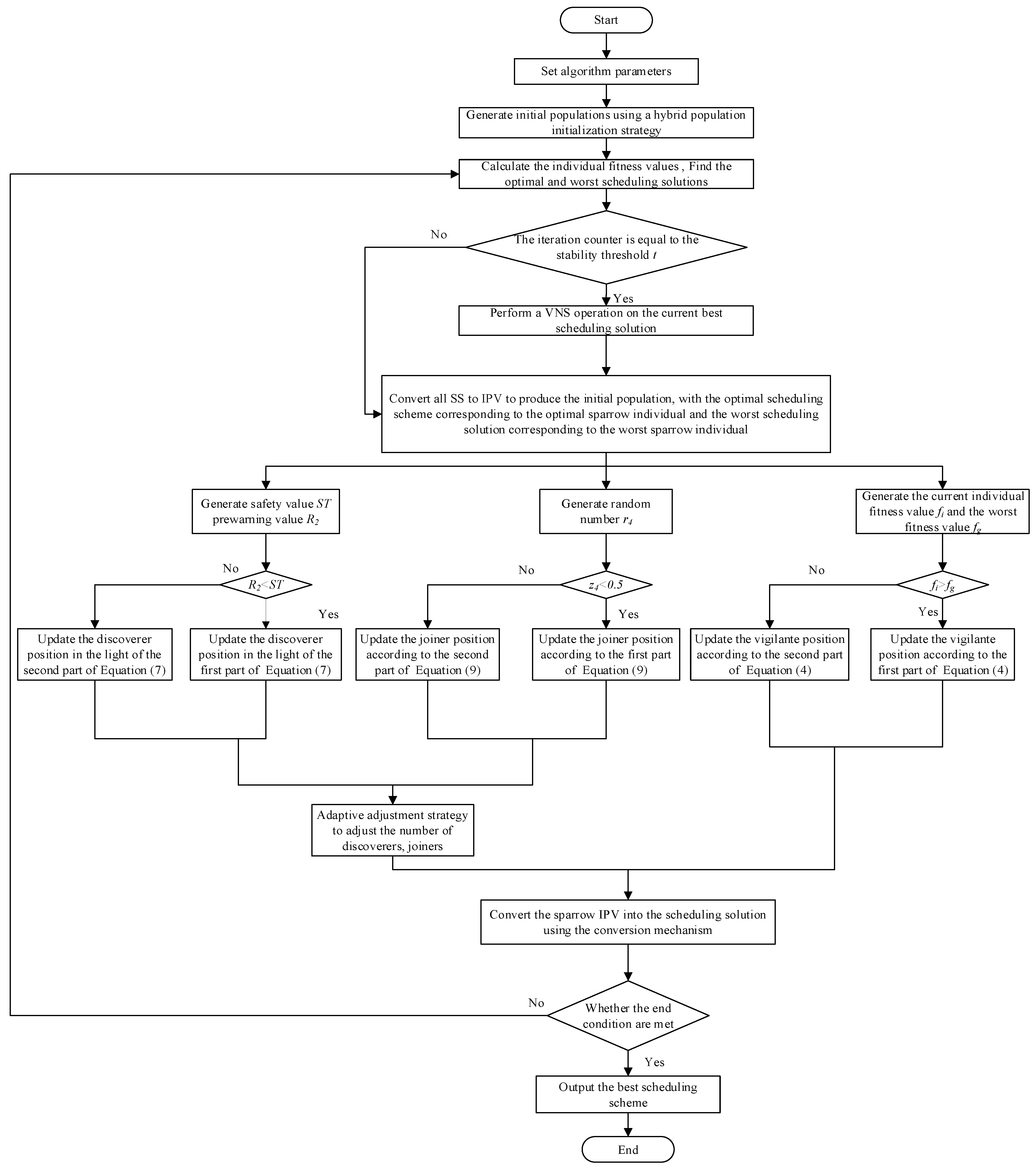
4.10. Procedure of the ISSA
- Step 1.
- Set parameters and produce the original swarm by using the HS.
- Step 2.
- Determine the objective function values of all scheduling schemes, and then search the optimal and worst schemes.
- Step 3.
- Determine whether the optimal scheduling scheme is in a steady state; if so, execute the VSN on it; otherwise, go to Step 5.
- Step 4.
- Perform the conversion from scheduling scheme to IPV, and retain corresponding to and the worst individual position vector corresponding to the worst scheduling scheme .
- Step 5.
- Regenerate the discoverer’s positions based on Equation (7), the joiner’s positions based on Equation (9), and the guarder’s positions based on Equation (4).
- Step 6.
- Adjust the number of discoverers and joiners using the adaptive adjustment strategy.
- Step 7.
- A conversion mechanism is used to convert the updated IPV in the population to the scheduling scheme; then, find the optimal scheduling scheme.
- Step 8.
- Judge whether the stopping condition is met; if so, output ; otherwise, return to Step 2.
5. Computational Experiments
5.1. Experimental Settings
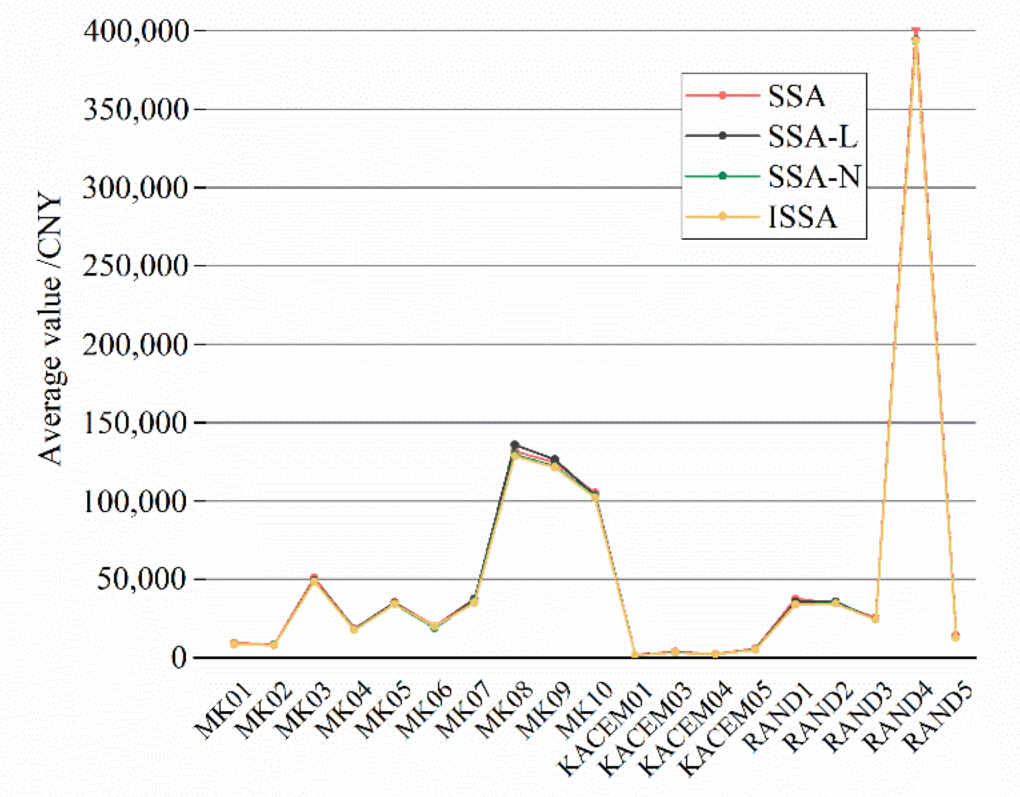
5.2. Effectiveness of Enhancement Strategies
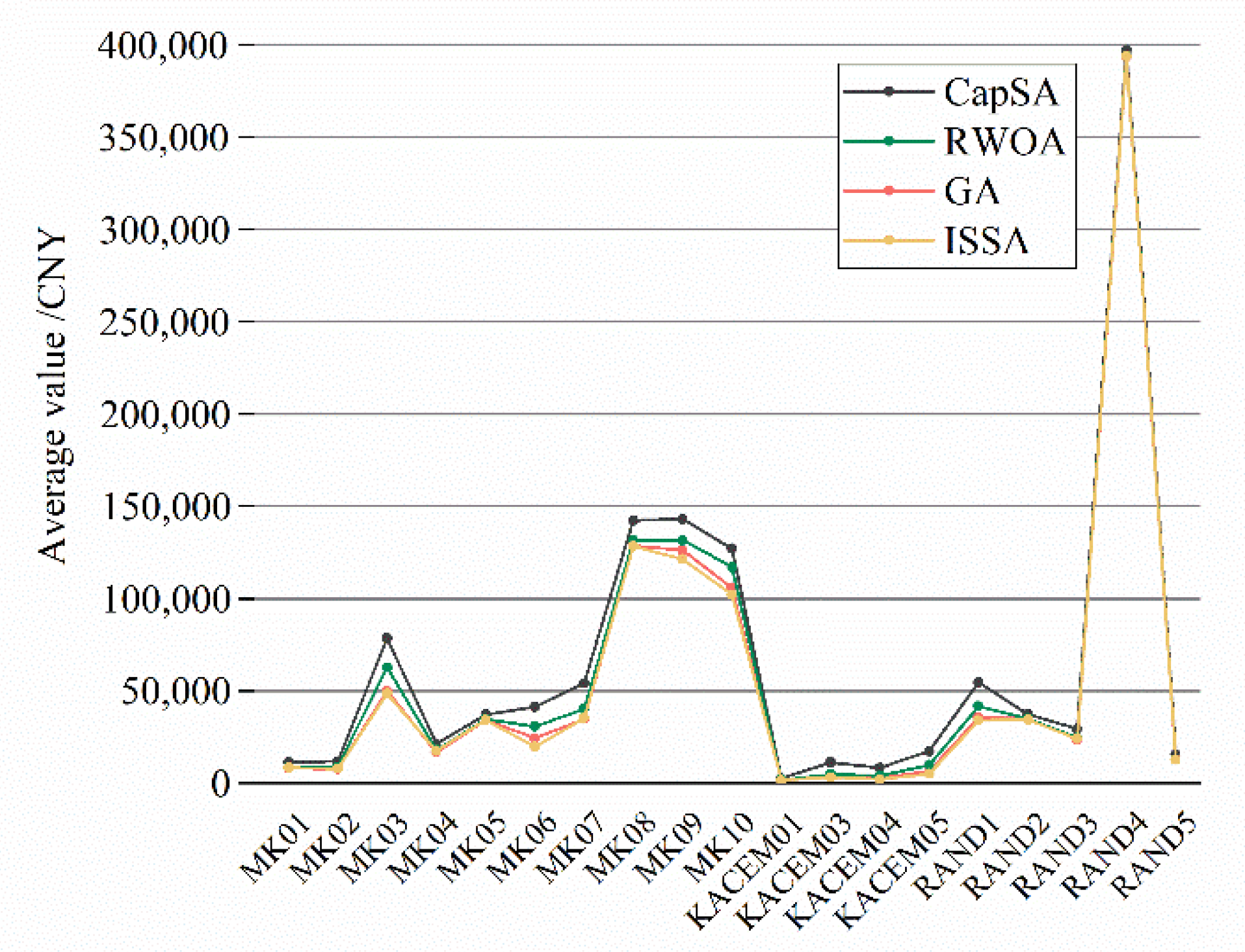
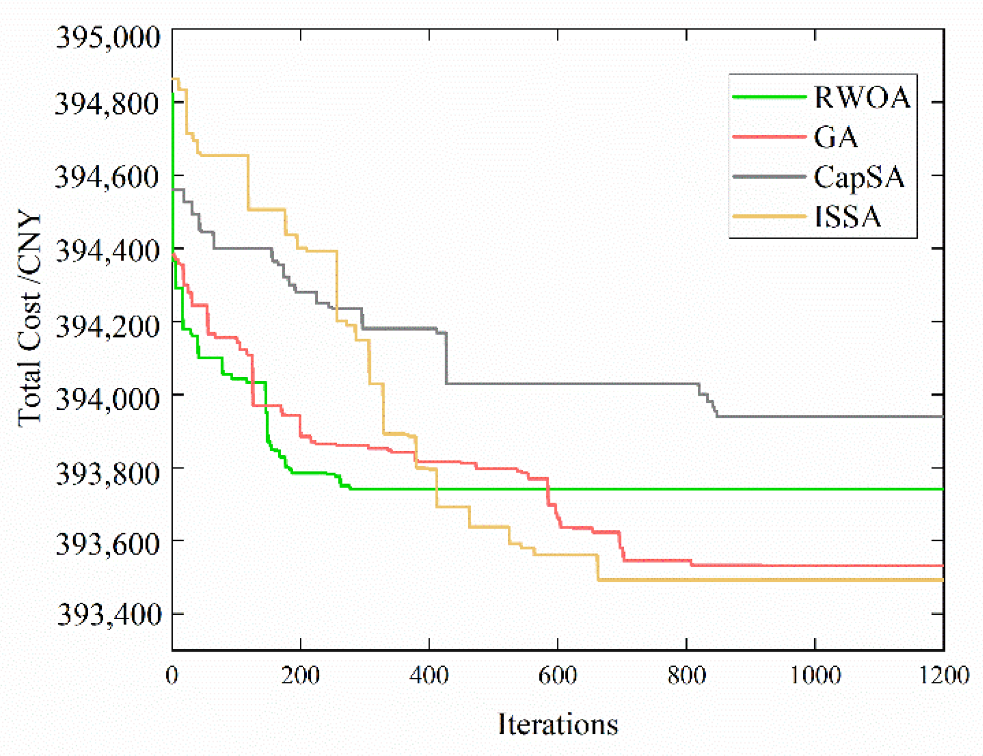
5.3. Comparison with Existing Algorithms
6. Conclusions
Author Contributions
Funding
Data Availability Statement
Conflicts of Interest
References
- Kim, D.H.; Kim, T.J.Y.; Wang, X.; Kim, M.; Quan, Y.J.; Oh, J.W.; Min, S.H.; Kim, H.; Bhandari, B.; Yang, I.; et al. Smart machining process using machine learning: A review and perspective on machining industry. Int. J. Precis. Eng. Manuf.-Green Technol. 2018, 5, 555–568. [Google Scholar] [CrossRef]
- Angelopoulos, A.; Michailidis, E.T.; Nomikos, N.; Trakadas, P.; Hatziefremidis, A.; Voliotis, S.; Zahariadis, T. Tackling faults in the industry 4.0 era—A survey of machine-learning solutions and key aspects. Sensors 2019, 20, 109. [Google Scholar] [CrossRef] [PubMed]
- Fang, K.; Uhan, N.; Zhao, F.; Sutherland, J.W. A new shop scheduling approach in support of sustainable manufacturing. In Glocalized Solutions for Sustainability in Manufacturing; Springer: Berlin/Heidelberg, Germany, 2011; pp. 305–310. [Google Scholar]
- Duflou, J.R.; Sutherland, J.W.; Dornfeld, D.; Herrmann, C.; Jeswiet, J.; Kara, S.; Hauschild, M.; Kellens, K. Towards energy and resource efficient manufacturing: A processes and systems approach. CIRP Ann. Manuf. Technol. 2012, 61, 587–609. [Google Scholar] [CrossRef]
- Carli, R.; Dotoli, M.; Digiesi, S.; Facchini, F.; Mossa, G. Sustainable scheduling of material handling activities in labor-intensive warehouses: A decision and control model. Sustainability 2020, 12, 3111. [Google Scholar] [CrossRef]
- Zhang, L.; Deng, Q.; Gong, G.; Han, W. A new unrelated parallel machine scheduling problem with tool changes to minimise the total energy consumption. Int. J. Prod. Res. 2020, 58, 6826–6845. [Google Scholar] [CrossRef]
- Ahmadi, E.; Zandieh, M.; Farrokh, M.; Emami, S.M. A multi objective optimization approach for flexible job shop scheduling problem under random machine breakdown by evolutionary algorithms. Comput. Oper. Res. 2016, 73, 56–66. [Google Scholar] [CrossRef]
- Salido, M.A.; Escamilla, J.; Giret, A.; Barber, F. A genetic algorithm for energy-efficiency in job-shop scheduling. Int. J. Adv. Manuf. Technol. 2016, 85, 1303–1314. [Google Scholar] [CrossRef]
- Li, Y.; Huang, W.; Wu, R.; Guo, K. An improved artificial bee colony algorithm for solving multi-objective low-carbon flexible job shop scheduling problem. Appl. Soft Comput. 2020, 95, 106544. [Google Scholar] [CrossRef]
- Zhang, X.; Ji, Z.; Wang, Y. An improved SFLA for flexible job shop scheduling problem considering energy consumption. Mod. Phys. Lett. B 2018, 32, 1840112. [Google Scholar] [CrossRef]
- Shahrabi, J.; Adibi, M.A.; Mahootchi, M. A reinforcement learning approach to parameter estimation in dynamic job shop scheduling. Comput. Ind. Eng. 2017, 110, 75–82. [Google Scholar] [CrossRef]
- Yang, W.; Su, J.; Yao, Y.; Yang, Z.; Yuan, Y. A novel hybrid whale optimization algorithm for flexible job-shop scheduling problem. Machines 2022, 10, 618. [Google Scholar] [CrossRef]
- Wu, X.; Sun, Y. A green scheduling algorithm for flexible job shop with energy-saving measures. J. Clean. Prod. 2018, 172, 3249–3264. [Google Scholar] [CrossRef]
- Zhu, J.; Shao, Z.H.; Chen, C. An improved whale optimization algorithm for job-shop scheduling based on quantum computing. Int. J. Simul. Model. 2019, 18, 521–530. [Google Scholar] [CrossRef]
- Anuar, N.I.; Fauadi, M.; Saptari, A. Performance evaluation of continuous and discrete particle swarm optimization in job-shop scheduling problems. IOP Conf. Ser. Mater. Sci. Eng. 2019, 530, 012044. [Google Scholar] [CrossRef]
- Ding, J.Y.; Song, S.; Wu, C. Carbon-efficient scheduling of flow shops by multi-objective optimization. Eur. J. Oper. Res. 2016, 248, 758–771. [Google Scholar] [CrossRef]
- Yang, J.; Xu, H. Hybrid memetic algorithm to solve multiobjective distributed fuzzy flexible job shop scheduling problem with transfer. Processes 2022, 10, 1517. [Google Scholar] [CrossRef]
- Dai, M.; Tang, D.; Giret, A.; Salido, M.A. Multi-objective optimization for energy-efficient flexible job shop scheduling problem with transportation constraints. Robot. Comput.-Integr. Manuf. 2019, 59, 143–157. [Google Scholar] [CrossRef]
- Tan, W.; Yuan, X.; Wang, J.; Zhang, X. A fatigue-conscious dual resource constrained flexible job shop scheduling problem by enhanced NSGA-II: An application from casting workshop. Comput. Ind. Eng. 2021, 160, 107557. [Google Scholar] [CrossRef]
- Lu, C.; Li, X.; Gao, L.; Liao, W.; Yi, J. An effective multi-objective discrete virus optimization algorithm for flexible job-shop scheduling problem with controllable processing times. Comput. Ind. Eng. 2017, 104, 156–174. [Google Scholar] [CrossRef]
- Carli, R.; Digiesi, S.; Dotoli, M.; Facchini, F. A control strategy for smart energy charging of warehouse material handling equipment. Procedia Manuf. 2020, 42, 503–510. [Google Scholar] [CrossRef]
- Yin, L.; Li, X.; Gao, L.; Lu, C.; Zhang, Z. A novel mathematical model and multi-objective method for the low-carbon flexible job shop scheduling problem. Sustain. Comput. Inform. Syst. 2017, 13, 15–30. [Google Scholar] [CrossRef]
- Choudhury, A. The role of machine learning algorithms in materials science: A state of art review on industry 4.0. Arch. Comput. Method E 2021, 28, 3361–3381. [Google Scholar] [CrossRef]
- Angelopoulos, A.; Giannopoulos, A.; Spantideas, S.; Kapsalis, N.; Trochoutsos, C.; Voliotis, S.; Trakadas, P. Allocating orders to printing machines for defect minimization: A comparative machine learning approach. In Proceedings of the International Conference on Artificial Intelligence Applications and Innovations, Crete, Greece, 17–20 June 2022; Springer: Cham, Switzerland, 2022; pp. 79–88. [Google Scholar]
- Wang, G.G.; Gandomi, A.H.; Alavi, A.H. An effective krill herd algorithm with migration operator in biogeography-based optimization. Appl. Math. Model. 2014, 38, 2454–2462. [Google Scholar] [CrossRef]
- Jiang, T.; Zhang, C. Application of grey wolf optimization for solving combinatorial problems: Job shop and flexible job shop scheduling cases. IEEE Access 2018, 6, 26231–26240. [Google Scholar] [CrossRef]
- Han, Y.; Gong, D.; Jin, Y.; Pan, Q. Evolutionary multi-objective blocking lot-streaming flow shop scheduling with machine breakdowns. IEEE Trans. Cybern. 2017, 49, 184–197. [Google Scholar] [CrossRef]
- Li, J.; Duan, P.; Sang, H.; Wang, S.; Liu, Z.; Duan, P. An efficient optimization algorithm for resource-constrained steel-making scheduling problems. IEEE Access 2018, 6, 33883–33894. [Google Scholar] [CrossRef]
- Braik, M.; Sheta, A.; Al-Hiary, H. A novel meta-heuristic search algorithm for solving optimization problems: Capuchin search algorithm. Neural Comput. Appl. 2021, 33, 2515–2547. [Google Scholar] [CrossRef]
- Fan, J.; Li, Y.; Wang, T. An improved African vultures optimization algorithm based on tent chaotic mapping and time-varying mechanism. PLoS ONE 2021, 16, e0260725. [Google Scholar] [CrossRef]
- Odili, J.B.; Mohmad Kahar, M.N.; Noraziah, A. Parameters-tuning of PID controller for automatic voltage regulators using the African buffalo optimization. PLoS ONE 2017, 12, e0175901. [Google Scholar] [CrossRef]
- Ling, Y.; Zhou, Y.; Luo, Q. Lévy flight trajectory-based whale optimization algorithm for global optimization. IEEE Access 2017, 5, 6168–6186. [Google Scholar] [CrossRef]
- Lyu, S.; Li, Z.; Huang, Y.; Wang, J.; Hu, J. Improved self-adaptive bat algorithm with step-control and mutation mechanisms. J. Comput. Sci. 2019, 30, 65–78. [Google Scholar] [CrossRef]
- Verma, O.P.; Aggarwal, D.; Patodi, T. Opposition and dimensional based modified firefly algorithm. Expert Syst. Appl. 2016, 44, 168–176. [Google Scholar] [CrossRef]
- Goings, J.J.; Li, X. An atomic orbital based real-time time-dependent density functional theory for computing electronic circular dichroism band spectra. J. Phys. Chem. C 2016, 144, 234102. [Google Scholar] [CrossRef]
- Xue, J.; Shen, B. A novel swarm intelligence optimization approach: Sparrow search algorithm. Syst. Sci. Control Eng. 2020, 8, 22–34. [Google Scholar] [CrossRef]
- Zhang, C.; Ding, S. A stochastic configuration network based on chaotic sparrow search algorithm. Knowl.-Based Syst. 2021, 220, 106924. [Google Scholar] [CrossRef]
- Ouyang, C.; Qiu, Y.; Zhu, D. A multi-strategy improved sparrow search algorithm. J. Phys. Conf. Ser. 2021, 1848, 012042. [Google Scholar] [CrossRef]
- Zhang, J.; Xia, K.; He, Z.; Yin, Z.; Wang, S. Semi-supervised ensemble classifier with improved sparrow search algorithm and its application in pulmonary nodule detection. Math. Probl. Eng. 2021, 2021, 6622935. [Google Scholar] [CrossRef]
- Liu, G.; Shu, C.; Liang, Z.; Peng, B.; Cheng, L. A modified sparrow search algorithm with application in 3d route planning for UAV. Sensors 2021, 21, 1224. [Google Scholar] [CrossRef]
- Yuan, J.; Zhao, Z.; Liu, Y.; He, B.; Wang, L.; Xie, B.; Gao, Y. DMPPT control of photovoltaic microgrid based on improved sparrow search algorithm. IEEE Access 2021, 9, 16623–16629. [Google Scholar] [CrossRef]
- Zhang, Z.; Han, Y. Discrete sparrow search algorithm for symmetric traveling salesman problem. Appl. Soft Comput. 2022, 118, 108469. [Google Scholar] [CrossRef]
- Yuan, Y.; Xu, H.; Yang, J.D. A hybrid harmony search algorithm for the flexible job shop scheduling problem. Appl. Soft Comput. 2013, 13, 3259–3272. [Google Scholar] [CrossRef]
- Zhang, G.H.; Gao, L.; Li, P.; Zhang, C.Y. Improved genetic algorithm for the flexible job-shop scheduling problem. J. Mech. Eng. 2009, 45, 145–151. [Google Scholar] [CrossRef]
- Wu, H.; Zhang, A.; Han, Y.; Nan, J.; Li, K. Fast stochastic configuration network based on an improved sparrow search algorithm for fire flame recognition. Knowl.-Based Syst. 2022, 245, 108626. [Google Scholar] [CrossRef]
- Liu, S.Q.; Kozan, E.; Corry, P.; Masoud, M.; Luo, K. A real-world mine excavators timetabling methodology in open-pit mining. Opt. Eng. 2022, in press. [CrossRef]
- Luan, F.; Cai, Z.; Wu, S.; Liu, S.Q.; He, Y. Optimizing the low-carbon flexible job shop scheduling problem with discrete whale optimization algorithm. Mathematics 2019, 7, 688. [Google Scholar] [CrossRef]
- Liu, S.Q.; Kozan, E.; Masoud, M.; Zhang, Y.; Chan, F.T. Job shop scheduling with a combination of four buffering constraints. Int. J. Prod. Res. 2018, 56, 3274–3293. [Google Scholar] [CrossRef]
- Liu, S.Q.; Kozan, E. Parallel-identical-machine job-shop scheduling with different stage-dependent buffering requirements. Comput. Oper. Res. 2016, 74, 31–41. [Google Scholar] [CrossRef]
- Liu, S.Q.; Kozan, E. Scheduling trains with priorities: A no-wait blocking parallel-machine job-shop scheduling model. Transp. Sci. 2011, 45, 175–198. [Google Scholar] [CrossRef]
- Liu, S.Q.; Kozan, E. Scheduling trains as a blocking parallel-machine job shop scheduling problem. Comput. Oper. Res. 2009, 36, 2840–2852. [Google Scholar] [CrossRef]
- Liu, S.Q.; Kozan, E. Scheduling a flow shop with combined buffer conditions. Int. J. Prod. Econ. 2009, 117, 371–380. [Google Scholar] [CrossRef]
- Masoud, M.; Kozan, E.; Kent, G.; Liu, S.Q. An integrated approach to optimise sugarcane rail operations. Comput. Ind. Eng. 2016, 98, 211–220. [Google Scholar] [CrossRef]
- Masoud, M.; Kozan, E.; Kent, G.; Liu, S.Q. A new constraint programming approach for optimising a coal rail system. Opt. Lett. 2017, 11, 725–738. [Google Scholar] [CrossRef] [Green Version]


| Job Number | Operations | Machine Candidates | (Processing Time/min, Energy Consumption Cost/CNY) |
|---|---|---|---|
| J1 | O11 | M1, M4 | (7, 12), (8, 18) |
| O12 | M1, M2, M3 | (10, 15), (4, 21), (5, 26) | |
| J2 | O13 | M1, M2, M3, M4 | (5, 14), (3, 16), (4, 17), (6, 18) |
| O21 | M1, M5 | (7, 26), (4, 13) | |
| O22 | M2, M3, M4 | (8, 27), (6, 15), (5, 30) | |
| J3 | O31 | M2 | (6, 17) |
| O32 | M1, M3, M4 | (4, 22), (8, 18), (6, 25) | |
| O33 | M1, M2 | (6, 14), (3, 24), (5, 15) |
| Machine Tool Number | M1 | M2 | M3 | M4 |
|---|---|---|---|---|
| M1 | 0 | 2 | 4 | 3 |
| M2 | 2 | 0 | 5 | 6 |
| M3 | 4 | 5 | 0 | 2 |
| M4 | 3 | 6 | 2 | 0 |
| Instances | SSA | SSA-L | SSA-N | ISSA | ||||
|---|---|---|---|---|---|---|---|---|
| Best | Avg | Best | Avg | Best | Avg | Best | Avg | |
| MK01 | 9306.94 | 9412.82 | 8423.30 | 8447.81 | 8356.37 | 8456.38 | 8446.75 | 8468.81 |
| MK02 | 8347.20 | 8572.23 | 8104.27 | 8130.34 | 8083.54 | 8121.77 | 7985.84 | 8009.98 |
| MK03 | 50,733.22 | 51,119.39 | 48,360.57 | 49,411.72 | 47,461.04 | 48,657.46 | 47,516.67 | 48,661.04 |
| MK04 | 18,298.14 | 18,547.69 | 18,168.26 | 18,226.60 | 17,592.43 | 17,945.63 | 17,045.56 | 17,592.43 |
| MK05 | 35,375.73 | 35,385.59 | 34,864.24 | 35,007.48 | 34,027.61 | 34,270.79 | 34,031.91 | 34,213.75 |
| MK06 | 19,846.10 | 19,968.66 | 19,019.45 | 19,098.94 | 18,963.17 | 19,001.45 | 19,063.16 | 19,859.96 |
| MK07 | 37,695.08 | 37,733.89 | 36,634.76 | 37,397.92 | 35,363.06 | 36,213.89 | 35,254.10 | 35,309.76 |
| MK08 | 131,569.25 | 131,878.23 | 130,738.76 | 135,822.34 | 128,607.15 | 129,560.34 | 127,846.40 | 128,512.99 |
| MK09 | 123,380.55 | 124,448.64 | 123,133.18 | 126,347.35 | 120,314.60 | 122,087.53 | 120,320.29 | 121,351.59 |
| MK10 | 10,4048.53 | 10,5219.69 | 10,3219.69 | 103,533.07 | 102,862.10 | 103,107.89 | 10,0520.95 | 102,149.47 |
| KACEM01 | 1719.85 | 1766.01 | 1711.07 | 1755.18 | 1708.87 | 1758.33 | 1698.76 | 1709.16 |
| KACEM03 | 3344.44 | 3782.32 | 3324.51 | 3381.08 | 3233.20 | 3329.01 | 3245.58 | 3282.17 |
| KACEM04 | 2225.47 | 2336.26 | 2032.63 | 2194.02 | 2137.79 | 2147.11 | 2102.87 | 2129.75 |
| KACEM05 | 5548.58 | 5782.85 | 5140.64 | 5281.19 | 5131.95 | 5206.73 | 5026.08 | 5149.68 |
| RAND1 | 37,144.15 | 37,782.68 | 35,409.28 | 35,849.80 | 33,843.79 | 34,192.36 | 33,224.26 | 34,110.69 |
| RAND2 | 34,004.41 | 34,478.71 | 34,060.55 | 35,808.71 | 34,886.18 | 34,899.45 | 34,118.03 | 34,464.93 |
| RAND3 | 24,803.20 | 25,542.66 | 24,191.84 | 24,265.08 | 24,100.04 | 24,221.53 | 24,102.66 | 24,180.50 |
| RAND4 | 394,304.13 | 401,434.71 | 394,006.28 | 394,110.82 | 393,320.88 | 393,514.54 | 393,409.55 | 393,679.24 |
| RAND5 | 12,980.70 | 14,326.92 | 12,703.42 | 12,863.33 | 12,661.15 | 12,713.42 | 12,640.98 | 12,669.47 |
| Instances | GA | CapSA | ||||||
|---|---|---|---|---|---|---|---|---|
| Best | Avg | SD | ARPD | Best | Avg | SD | ARPD | |
| MK01 | 8123.73 | 8187.99 | 42.41 | 10.12 | 11,289.27 | 11,446.43 | 91.25 | 0.24 |
| MK02 | 7766.51 | 7797.67 | 18.34 | 13.56 | 11,350.54 | 11,907.87 | 331.92 | 0.10 |
| MK03 | 49,827.54 | 49,956.50 | 82.08 | 9.02 | 76,999.30 | 78,509.15 | 881.21 | 0.11 |
| MK04 | 16,788.86 | 16,807.41 | 12.57 | 11.38 | 20,528.32 | 21,372.75 | 573.87 | 0.84 |
| MK05 | 34,174.43 | 34,226.93 | 33.34 | 3.00 | 36725.73 | 37,163.20 | 234.86 | 0.69 |
| MK06 | 23,949.19 | 24,505.27 | 361.59 | 13.54 | 40,674.46 | 41,389.38 | 416.04 | 0.25 |
| MK07 | 34,562.44 | 34,772.24 | 141.56 | 12.90 | 53,566.50 | 54,177.84 | 365.71 | 0.41 |
| MK08 | 127,959.83 | 128,559.31 | 374.17 | 1.20 | 140,882.04 | 142,364.34 | 839.36 | 0.55 |
| MK09 | 125,155.91 | 126,208.61 | 642.92 | 7.30 | 141,528.49 | 143,081.35 | 968.67 | 0.16 |
| MK10 | 104,807.56 | 105,840.88 | 586.53 | 8.60 | 125,612.11 | 127,089.44 | 872.51 | 0.31 |
| KACEM01 | 1739.73 | 1851.74 | 60.05 | 21.20 | 2529.61 | 2598.56 | 40.82 | 0.72 |
| KACEM03 | 3462.67 | 3500.58 | 23.51 | 46.80 | 9972.03 | 11,349.15 | 796.08 | 0.33 |
| KACEM04 | 2734.46 | 2817.20 | 53.17 | 25.67 | 7971.42 | 8362.48 | 258.13 | 0.64 |
| KACEM05 | 6333.49 | 6486.55 | 92.35 | 18.90 | 16,196.32 | 17,292.33 | 657.44 | 0.23 |
| RAND1 | 35,281.05 | 35,758.33 | 284.12 | 10.80 | 54,552.78 | 54,644.76 | 53.69 | 0.00 |
| RAND2 | 34,232.23 | 34,899.90 | 390.38 | 4.50 | 37,328.65 | 37,473.17 | 86.49 | 0.68 |
| RAND3 | 23,668.92 | 23,790.75 | 72.49 | 5.10 | 28,322.24 | 29,466.10 | 684.98 | 0.14 |
| RAND4 | 393,456.93 | 393,480.46 | 19.42 | 4.98 | 393,778.43 | 393,823.41 | 471.72 | 0.97 |
| RAND5 | 12,674.72 | 12,718.60 | 31.88 | 7.50 | 14,873.53 | 15,621.90 | 493.41 | 0.49 |
| Instances | RWOA | ISSA | ||||||
| Best | Avg | SD | ARPD | Best | Avg | SD | ARPD | |
| MK01 | 8626.74 | 8670.10 | 29.48 | 0.50 | 8446.75 | 8468.81 | 17.56 | 0.06 |
| MK02 | 8729.10 | 8994.14 | 164.39 | 7.40 | 7985.84 | 8009.98 | 18.03 | 0.00 |
| MK03 | 61,792.92 | 62,719.36 | 567.24 | 5.50 | 47,516.67 | 48,661.04 | 638.34 | 0.10 |
| MK04 | 17,646.40 | 17,911.92 | 183.67 | 9.80 | 17,045.56 | 17,592.43 | 317.15 | 2.54 |
| MK05 | 34,817.11 | 34,856.40 | 25.50 | 3.90 | 34,031.91 | 34,213.75 | 102.67 | 0.98 |
| MK06 | 30,291.29 | 30,785.26 | 284.38 | 5.80 | 19,063.16 | 19,859.96 | 465.29 | 0.73 |
| MK07 | 39,992.46 | 40,244.24 | 154.34 | 6.00 | 35,254.10 | 35,309.76 | 35.80 | 0.03 |
| MK08 | 130,033.56 | 131,579.36 | 829.21 | 4.30 | 127,846.40 | 128,512.99 | 179.55 | 3.01 |
| MK09 | 130,420.14 | 131,663.27 | 703.25 | 4.80 | 120,320.29 | 121,351.59 | 594.23 | 1.94 |
| MK10 | 116,481.42 | 117,221.85 | 457.98 | 3.30 | 100,520.95 | 102,149.47 | 931.65 | 1.25 |
| KACEM01 | 1758.92 | 1791.28 | 19.65 | 0.38 | 1698.76 | 1709.16 | 7.34 | 0.02 |
| KACEM03 | 4610.95 | 4809.61 | 121.44 | 8.40 | 3245.58 | 3282.17 | 22.87 | 1.66 |
| KACEM04 | 4015.78 | 4197.77 | 118.53 | 0.32 | 2102.87 | 2129.75 | 19.39 | 2.03 |
| KACEM05 | 9748.18 | 9858.11 | 69.16 | 11.50 | 5026.08 | 5149.68 | 77.01 | 4.11 |
| RAND1 | 41,445.65 | 41,693.81 | 174.37 | 6.00 | 33,224.26 | 34,110.69 | 531.62 | 1.13 |
| RAND2 | 34,885.22 | 35,002.93 | 67.31 | 3.00 | 34,118.03 | 34,464.93 | 194.54 | 0.40 |
| RAND3 | 23,241.39 | 24,705.01 | 792.32 | 8.20 | 24,102.66 | 24,180.50 | 46.63 | 2.48 |
| RAND4 | 393,765.79 | 393,984.40 | 152.45 | 5.90 | 393,409.55 | 393,679.24 | 164.92 | 2.42 |
| RAND5 | 12,626.28 | 12,802.46 | 99.37 | 8.80 | 12,640.98 | 12,669.47 | 16.54 | 2.29 |
| Source | DF | Sum of Squares | Mean Square | F | p-Value |
|---|---|---|---|---|---|
| Factor | 3 | 1692.88 | 564.292 | 18.83 | 0 |
| Error | 72 | 2157.65 | 29.967 | ||
| Total | 75 | 3850.52 |
Publisher’s Note: MDPI stays neutral with regard to jurisdictional claims in published maps and institutional affiliations. |
© 2022 by the authors. Licensee MDPI, Basel, Switzerland. This article is an open access article distributed under the terms and conditions of the Creative Commons Attribution (CC BY) license (https://creativecommons.org/licenses/by/4.0/).
Share and Cite
Luan, F.; Li, R.; Liu, S.Q.; Tang, B.; Li, S.; Masoud, M. An Improved Sparrow Search Algorithm for Solving the Energy-Saving Flexible Job Shop Scheduling Problem. Machines 2022, 10, 847. https://doi.org/10.3390/machines10100847
Luan F, Li R, Liu SQ, Tang B, Li S, Masoud M. An Improved Sparrow Search Algorithm for Solving the Energy-Saving Flexible Job Shop Scheduling Problem. Machines. 2022; 10(10):847. https://doi.org/10.3390/machines10100847
Chicago/Turabian StyleLuan, Fei, Ruitong Li, Shi Qiang Liu, Biao Tang, Sirui Li, and Mahmoud Masoud. 2022. "An Improved Sparrow Search Algorithm for Solving the Energy-Saving Flexible Job Shop Scheduling Problem" Machines 10, no. 10: 847. https://doi.org/10.3390/machines10100847
APA StyleLuan, F., Li, R., Liu, S. Q., Tang, B., Li, S., & Masoud, M. (2022). An Improved Sparrow Search Algorithm for Solving the Energy-Saving Flexible Job Shop Scheduling Problem. Machines, 10(10), 847. https://doi.org/10.3390/machines10100847