Article

Influences of Randomly Uncertain Factors on Dynamic Coefficients of an Interlocking Labyrinth Seal-Rotor System

1
School of Mechatronic and Automation Engineering, Shanghai University, Shanghai 200444, China
2
Shanghai Key Laboratory of Intelligent Manufacturing and Robotics, Shanghai 200444, China
*
Author to whom correspondence should be addressed.
Machines 2022, 10(1), 39; https://doi.org/10.3390/machines10010039
Submission received: 8 December 2021 / Revised: 30 December 2021 / Accepted: 30 December 2021 / Published: 4 January 2022
(This article belongs to the Section Machines Testing and Maintenance)

Abstract

:
Many randomly uncertain factors inevitably arise when gas flows through a labyrinth seal, and the orbit of the rotor center will not rotate along a steady trajectory, as previously studied. Here, random uncertainty is considered in an interlocking labyrinth seal-rotor system to investigate the fluctuations of dynamic coefficients. The bounded noise excitation is introduced into the momentum equation of the gas flow, and as a result, the orbit of the rotor center is expressed as the combination of an elliptic trajectory with the bounded noise perturbation. Simulation results of the coefficients under randomly uncertain perturbations with various strengths are comparatively investigated with the traditional predictions under ideal conditions, from which the influences of random uncertain factors on dynamic coefficients are analyzed in terms of the rotor speed, pressure difference, and inlet whirl velocity. It is shown that the deviation levels of the dynamic coefficients are directly related to the random perturbations and routinely increase with such perturbation strengths, and the coefficients themselves may exhibit distinct variation patterns against the rotor speed, pressure difference, and inlet whirl velocity.

1. Introduction

The labyrinth seal is a significant constitutional part of rotating machinery which primarily reduces internal flow leakage and isolates high- and low-pressure regions. When fluid flows through the seal cavities, an inhomogeneous pressure distribution is formed at the outlet, and thereby a resultant force acting on the rotor, i.e., the sealing force, is generated. If the seal fails to work properly, leakage will occur and can result in accidents, threatening the safety of the equipment [1,2].
Many research works have been carried out to improve the rotordynamic stability of the seal-rotor system. The effects of the layout of anti-stagnation nozzles on rotordynamic characteristics are investigated for a novel anti-stagnation labyrinth seal, using a computational fluid dynamics (CFD) method [3]. The influences of inlet preswirls on the static and dynamic stability of the labyrinth seal with different blade numbers are studied based on experimental data and numerical simulations [4]. Swirl brakes have also received attention in the research field. Related works are concerned with the relation between rotordynamic performance and the various lengths, clearances, numbers, rotation angles, and axial arrangement of swirl brakes [5,6]. Operation conditions are also considered in the existing literature, including the maximum pressure loads of labyrinth seal’s teeth [7], the rotor eccentricity [8], the rotating speed [9], the inlet pressure [3], and tooth bending damage [10].
However, due to the complexity of seal structure, the gas flow in a seal usually turns out to be turbulent but not laminar, causing difficulties when calculating sealing forces. Most of the previous studies only satisfy the ideal state assumption and ignore the uncertain factors arising from the gas flow. Furthermore, to simplify the computation process, these studies hypothesize that the orbit of the rotor center is circular or elliptic in shape. However, as the shaft spins eccentrically, the gas flow forces usually turn out to be nonuniform in the circumferential direction, and some spiral flow is formed in multiple directions in the cavities due to the friction between gas flows and the inlet preswirl [11]. Besides, the gas flow will constantly collide with the tooth and wall, and leakage flow will inevitably disturb the main flow, causing changes in the state of the main flow [12]. The strong impact, shear, vortex, and transient evolution all occur within the gas flow, causing random effects of sealing forces on the rotor and bringing great difficulty in estimating dynamic coefficients [12,13,14]. Besides, parameters coupled with the uncertain structural model from a subjective geometric transformation (e.g., the flow coefficient and the dynamic load factor) cannot be accurately estimated, enlarging the errors between the theoretical results and the experimental ones.
Random uncertainties will interfere with the stability of the gas flow and bring random variations to the orbit of the rotor center. Thus, the orbit will become irregular, with large errors compared with the traditional one [15,16,17]. To this end, researchers use some alternative methods in solving the dynamic equation to obtain a more accurate trajectory expression in the study of the characteristics of a seal-rotor system [15,18,19,20]. Nevertheless, these methods are applicable only when the model parameters are provided or can be estimated with comprehensive knowledge of the system and flow state. Moreover, most methods only consider the data uncertainties but cannot solve the natures of the model uncertainties. To overcome the shortcomings of the above methods, the nonparametric modeling technique was introduced, in which both types of uncertainties can be included in the study of structural dynamics [21]. After that, the nonparametric modeling technique was extended to solve the rotordynamic problems of the uncertain symmetric rotor, and the effects of random uncertain factors on the dynamic performance of the rotor were investigated in detail [22,23].
In the following content, the aforementioned uncertain gas flow is taken as the random excitations introduced into the momentum equation, and the orbit motion is represented by combining an elliptic trajectory with the bounded noise perturbation to estimate the dynamic characteristic coefficients, from which the disturbance clearance function, cavity coefficients, and sealing forces are rederived in the case of random uncertain orbit. Finally, several numerical examples are employed to illustrate the present procedure.

2. Mathematical Models

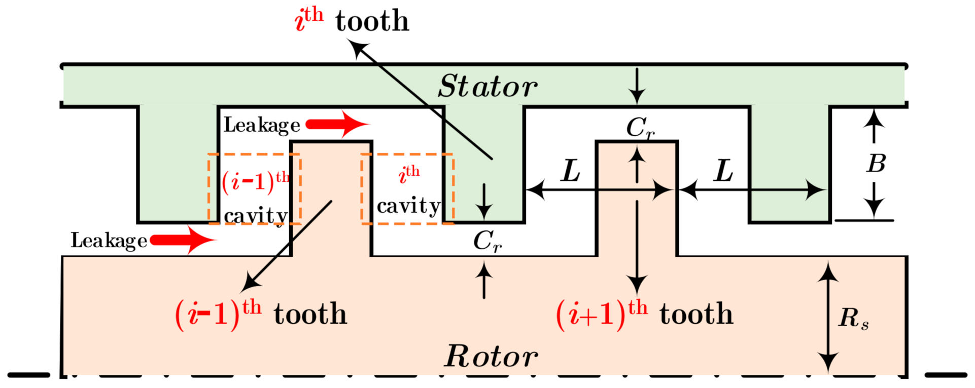
Two main types of labyrinth seals are applied in engineering practice, with one being the see-through style (including the seal teeth on the stator (TOS) and the seal teeth on the rotor (TOR)) and the other one being the interlocking style, which has its teeth both on the rotor and the stator (ILS). The ILS is considered in the present study, in which its geometry is illustrated in Figure 1. Detailed explanations regarding its dimensions can be found in Ref. [13].
In a typical cavity, the fluid dynamics are governed by the continuity equation and the circumferential momentum equation. When the concentric rotor rotates with a constant speed with no eccentricity, gas flow in the labyrinth seal is steady, axial-symmetric, and time-independent. Under this steady state, the continuity equation implies that the mass flow rate from one cavity to the next equals the constant m ˙ 0 , i.e.,
m ˙ 1 = = m ˙ i = = m ˙ N = m ˙ 0 , ( i = 1 , 2 , , N ) ,
where m ˙ i represents the mass flow rate through the clearance of the ith tooth. According to the generalized Neumann’s equation [1,13], the value of m ˙ i depends on the geometry, temperature, and pressure difference between two adjacent cavities, which can be written as
m ˙ i = m ˙ 0 = C 1 i C 2 i 2 π R s C r P i 1 2 P i 2 R g T i .
In Equation (2), the orifice contraction coefficient C 1 i is determined by Chaplygin’s formula [2,13]:
C 1 i = π π + 2 5 S i + 2 S i 2   with   S i = P i 1 P i ( γ 1 ) / γ 1 ,
where γ represents the specific heat ratio.
The kinetic energy carry-over coefficient C 2 i equals to unity for the first cavity, while
C 2 i = N ( 1 J i ) N + J i   with   J i = 1 1 + 16.6 C r L 2
gives its estimations for other teeth [2,13].
Geometric parameters in Equation (2) include the rotor radius Rs and the radial clearance Cr. The gas in each seal cavity is assumed to obey the ideal gas law. Thus, its pressure distribution can be written as
P i = ρ i R g T i ,
where ρ i , Rg, and Ti are the gas density, gas constant, and gas temperature, respectively. Usually, the isenthalpic flow results in an isothermal process for gas flows, which means a constant gas temperature is preserved among all the cavities ( T i = T , i = 1 , 2 , , N ).
Once the parameters in Equations (1)–(5) are provided, e.g., the gas temperature T, inlet pressure P in , and outlet pressure P out , the flow rate m ˙ i and pressure distribution P i in each cavity can be calculated by coupling these equations iteratively.
The randomness of the flow may generate randomly uncertain excitations, which will affect the stability and reliability of the seal-rotor system in practice. Thus, the randomly uncertain factors should be considered in establishing the circumference momentum equation [24], which is rewritten as
t ρ i V i d V ˜ + V i ρ i A d S = F θ + F r ( t ) ,
where V ˜ is the volume of each cavity and S is the surface of the control volume. Circumferential force F θ within the control volume of each cavity includes the pressure component and the shear force component, with both acting along the circumferential direction, while F r ( t ) represents the random excitation due to the uncertainty of the gas flow.
For the system shown in Figure 1, a specific form of Equation (6) is given by
ρ i A V i t + ρ i V i A R s V i θ + m ˙ i ( V i V i 1 ) = A R s P i θ + ( τ r i a r τ s i a s ) L + F r ( t ) R s H ,
where A = L ( B + H ) represents the cross-section area of a cavity and H is the non-asymmetric clearance. Both A and H vary with ( t , θ ) . The dimensionless shear stress lengths in Equation (7) are defined as
a r = a s = ( B + L ) / L .
For simplicity, we assume that the randomly uncertain perturbation is weak compared with the actions of the main gas flow, i.e.,
F r ( t ) = ε 0 f 0 ξ 0 ( t ) ,
where f0 is a constant and 0 ε 0 1 . The bounded noise excitation is expressed as [25]:
ξ 0 ( t ) = cos [ ω 0 t + σ B ( t ) + Γ ] ,
where ω 0 is the central frequency, B ( t ) is the standard Wiener process with strength σ , and Γ is a random phase uniformly distributed in the interval [ 0 , 2 π ) , which renders the process correlation-stationary at all times. The mean of the bounded noise is zero and
E ξ 0 ( t 1 ) ξ 0 ( t 2 ) = 1 2 cos ω 0 ( t 1 t 2 ) exp σ 2 2 t 1 t 2
gives the correlation function. Moreover, the two-sided spectral density of this random process can be computed as [25]
S ξ 0 ( Ψ ) = σ 2 2 π 1 4 ( Ψ ω 0 ) 2 + σ 4 + 1 4 ( Ψ + ω 0 ) 2 + σ 4 ,
and the shape of the power spectrum rests with ω 0 and σ . In general, it has two peaks symmetrically located in the positive and negative frequency domains. When ω 0 / σ 2 1 , ξ 0 ( t ) becomes a narrow-band random process, which provides a good simulation for the Dryden spectrum of wind turbulence and the von Karman spectrum of vibration transmitted through the ground by changing the values of ω 0 and σ [24].
Except for the pressures and velocities, many other parameters in the continuity equation and the circumferential momentum equation need to be determined. According to work by Eser [24], Equations (1) and (6) can be transformed by employing the perturbation method and neglecting the terms of order ε 2 and their higher-order counterparts as
G 1 P 1 i t + V 0 i R s P 1 i θ + P 0 i R s V 1 i θ + G 2 i P 1 i 1 + G 3 i P 1 i + G 4 i P 1 i + 1 = G 5 i H 1 t V 0 i R s H 1 θ
and
X 1 i V 1 i t + V 0 i R s V 1 i θ + A 0 R s P 1 i θ + X 2 i V 1 i m ˙ 0 V 1 i 1 + X 3 i P 1 i 1 + X 4 i P 1 i = X 5 i r H 1 .
The parameters involved in Equations (13) and (14) can refer to Ref. [24], except that the form of X 5 i r has now been changed to
X 5 i r = X 5 i + ε 0 f 0 ξ 0 ( t ) R s ,
where X 5 i has the same meaning as that in Ref. [24].
A new term ε 0 f 0 ξ 0 ( t ) / R s in Equation (15), resulting from the random uncertainties, will affect the estimations of the cavity parameters. To calculate the sealing force, most of the intermediate parameters embedded in these equations should be determined in advance, which can only be obtained with the orbit of the rotor center.

3. Estimations of the Dynamic Coefficients

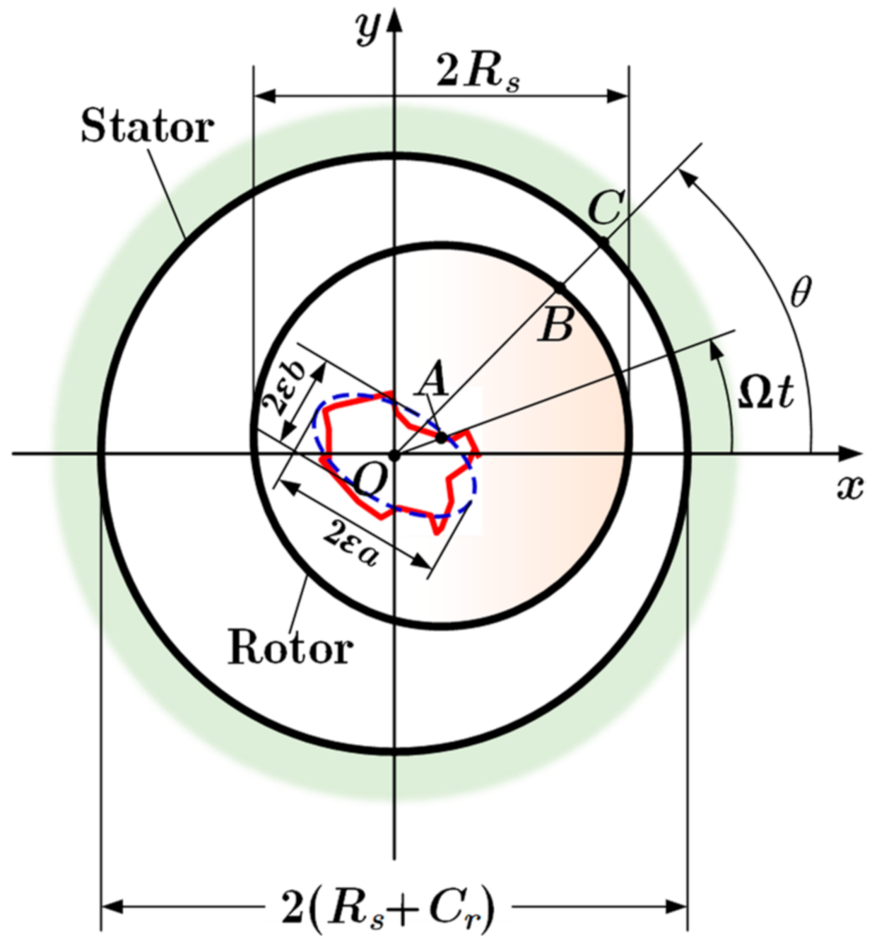
In the process of solving the first-order continuity equation and circumferential momentum equation, the orbit motion should be provided, which is primarily assumed to be a standard elliptic trajectory in the existing literature. However, random excitation from the uncertainty of gas flow causes the rotor center not to rotate along the elliptic trajectory. Therefore, taking the randomly uncertain factors into account, the horizontal and vertical position function of the rotor center A to cavity center O (see Figure 2) can be written as
x A = λ 1 cos Ω t + λ 2 sin Ω t + ε ξ x ( t ) y A = λ 3 sin Ω t + λ 4 cos Ω t + ε ξ y ( t ) ,
where
λ 1 λ 2 λ 3 λ 4 = K x x M C x x K x y C x y C x x K x x M C x y K x y K y x C y x K y y M C y y C y x K y x C y y K y y M 1 M ε 0 0 M ε .
Randomly uncertain perturbations in x- and y- directions can again be expressed by the bounded noises ξ x ( t ) and ξ y ( t ) . Assuming that the perturbations come from the same resources and have the same center frequency ω r but with different strengths ( σ x and σ y ) and random phases ( Γ x and Γ y ), their formation can be written as
ξ x ( t ) = f x cos ( ω r t + σ x B x ( t ) + Γ x ) ξ y ( t ) = f y cos ( ω r t + σ y B y ( t ) + Γ y ) .
According to Shinozuka’s work [26], each physical realization of the bounded noises can be generated by a series of cosine functions with random frequencies, i.e.,
ξ 0 ( t ) k = 1 N 0 Λ k cos ( ω k t + Γ k ) ,
where Λ k = 2 S ξ 0 Δ ω represents the amplitude, ω k is the non-negative random frequency independently distributed in the range [ ω l , ω u ] , Γ k is the random phase uniformly distributed in the interval [ 0 , 2 π ) , N0 is a positive integer with large enough value, and Δ ω = ( ω u ω l ) / N 0 is the frequency increment. As each physical realization of the bounded noises ξ 0 ( t ) is approximated by the sum of N0 harmonic functions, it can be considered a deterministic one. Physical realization from Equation (18) is almost ergodic for a large enough value of N0 [26].
Similarly, the physical realizations of ξ x ( t ) and ξ y ( t ) can be generated by
ξ x ( t ) g = 1 N 1 f x , g cos ( ω g t + Γ x , g ) ξ y ( t ) g = 1 N 1 f y , g cos ( ω g t + Γ y , g ) ,
where f x , g and f y , g are the amplitudes in the x- and y-directions, ω g is the non-negative independent random frequency, Γ x , g and Γ y , g are the random phases, and N1 is a positive integer with large enough value.
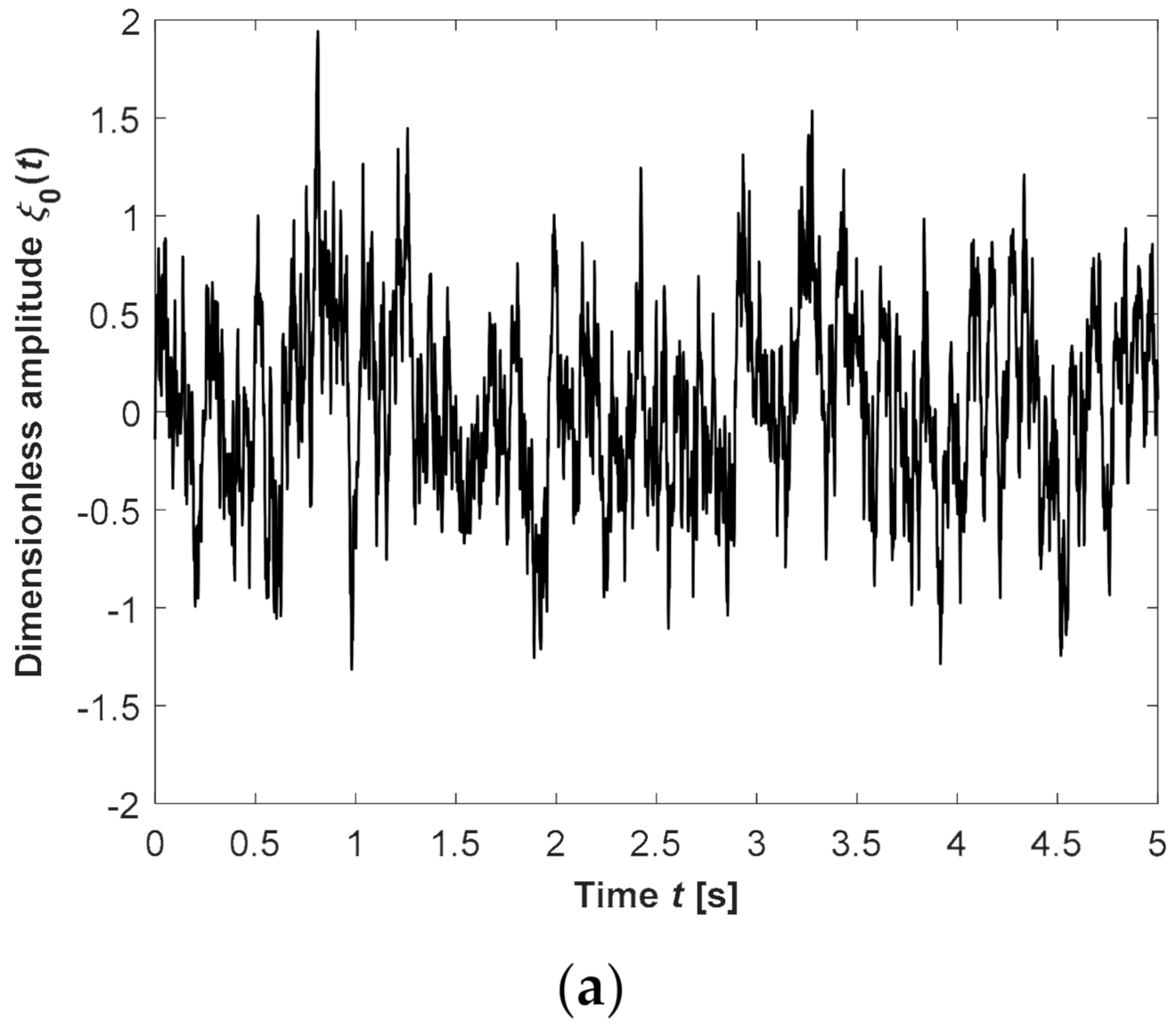
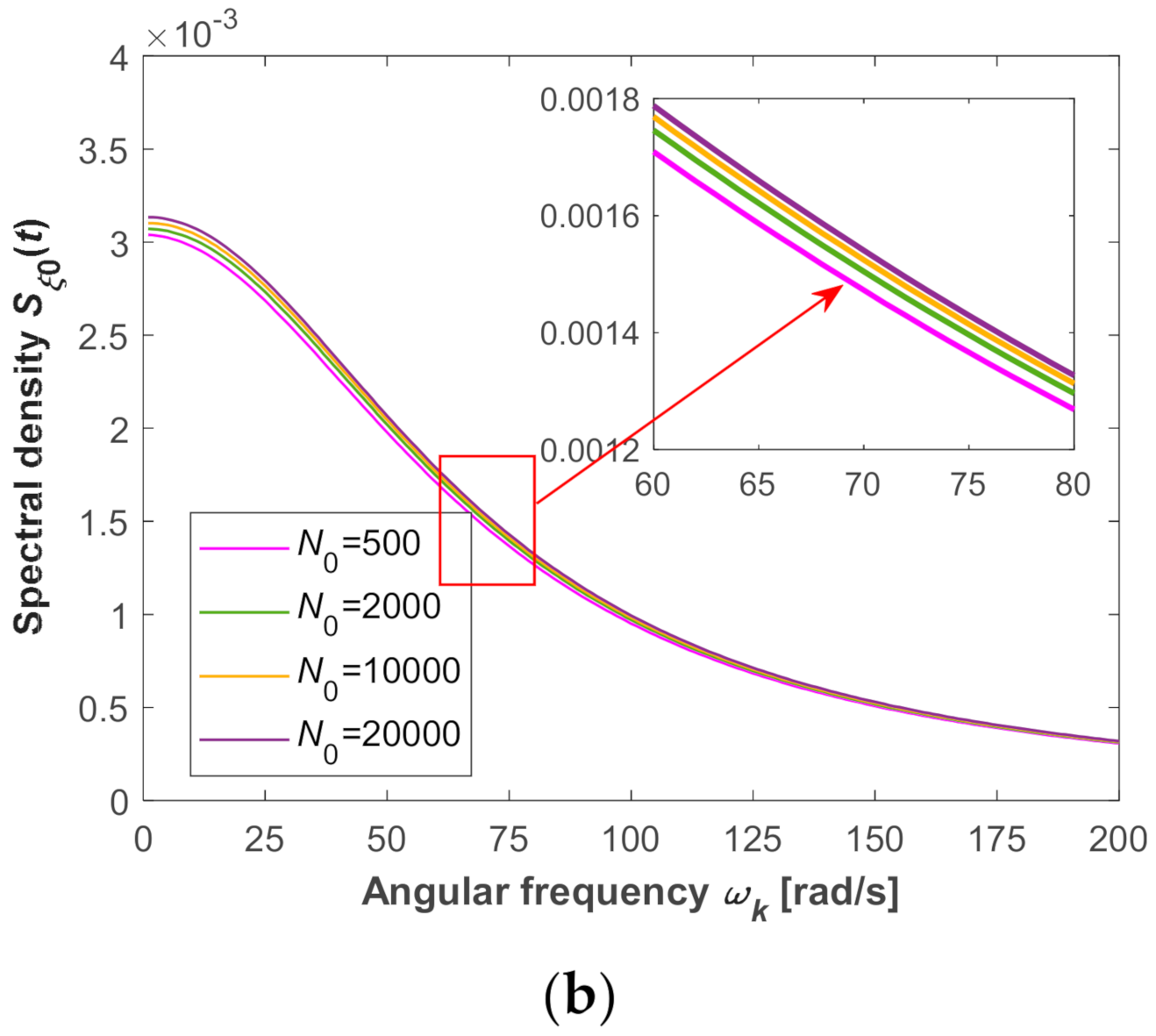
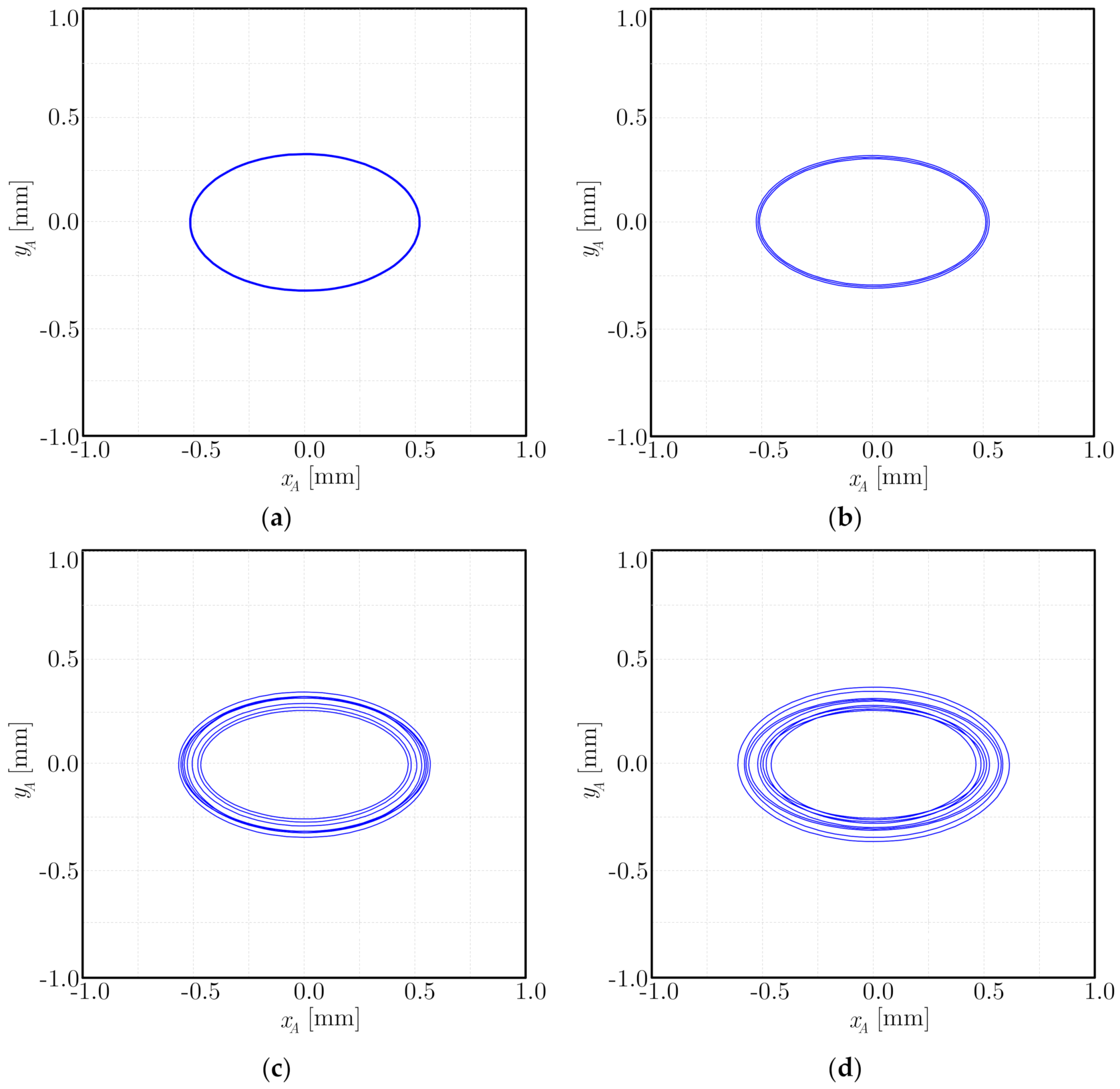
A sample function generated by Equation (18) is displayed in Figure 3a, where ω 0 = 2 π , σ = 10 , and N 0 = 2000 . When N0 approaches a large value, as shown in Figure 3b, its spectral density is almost consistent with the theoretical one, indicating that the sample function is a good approximation of random bounded noise and can ensure the ergodicity of each physical realization.
In Figure 2, the dashed ellipse is the idealized trajectory, while the solid red orbit represents its realistic counterpart with an uncertain bounded noise perturbation. The disturbance clearance function is defined by the distance between point B on the rotor and point C on the stator, written as
H ( t , θ ) = R s + C r O B ¯ .
As each sample of the bounded noise is simulated by a series of cosine functions, the perturbation analysis can be appreciably used to express the length of OB as
O B ¯ = R s ε H 1 ( t , θ ) + .
When the perturbation analysis is performed, the eccentricity of the disturbed rotor is characterized by the perturbation parameter ε = e / C r , where e is the deviation distance of the rotor center from the cavity center. The flow variables are then expanded as
H = C r + ε H 1 ( t , θ ) + P i = P 0 i + ε P 1 i ( t , θ ) + V i = V 0 i + ε V 1 i ( t , θ ) + q ˙ i = q ˙ 0 i + ε q ˙ 1 i ( t , θ ) + ρ i = ρ 0 i + ε ρ 1 i ( t , θ ) + τ r i = τ r 0 i + ε τ r 1 i ( t , θ ) + τ s i = τ s 0 i + ε τ s 1 i ( t , θ ) + .
Consequently, the coordinates of point B are derived as
x B = O B ¯ cos θ = R s cos θ ε H 1 ( t , θ ) cos θ + y B = O B ¯ sin θ = R s sin θ ε H 1 ( t , θ ) sin θ + .
Since A and B are located at the center and edge of the rotor, respectively, the distance between them equals to the radius Rs, i.e.,
( x B x A ) 2 + ( y B y A ) 2 = R s 2 .
Substituting Equations (16) and (22) into Equation (23), we can obtain that
R s cos θ ε H 1 ( t , θ ) cos θ ε a cos ( Ω t + φ A x ) ε ξ x ( t ) 2 + R s sin θ ε H 1 ( t , θ ) sin θ ε b sin ( Ω t + φ A y ) ε ξ y ( t ) 2 = R s 2 ,
where
a = λ 1 2 + λ 2 2 / ε b = λ 3 2 + λ 4 2 / ε   and   φ A x = arctan ( λ 2 / λ 1 ) φ A y = arctan ( λ 4 / λ 3 ) .
Neglecting the terms of ε 2 and the higher-order counterparts, H 1 ( t , θ ) can be derived as
H 1 ( t , θ ) = a cos Ω t + φ A x cos θ + b sin Ω t + φ A y sin θ ξ x ( t ) cos θ + ξ y ( t ) sin θ .
According to Equation (19), its exponential form is
H 1 ( t , θ ) = Re 1 2 a b e j θ + Ω t + φ A x + 1 2 a + b e j θ Ω t φ A y + g = 1 N 1 1 2 f x , g f y , g e j θ + ω g t + 1 2 f x , g + f y , g e j θ ω g t .
The solutions of the first-order continuity equation and momentum equation can be given by substituting Equation (26) into Equations (13) and (14) as
P 1 i = Re P i + e j θ + Ω t + φ A x + P i e j θ Ω t φ A y + g = 1 N 1 P i , g + e j θ + ω g t + P i , g e j θ ω g t ,
V 1 i = Re V i + e j θ + Ω t + φ A x + V i e j j θ Ω t φ A y + g = 1 N 1 V i , g + e j θ + ω g t + V i , g e j θ ω g t .
where the parameters P i + , P i , g + , V i + , and V i , g + with the superscript ‘+’ represent the coefficients of the terms e j ( θ + Ω t + φ A x ) and e j ( θ + ω g t ) , while the parameters P i , P i , g , V i , and V i , g with the superscript ‘ ’ represent the coefficients of the terms e j ( θ Ω t φ A y ) and e j ( θ ω g t ) .
It can be found from the expressions of H 1 , P 1 i , and V 1 i that the intermediate parameters are comprised of two parts under the uncertain perturbations. The former part corresponds to the ideal elliptic orbit, and the second part corresponds to the fluctuation caused by the weak bounded noise. During a certain iteration process, the fluctuations of the intermediate parameters are different from each other among the various samples.
Substituting Equations (26)–(28) into Equations (13) and (14) yields
j G 1 V 0 i R s ± Ω P i ± + P 0 i R s V i ± + G 2 i P i 1 ± + G 3 i P i ± + G 4 i P i + 1 ± = j G 5 i a ± b 2 Ω V 0 i R s ,
j X 1 i V 0 i R s ± Ω V i ± + j A 0 R s P i ± + X 2 i V i ± m ˙ 0 V i 1 ± + X 3 i P i 1 ± + X 4 i P i ± = X 5 i + ε 0 f 0 R s k = 1 N 0 Λ k cos ω k + Γ k a b 2 ,
g = 1 N g j G 1 V 0 i R s ± ω g P i , g ± + P 0 i R s V i , g ± + G 2 i P i 1 , g ± + G 3 i P i , g ± + G 4 i P i + 1 , g ± = j G 5 i g = 1 N 1 ω g V 0 i R s f x , g ± f y , g 2 ,
and
g = 1 N g j X 1 i ( V 0 i R s ± ω g ) V i , g ± + j A 0 R s P i , g ± + X 2 i V i , g ± m ˙ 0 V i 1 , g ± + X 3 i P i 1 , g ± + X 4 i P i , g ± , = X 5 i + ε 0 f 0 R s k = 1 N 0 Λ k cos ω k + Γ k g = 1 N 1 f x , g f y , g 2
where the parameters with a subscript ‘g’ represent the fluctuation components due to the bounded noise.
In previous studies, only Equations (29) and (30) were investigated, and the additional term ( ε 0 f 0 / R s ) k = 1 N 0 ( Λ k cos ω k + Γ k ) in Equation (30) was not included. Equations (31) and (32) are introduced here due to the random uncertainty in the orbit motion. Obviously, compared with the traditional ellipse case, more parameters and additional equations are involved during the solution process. For the convenience of analysis, we define the vectors as follows:
Y i = P i + , P i , V i + , V i T ,
Z i = P i , g + , P i , g , V i , g + , V i , g T ,
and Equations (29)–(32) can be transformed into their matrix forms as
C i 1 Y i 1 + C i 0 Y i + C i + 1 Y i + 1 = A i ,
C ^ i 1 Z i 1 + C i 0 Z i + C i + 1 Z i + 1 = A ^ i ,
where
C i 1 = j G 1 V 0 i R s + Ω + G 3 i 0 j G 1 P 0 i R s 0 0 j G 1 V 0 i R s Ω + G 3 i 0 j G 1 P 0 i R s j A 0 R s + X 4 i 0 j X 1 i V 0 i R s + Ω + X 2 i 0 0 j A 0 R s + X 4 i 0 j X 1 i V 0 i R s Ω + X 2 i ,
C ^ i 1 = j G 1 V 0 i R s + g = 1 N 1 ω g + G 3 i 0 j G 1 P 0 i R s 0 0 j G 1 V 0 i R s g = 1 N 1 ω g + G 3 i 0 j G 1 P 0 i R s j A 0 R s + X 4 i 0 j X 1 i V 0 i R s + g = 1 N 1 ω g + X 2 i 0 0 j A 0 R s + X 4 i 0 j X 1 i V 0 i R s g = 1 N 1 ω g + X 2 i ,
C i 0 = G 2 i 0 0 0 0 G 2 i 0 0 X 3 i 0 m ˙ 0 0 0 X 3 i 0 m ˙ 0 ,
C i + 1 = G 4 i 0 0 0 0 G 4 i 0 0 0 0 0 0 0 0 0 0 ,
A i = j G 5 i a b 2 Ω V 0 i R s , j G 5 i a + b 2 Ω + V 0 i R s , X 5 i + ε 0 f 0 R s k = 1 N 0 Λ k cos ω k + Γ k a b 2 , X 5 i + ε 0 f 0 R s k = 1 N 0 Λ k cos ω k + Γ k a + b 2 T ,
and
A ^ i = j G 5 i g = 1 N 1 f x , g f y , g 2 ω g V 0 i R s , j G 5 i g = 1 N 1 f x , g + f y , g 2 ω g + V 0 i R s , X 5 i + ε 0 f 0 R s k = 1 N 0 Λ k cos ω k + Γ k g = 1 N 1 f x , g f y , g 2 , X 5 i + ε 0 f 0 R s k = 1 N 0 Λ k cos ω k + Γ k g = 1 N 1 f x , g + f y , g 2 ] T .
Equations (33)–(36) involve twelve unknown parameters, including P i + , P i , V i + , and V i for the ith cavity and their counterparts for the ( i 1 ) th and ( i + 1 ) th cavity. Besides, an extra series of randomly uncertain parameters P i , g + , P i , g , V i , g + , and   V i , g is also included. Considering a labyrinth seal with ( N 1 ) cavities, a system of four linear equations can be written for each cavity as
C i 1 1 C i 1 0 C i 1 + 1 0 0 0 C i 1 C i 0 C i + 1 0 0 0 C i + 1 1 C i + 1 0 C i + 1 + 1 Y i 1 Y i Y i + 1 = A i 1 A i A i + 1 ,
C ^ i 1 1 C i 1 0 C i 1 + 1 0 0 0 C ^ i 1 C i 0 C i + 1 0 0 0 C ^ i + 1 1 C i + 1 0 C i + 1 + 1 Z i 1 Z i Z i + 1 = A ^ i 1 A ^ i A ^ i + 1 ,
resulting in an 8 ( N 1 ) × 8 ( N 1 ) banded system with linear equations to determine the unknowns. The above equations can be solved by applying the Gaussian elimination method.
Since asymmetric forces exist during operation, rotor performances characterized by the direct and cross-coupled stiffness and damping coefficients should be changed accordingly. The equation of motion of the seal-rotor system can then be written as [24]:
C x x C x y C y x C y y x ˙ y ˙ + K x x K x y K y x K y y x y = F x F y ,
where Fx and Fy are the total net forces generated by the gas leakage in x- and y-directions, respectively. The influence coefficients in the damping and stiffness matrix satisfy C x x = C y y , C x y = C y x , K x x = K y y , and K x y = K y x . It should be noted that the coefficients in Equation (45) originate only from one sample of the randomly uncertain trials, and 32 or more samples are required to ensure ergodicity.
The total net forces can be obtained by integrating the disturbance pressure and disturbance shear stress along the rotor surface as follows:
F = F x + j F y = ε R s L i = 1 N 0 2 π P 1 i e j θ j 1 + B L τ r 1 i e j θ d θ .
Substituting the pressure component, the shear force component, and the intermediate parameters into Equation (46), we obtain that,
F = 2 π ε R s L i = 1 N P ¯ i 1 j 1 + B L τ r 0 i P 0 i j 1 + B L 1.75 τ r 0 i V 0 i ω R s V ¯ i + 0.125 τ r 0 i D h 0 ( B + C r ) 2 a + b 2 e j Ω t + φ A x + P ¯ i + 1 j 1 + B L τ r 0 i P 0 i j 1 + B L 1.75 τ r 0 i V 0 i ω R s V ¯ i + + 0.125 τ r 0 i D h 0 ( B + C r ) 2 a b 2 e j Ω t + φ A y + g = 1 N 1 P ¯ i , g 1 j 1 + B L τ r 0 i P 0 i j 1 + B L 1.75 τ r 0 i V 0 i ω R s V ¯ i , g + 0.125 τ r 0 i D h 0 ( B + C r ) 2 f x , g + f y , g 2 e j ω g t + g = 1 N 1 P ¯ i , g + 1 j 1 + B L τ r 0 i P 0 i j 1 + B L 1.75 τ r 0 i V 0 i ω R s V ¯ i , g + + 0.125 τ r 0 i D h 0 ( B + C r ) 2 f x , g f y , g 2 e j ω g t ,
where the randomly uncertain factors caused by the gas excitation is also included. Similarly, substituting the randomly uncertain orbit expression Equation (19) into Equation (45), the total net forces can be written as.
F = F x + j F y = ε 2 K x x + C x y Ω j K x y C x x Ω a + b e j Ω t + φ A x K x x C x y Ω j K x y + C x x Ω a b e j Ω t + φ A y + g = 1 N 1 K x x + C x y ω g j K x y C x x ω g f x , g + f y , g e j ω g t + g = 1 N 1 K x x C x y ω g j K x y + C x x ω g f x , g f y , g e j ω g t .
Comparing Equation (48) with Equation (47) by defining
M + = π R s L i = 1 N P ¯ i + 1 j 1 + B L τ r 0 i P 0 i j 1 + B L 1.75 τ r 0 i V 0 i ω R s V ¯ i + + 0.125 τ r 0 i D h 0 B + C r 2 a + b 2 2 a + b ,
M = π R s L i = 1 N P ¯ i 1 j 1 + B L τ r 0 i P 0 i j 1 + B L 1.75 τ r 0 i V 0 i ω R s V ¯ i + 0.125 τ r 0 i D h 0 B + C r 2 a b 2 2 a b ,
N + = π R s L i = 1 N g = 1 N 1 P ¯ i , g + 1 j 1 + B L τ r 0 i P 0 i j 1 + B L 1.75 τ r 0 i V 0 i ω R s V ¯ i , g + + 0.125 τ r 0 i D h 0 B + C r 2 f x , g + f y , g 2 2 f x , g + f y , g ,
and
N = π R s L i = 1 N g = 1 N 1 P ¯ i , g 1 j 1 + B L τ r 0 i P 0 i j 1 + B L 1.75 τ r 0 i V 0 i ω R s V ¯ i , g + 0.125 τ r 0 i D h 0 B + C r 2 f x , g f y , g 2 2 f x , g f y , g ,
the dynamic coefficients are derived as
K x x = 1 2 Re M + + M + N + + N K x y = 1 2 Im M + + M + N + + N C x x = 1 2 Ω Im M + M + N + N C x y = 1 2 Ω Re M + M + N + N .
As previously mentioned, the external random excitation will disturb the gas flow in a labyrinth seal, and in return, the variation of the gas flow brings about an unstable sealing force acting on the rotor to cause further unpredictable variations of the rotor position. The parameters of each cavity, such as P i ± and V i ± , will change with the random excitation, which can directly affect the values of M ± and N ± . Therefore, all the above factors are closely linked with each other during the calculation process, and the dynamic coefficients will deviate from the ideal ones, which can be seen from Equation (53).
Although each sample of a random process can be recognized as a deterministic realization once it is generated by some approximation method, even faint noisy factors may bring about obvious change and affect the stability of the rotor system. To show the impact of random uncertainty on the dynamic coefficients, several numerical examples are illustrated in the following section for a more detailed discussion of the results.

4. Illustrating Examples

Unless otherwise indicated, the geometry parameters and working conditions applied for the simulations of the presented system are all listed in Table 1. Assume that an airflow exists in the ILS, and the geometric parameters remain unchanged in the axial direction.
The dynamic coefficients are calculated for the elliptic orbits with and without randomly uncertain perturbation. Therefore, we define a proportional coefficient as δ F = F r ( t ) / F θ to control the strength of the bounded noise among all of the simulations. Similarly, another proportional coefficient is defined as δ R = f x / a = f y / b for the randomly uncertain perturbation on the orbit motion. Since the orbit fluctuation results from the random excitation of the airflow, we discuss the specific case as δ F = δ R , while similar analysis can be performed for other cases.

4.1. Calculation of the Orbit Motion

As mentioned in Section 1, the randomly uncertain perturbation in the gas flow will result in random excitation acting on the rotor, and the sealing force calculated by Equation (47) is unstable due to the random excitation and the fluctuation of parameters of each cavity. In the present work, the proposed nonparametric method is employed to show the effects of randomly uncertain factors on the sealing force, see Figure 4, where the coefficient δ R is set to be 0 (ideal state), 0.02, 0.08, and 0.20 for comparison. To be noticed is that the sudden phase shifts shown in 10.05, 10.1, and 10.15 sec result from ωg (see Equation (47)), which is a non-negative random frequency independently distributed in a certain range (see Equation (19)) and is used to periodically control the rhythm of a stochastic process. Besides, the different amplitude fluctuations shown in the figures are controlled by fx,g and fy,g, which are determined by the coefficient δ R .
It can be seen from Figure 4 that the variation pattern of the sealing force for all three randomly uncertain cases has small differences to that of the ideal state. However, as δ R increases, the fluctuation of the peak values is becoming gradually stronger, resulting in stronger randomness of the orbit motion. Correspondingly, the orbit motion is no longer a regular ellipse but fluctuates with the random excitation.
The orbit shown in Figure 5 is not obtained directly from Equation (16) but is calculated by substituting the results from the dynamic coefficients and the sealing forces into Equation (45). This calculation process objectively describes the effect of random uncertainty.
It is easy to infer from Equation (16) that the orbit motion under random noise excitation should be an ellipse with fluctuations, which follows the analysis of M ± and N ± affected by the random excitation in Equation (53), see Figure 5b–d. Furthermore, another obvious phenomenon is that the orbit fluctuation becomes increasingly stronger as δ R increases, which is consistent with the previous analysis.

4.2. Parameter Influences on the Dynamic Coefficients

The influence of the rotating speed, pressure difference, and whirl velocity on the dynamic coefficients are extensively discussed in the following content. In total, 32 samples are generated for each case of random uncertainty to ensure the ergodicity of the results. The statistical properties from these samples are also compared with the deterministic ones from the ideal elliptic orbit. Besides, the samples from a certain simulation trial are also listed for the comparisons with the statistical and theoretical results.
Dynamic coefficients under the three cases δ R = 0.02 , 0.08 , and   0.20 are given in Figure 6, Figure 7 and Figure 8 for several values of the rotating speed, pressure difference, and inlet whirl velocity, respectively. It shows that the coefficients under the three cases deviate to some extent from the theoretical ones, which are the combined effects of the random excitation term in Equation (30) and the randomly uncertain perturbation of the orbit motion in Equation (16). It also can be seen that the deviation level is directly related to the intensity of the random uncertainty, which is consistent with the results obtained in the previous subsection.
More specifically, for each value of δ R , the four dynamic coefficients show completely different variation patterns as the rotating speed increases. Figure 6a shows that Kxx increases monotonically as the rotating speed increases. Simultaneously, its deviation levels from the theoretical values remain unchanged through the whole speed range. In Figure 6b, although Kxy basically decreases with the rotating speed, its deviation level under the case δ 0.20 max shows a large fluctuation at 6000–10,500 rpm, making Kxy slightly increase in this speed range. As for the damping coefficient, the envelopes of Cxx in Figure 6c show a downward trend against the rotating speed, whereas the deviation under the case δ 0.20 max only illustrates some smaller negative slopes at 6000–9000 rpm, not affecting the monotonicity of the envelope. Figure 6d depicts a monotonically increasing Cxy whose deviations from the theoretical value gradually shrink. Besides the envelope trends, the deviation levels from their corresponding theoretical values are positively related to the random uncertainty intensity. For the samples on the other side, their values may illustrate significant fluctuations from the theoretical ones, e.g., Kxx and Cxy. Considering that the intensity of random uncertainty in each of the three cases is relatively weak compared to the airflow and that the operating conditions are even more complex in practice, great difficulties will undoubtedly be encountered in estimating these coefficients.
Figure 7 shows the trends of the four coefficients over the pressure difference between the inlet and outlet pressures. Obvious changes appear for the first three coefficients Kxx, Kxy, and Cxx among the various pressure differences, indicating that pressure difference is one of the main parameters affecting the dynamic coefficients. Figure 7a,b display an opposite trend for the two stiffness coefficients. A monotonically increased Kxx and a monotonically decreased Kxy are observed for an enlarged pressure difference. On the other hand, the two damping coefficients under the various pressure differences also have distinct envelope trends. Cxx in Figure 7c shows a remarkable reduction, while Cxy in Figure 7d remains almost unchanged. For all of the four coefficients, their deviation levels remain unchanged and are positively correlated with the intensity of random uncertainty, regardless of the pressure difference. Unlike the statistical results of the 32 samples, the envelope of a single sample exhibits large fluctuations, e.g., Kxx and Cxy.
Variations of the four coefficients against the inlet whirl velocity are illustrated in Figure 8, in which the monotonically increasing Kxx (see Figure 8a) and the decreasing Kxy, Cxx, and Cxy (see Figure 8b–d) are observed for a larger inlet whirl velocity. It is worth noting that Kxy and Cxx go through a short period of increase (see the inlet whirl velocity range 10–20 m/s for δ 0.20 max in Figure 8b,c) before decreasing monotonically (corresponding to the inlet whirl velocity range 20–50 m/s for δ 0.20 max in Figure 8b,c). Simultaneously, the values of Kxx and Cxy for the single sample case fluctuate greatly due to the changes in inlet whirl velocity and the stochastic nature of a certain trial simulation. However, the fluctuations are smoothed as the number of sample cases becomes larger. Besides the envelope trends, the deviation levels of Kxx and Cxy remain unchanged throughout the velocity range, and those of Kxy and Cxx slightly shrink for a larger inlet whirl velocity. Moreover, the larger the intensity of the random uncertainty for the inlet whirl velocity, the larger the deviation levels are, as shown by the envelopes of Kxx and Cxy under different randomly uncertain factors δ R .
From Figure 6, Figure 7 and Figure 8, we found that the influence of pressure difference on Cxy (see Figure 7d) and that of inlet whirl velocity on Kxx (see Figure 8a) are considerably mild, but the randomly uncertain factors can bring a higher deviation level of the two coefficients. On the other hand, the four dynamic coefficients turn out to be sensitive to the change in rotating speed, and the effect of randomly uncertain factors may be concealed to some extent (see Cxy in Figure 6d, for example). As for the effects of pressure difference and inlet whirl velocity on the four coefficients, each coefficient shows completely different responses, see Kxy in Figure 7b and Figure 8b and Cxx in Figure 7c and Figure 8c. Moreover, the effects of the randomly uncertain factors on Kxx and Cxy exhibit stronger deviations than those on Kxy and Cxx.
Indeed, random excitation effects on the rotor and randomly uncertain perturbation on the orbit motion interrelate with each other. Thus, it is reasonable to consider the coupled influence of the two kinds of random uncertainty. From the analysis in Section 3 and the results shown in Figure 6, Figure 7 and Figure 8, it is inferred that the coupled influence sometimes enlarges the deviations but may reduce them at other times. In brief, the random uncertainty effect on dynamic coefficients is obvious, and if trials are made to ignore its role, large errors will undoubtedly occur.

5. Conclusions

In field applications, random uncertainties (e.g., turbulent gas flow, nonuniform gas flow forces, multi-direction spiral flow, and leakage) inevitably exist when gas flows through the labyrinth seal, causing random excitations to be generated and irregular deviations of the orbit motion from an elliptic trajectory. From this point of view, the rotordynamic coefficients of a seal-rotor system are investigated in our work by adopting the random uncertainty method and are rederived sequentially by adding the corresponding stochastic terms into the solving model. The orbit of the rotor center is assumed to be made up of two parts, i.e., a regular ellipse and a bounded noise perturbation, from which the disturbance clearance function, the corresponding coefficients of each cavity, and the sealing force acting on the rotor are rederived. Through the random uncertainty modeling technique, not only can the experimental deviations of dynamic coefficients be proved by the statistical analysis results of their theoretical values, but rules can also be made to guide the field design works rather than relying on some theoretical results from the deterministic models.
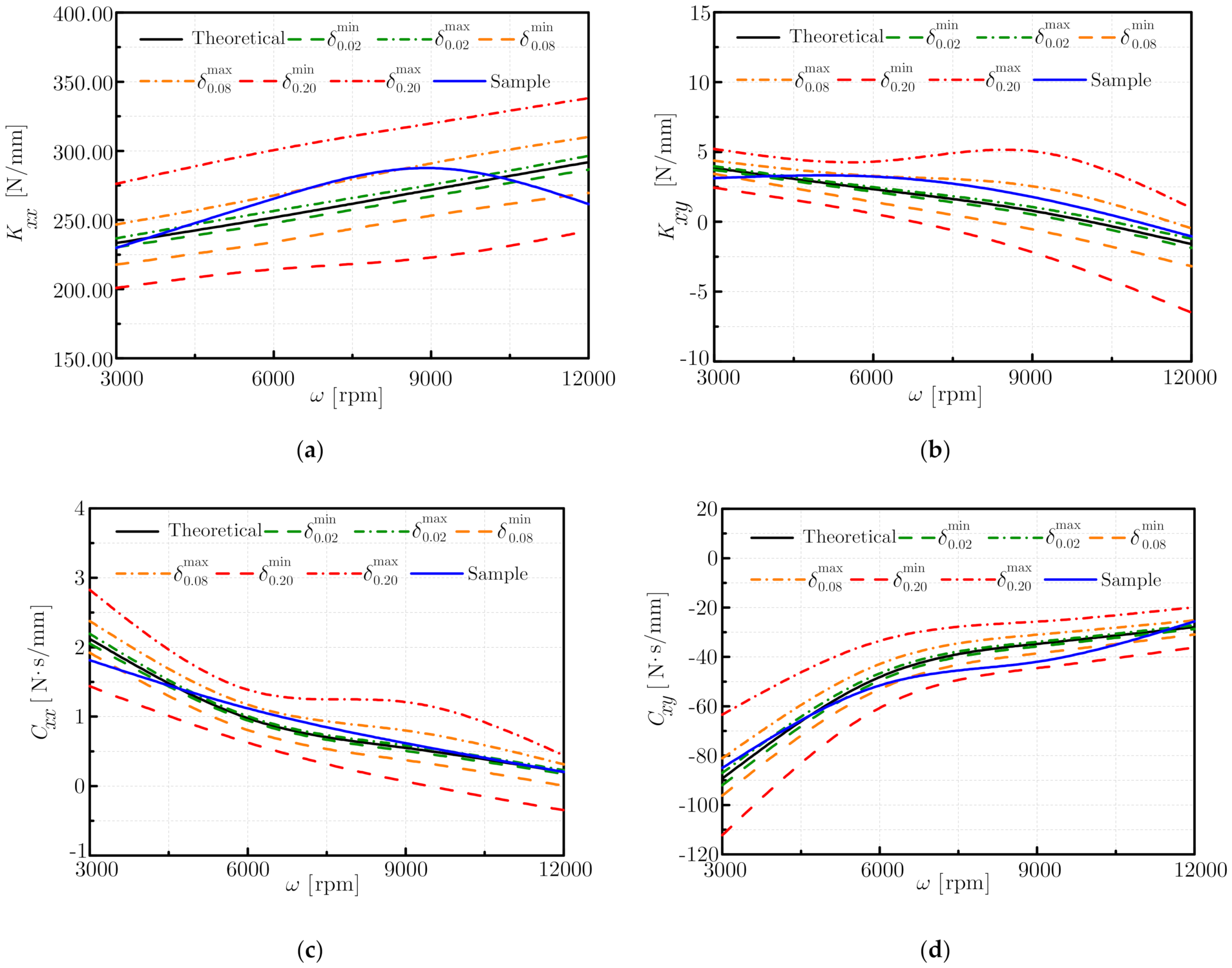
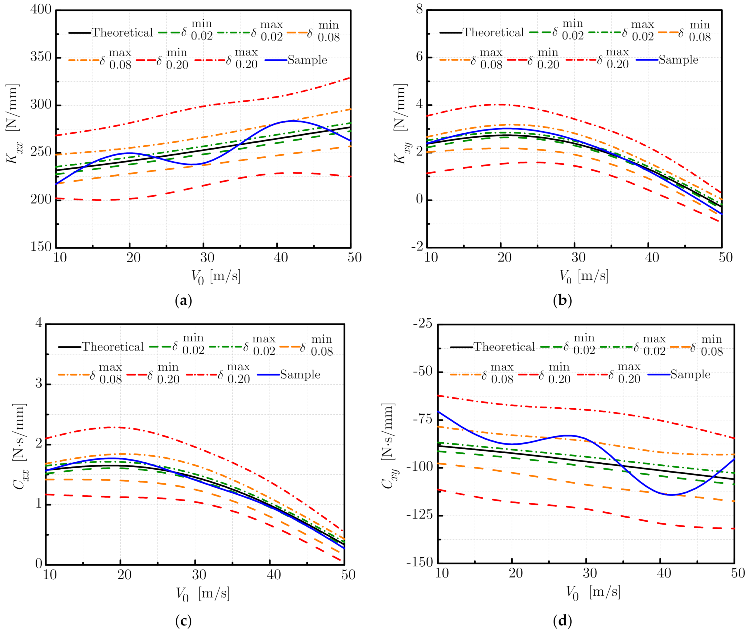
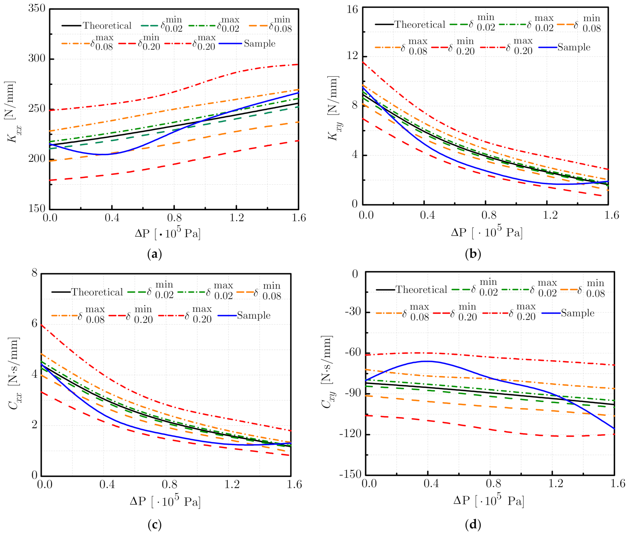
In total, 32 samples of the randomly uncertain orbit are generated for different rotating speeds, pressure differences, and inlet whirl velocities. The orbits are compared with their theoretical ones corresponding to the regular elliptic orbits. Numerical results show that differences exist among the effects of rotating speed, pressure difference, and inlet whirl velocity. Generally speaking, strong deviations in the direct stiffness and cross-coupled damping coefficients arise under the randomly uncertain factors. More specifically, Kxx monotonically increases and Kxy decreases as the rotating speed increases. The envelopes of Cxx show a downward trend, and Cxy monotonically increases against the rotating speed. Pressure difference also significantly affects the dynamic coefficients. A monotonically increased Kxx and a decreased Kxy are observed for an enlarged pressure difference. On the other hand, Cxx shows a remarkable reduction while Cxy remains almost unchanged. As for the inlet whirl velocity, a monotonically increasing Kxx and a decreasing Kxy, Cxx, and Cxy are observed for a larger inlet whirl velocity. To be noted is that Kxy and Cxx go through a short period of increase before decreasing monotonically. Deviation levels of the dynamic coefficients are directly related to randomly uncertain perturbations and are usually positively related to such perturbation strengths.
Thus, the running status of the rotor cannot be accurately revealed by the previous models under ideal conditions. It is necessary to take the uncertain factors into consideration to have an insight into the system behavior. We believe that the present work can help others to study the effects of uncertain factors on the dynamic coefficients of large rotating machinery from a practical point of view.

Author Contributions

Data curation, Y.Z. and Y.W.; Investigation, X.X. All authors have read and agreed to the published version of the manuscript.

Funding

This research was funded by the National Natural Science Foundation of China, under grant number 52075311, and the Science and Technology Innovation Action Plan of Shanghai, under grant number 21SQBS01400.

Institutional Review Board Statement

Not applicable.

Informed Consent Statement

Not applicable.

Data Availability Statement

Not applicable.

Conflicts of Interest

The authors declare no conflict of interest.

Nomenclature

AUnsteady cross-sectional area of the cavityRgGas constant
BTooth heightTGas temperature
C1iOrifice contraction coefficient of the ith cavityVi, V0i, V1iUnsteady/steady/perturbed tangential velocity in the ith cavity
C2iKinetic energy carry-over coefficient of the ith cavityar, asDimensionless length of the rotor and stator
CrSteady radial clearancea, bMajor/minor semiaxis of elliptical orbit motion
Cxx, CyyDirect damping coefficients in x- and y-directioneDeviation distance of the rotor center
Cxy, CyxCross-coupled damping coefficients in x- and y-directionf0Amplitude of the random excitation
Dh, Dh0Unsteady/steady hydraulic diameter of the cross-sectional area of the cavityfx, fyRandomness of the amplitude of the orbit in x- and y-direction
FTotal reaction force acting on the rotor m ˙ i, m ˙ 0Unsteady/steady mass flow rate in the ith orifice
Fx, FyComponent forces in x- and y- directionqi, q0i, q1iUnsteady/steady/perturbed leakage flow rate per unit length in the ith cavity
FrRandom excitationΓRandom phase of the bounded noise
FθCircumferential forceΩRotor whirling speed
H, H1Unsteady/perturbed radial clearanceδProportional coefficient to control the strength of the bounded noise
Kxx, KyyDirect stiffness coefficients in x- and y-directionεPerturbed parameter normalized by steady radial clearance
Kxy, KyxCross-coupled stiffness coefficients in x- and y-directionθAzimuthal position
LCavity lengthξBounded noise
NTooth numberρi, ρ0i, ρ1iUnsteady/steady/perturbed gas density of the ith cavity
Pi, P0i, P1iUnsteady/steady/perturbed pressure in the ith cavityτri, τr0i, τr1iUnsteady/steady shear stresses of the ith cavity at the rotor wall
Pin, PoutInlet/outlet pressureτsi, τs0i, τs1iUnsteady/steady/perturbed shear stresses of the ith cavity at the stator wall
RsRotor radiusωRotor rotating speed

References

  1. Childs, D. Turbomachinery Rotordynamics—Phenomena, Modeling and Analysis; John Wiley & Sons: New York, NY, USA, 1993. [Google Scholar]
  2. Cangioli, F.; Pennacchi, P.; Vannini, G.; Ciuchicchi, L. Effect of energy equation in one control-volume bulk-flow model for the prediction of labyrinth seal dynamic coefficients. Mech. Syst. Signal. Process. 2018, 98, 594–612. [Google Scholar] [CrossRef]
  3. Zhang, W.; Gu, Q.; Wang, T. Study on the rotordynamic performance of a novel anti-stagnation labyrinth seal. J. Vib. Eng. Technol. 2020, 8, 835–846. [Google Scholar] [CrossRef]
  4. Zhang, W.; Gu, Q.; Cao, H.; Wang, Y.; Yin, L. Improving the rotordynamic stability of short labyrinth seals using positive preswirl. J. Vibroeng. 2020, 22, 1295–1308. [Google Scholar] [CrossRef]
  5. Zhang, W.; Wu, K.; Gu, C.; Tian, H.; Zhang, X.; Li, C. Swirl brakes optimization for rotordynamic performance improvement of labyrinth seals using computational fluid dynamics method. Tribol. Int. 2021, 159, 106990. [Google Scholar] [CrossRef]
  6. Chen, Y.; Li, Z.; Li, J.; Yan, X. Effects of swirl brake axial arrangement on the leakage performance and rotor stability of labyrinth seals. Chin. J. Aeronaut. 2021, 34, 22–31. [Google Scholar] [CrossRef]
  7. Jiang, J.; Yang, Y.; Li, Y.; Huang, W. Theoretical and experimental investigation on maximum pressure loads of labyrinth seal’s teeth. Adv. Mech. Eng. 2018, 10, 1687814018794348. [Google Scholar] [CrossRef] [Green Version]
  8. Mo, J.; Yu, Z.; Luo, Y.; Du, H. Numerical and experimental analysis of the rotor eccentric effect on the labyrinth seal. In IOP Conference Series: Materials Science and Engineering, Proceedings of the 6th International Conference on Mechanical, Materials and Manufacturing, Boston, USA, 12–14 October 2019; IOP Publishing: Bristol, UK, 2019; Volume 689, p. 012012. [Google Scholar]
  9. Jia, X.; Zhang, H.; Zheng, Q.; Fan, S.; Tian, Z. Investigation on rotor-labyrinth seal system with variable rotating speed. Int. J. Turbo. Jet. Eng. 2019, 36, 19–29. [Google Scholar] [CrossRef]
  10. Chen, Y.; Li, Z.; Li, J.; Yan, X. Effects of tooth bending damage on the leakage performance and rotordynamic coefficients of labyrinth seals. Chin. J. Aeronaut. 2020, 33, 1206–1217. [Google Scholar] [CrossRef]
  11. Cangioli, F.; Chatterton, S.; Pennacchi, P.; Nettis, L.; Ciuchicchi, L. Thermo-elasto bulk-flow model for labyrinth seals in steam turbines. Tribol. Int. 2018, 119, 359–371. [Google Scholar] [CrossRef]
  12. Pugachev, A.; Gaszner, M.; Georgakis, C.; Cooper, P. Segmentation effects on brush seal leakage and rotordynamic coefficients. J. Eng. Gas. Turbines. Power 2016, 138, 032501. [Google Scholar] [CrossRef]
  13. Wu, T.; Andrés, L. Gas labyrinth seals: On the effect of clearance and operating conditions on wall friction factors—A CFD investigation. Tribol. Int. 2019, 131, 363–376. [Google Scholar] [CrossRef]
  14. Zhang, M.; Yang, J. Spiral flow induced destabilizing force analysis and its reduction with a novel helix-comb gas seal. Aerosp. Sci. Technol. 2020, 105, 105997. [Google Scholar] [CrossRef]
  15. Ma, H.; Li, H.; Niu, H.; Song, R.; Wen, B. Nonlinear dynamic analysis of a rotor-bearing-seal system under two loading conditions. J. Sound. Vib. 2013, 332, 6128–6154. [Google Scholar] [CrossRef]
  16. Nembhard, A.; Sinha, J.; Yunusa-Kaltungo, A. Experimental observations in the shaft orbits of relatively flexible machines with different rotor related faults. Measurement 2015, 75, 320–337. [Google Scholar] [CrossRef]
  17. Zhang, E.; Jiao, Y.; Chen, Z. Dynamic behavior analysis of a rotor system based on a nonlinear labyrinth-seal forces model. J. Comput. Nonlinear. Dyn. 2018, 13, 101002. [Google Scholar] [CrossRef]
  18. Yan, X.; He, K.; Li, J.; Feng, Z. Numerical techniques for computing nonlinear dynamic characteristic of rotor-seal system. J. Mech. Sci. Technol. 2014, 28, 1727–1740. [Google Scholar] [CrossRef]
  19. Xu, Q.; Niu, J.; Yao, H.; Zhao, L.; Wen, B. Nonlinear dynamic behavior and stability of a rotor/seal system with the dynamic vibration absorber. Adv. Mech. Eng. 2019, 11. [Google Scholar] [CrossRef] [Green Version]
  20. Zahorulko, A.; Lee, Y. Computational analysis for scallop seals with sickle grooves, Part II: Rotordynamic characteristics. Mech. Syst. Signal. Process. 2021, 147, 107154. [Google Scholar] [CrossRef]
  21. Soize, C. A comprehensive overview of nonparametric probabilistic approach of model uncertainties for predictive models in structural dynamics. J. Sound. Vib. 2005, 288, 623–652. [Google Scholar] [CrossRef] [Green Version]
  22. Murthy, R.; Mignolet, M.; El-Shafei, A. Nonparametric stochastic modeling of uncertainty in rotordynamics—Part I: Formulation. J. Eng. Gas. Turbines. Power 2010, 132, 092501. [Google Scholar] [CrossRef]
  23. Gan, C.; Wang, Y.; Yang, S.; Cao, Y. Nonparametric modeling and vibration analysis of uncertain Jeffcott rotor with disc offset. Int. J. Mech. Sci. 2014, 78, 126–134. [Google Scholar] [CrossRef]
  24. Eser, D.; Kazakia, J. Air flow in cavities of labyrinth seals. Int. J. Eng. Sci. 1995, 33, 2309–2326. [Google Scholar] [CrossRef]
  25. Huang, Z.; Zhu, W. Stochastic averaging of quasi-integrable Hamiltonian systems under bounded noise excitations. Probabilistic. Eng. Mech. 2004, 19, 219–228. [Google Scholar] [CrossRef]
  26. Shinozuka, M. Digital simulation of random processes and its applications. J. Sound. Vib. 1972, 25, 111–128. [Google Scholar] [CrossRef]
Figure 1. Geometry of an interlocking labyrinth seal.
Machines 10 00039 g001
Figure 2. Randomly uncertain orbit of the rotor center.
Machines 10 00039 g002
Figure 3. The bounded noise, where (a) is a sample function and (b) is its spectral density.
Machines 10 00039 g003aMachines 10 00039 g003b
Figure 4. Sealing force under the ideal and three other randomly uncertain states, where (a) is the ideal results and (bd) are the results with δ R = 0.02 , 0.08 , and 0.20 , respectively.
Machines 10 00039 g004
Figure 5. The orbit motion under the ideal and three other randomly uncertain states, where (a) is the ideal results and (bd) are the results with δ R = 0.02 , 0.08 , and 0.20 , respectively.
Machines 10 00039 g005
Figure 6. The envelopes of dynamic coefficients against rotor speed for δ R = 0.02 , 0.08 , and 0.20 , where (a) is Kxx, (b) is Kxy, (c) is Cxx, and (d) is Cxy.
Machines 10 00039 g006
Figure 7. The envelopes of dynamic coefficients against pressure difference for δ R = 0.02 , 0.08, and 0.20, where (a) is Kxx, (b) is Kxy, (c) is Cxx, and (d) is Cxy.
Machines 10 00039 g007
Figure 8. The envelopes of dynamic coefficients against inlet whirl velocity for δ R = 0.02 , 0.08, and 0.20, where (a) is Kxx, (b) is Kxy, (c) is Cxx, and (d) is Cxy.
Machines 10 00039 g008
Table 1. Geometry parameters and operating conditions of the ILS-rotor system.
Geometric ParameterValueWorking Condition Value
Tooth number N12Gas temperature T540 K
Cavity length L3.2 mmGas constant Rg 461.53   J kg 1 K
Tooth height B3.2 mmRotating speed ω3000/6000/9000/12,000 rpm
Rotor radius Rs77 mmInlet pressure Pin5.33 × 105 Pa
Steady radial clearance Cr0.3 mmOutlet pressure Pout5.33, 4.93, 4.53, 4.13, 3.73 (× 105 Pa)
Circumferential vel. V0 10 ,   20 ,   30 ,   40 ,   50   m s 1
Publisher’s Note: MDPI stays neutral with regard to jurisdictional claims in published maps and institutional affiliations.

