Sequent-Type Calculi for Three-Valued and Disjunctive Default Logic

Abstract

Default logic is one of the basic formalisms for nonmonotonic reasoning, a well-established area from logic-based artificial intelligence dealing with the representation of rational conclusions, which are characterised by the feature that the inference process may require to retract prior conclusions given additional premisses. This nonmonotonic aspect is in contrast to valid inference relations, which are monotonic. Although nonmonotonic reasoning has been extensively studied in the literature, only few works exist dealing with a proper proof theory for specific logics. In this paper, we introduce sequent-type calculi for two variants of default logic, viz., on the one hand, for three-valued default logic due to Radzikowska, and on the other hand, for disjunctive default logic, due to Gelfond, Lifschitz, Przymusinska, and Truszczyński. The first variant of default logic employs Łukasiewicz’s three-valued logic as the underlying base logic and the second variant generalises defaults by allowing a selection of consequents in defaults. Both versions have been introduced to address certain representational shortcomings of standard default logic. The calculi we introduce axiomatise brave reasoning for these versions of default logic, which is the task of determining whether a given formula is contained in some extension of a given default theory. Our approach follows the sequent method first introduced in the context of nonmonotonic reasoning by Bonatti, which employs a rejection calculus for axiomatising invalid formulas, taking care of expressing the consistency condition of defaults.

1. Introduction

Most formal logics studied in the literature are monotonic in the sense that an increased set of premisses never yields a reduced set of conclusions. An important class of logics, closely related to the formalisation of human common-sense reasoning and important in the area of logic-based artificial intelligence (AI), however, do not enjoy this property—they are nonmonotonic. A central nonmonotonic-reasoning formalism is default logic, introduced by Raymond Reiter in 1980 [1]. In default logic, conclusions may be asserted on the basis of having no evidence, making such inferences unjustified. A typical argument schema along these lines is to assume a certain statement given no evidence to the contrary. Such nonmonotonic conclusions are defeasible as they may be invalidated by additional information. In general, nonmonotonic logics deal with the representation of rational arguments while traditional logics formalise valid conclusions. Other important nonmonotonic-reasoning formalisms that have been introduced in the literature, besides default logic, are e.g., autoepistemic logic [2], circumscription [3], logic programming under the answer-set semantics [4], and equilibrium logic [5]. The term of referring to a logical system as being “nonmonotonic” was first introduced by Marvin Minsky in 1975 [6].

Given the large body of works devoted to nonmonotonic reasoning, only few investigations exist dealing with concrete proof systems for it. Prominent among these are the sequent-type calculi for default logic and autoepistemic logic introduced by Bonatti [7] and those for default logic, autoepistemic logic, and circumscription by Bonatti and Olivetti [8]. In this paper, we introduce sequent-type calculi for brave reasoning in the style of Bonatti [7] for two variants of default logic, viz., on the one hand, for three-valued default logic, due to Radzikowska [9], and on the other hand, for disjunctive default logic, due to Gelfond, Lifschitz, Przymusinska, and Truszczyński [10]. The first variant of default logic employs Łukasiewicz’s three-valued logic [11] as the underlying base logic and the second variant generalises default rules by allowing a selection of consequents in defaults, closely related to the answer-set semantics of disjunctive logic programs [4]. Both versions have been introduced to address certain representational shortcomings of standard default logic. Other variants of default logic include, e.g., justified default logic [12], constrained default logic [13,14], rational default logic [15], general default logic [16], and four-valued default logic [17] (an overview about different versions of default logic is given by Antoniou and Wang [18]).

A distinguishing feature of the approach of Bonatti and Olivetti is the usage of a rejection calculus for axiomatising invalid formulas, i.e., of non-theorems, taking care of formalising consistency conditions, which makes these calculi arguably particularly elegant and suitable for proof-complexity elaborations as, e.g., recently undertaken by Beyersdorff, Meier, Thomas, and Vollmer [19]. In a rejection calculus, the inference rules formalise the propagation of refutability instead of validity and establish invalidity by deduction. Rejection calculi are also referred to in the literature as complementary calculi or refutation calculi, and the first axiomatic treatment of rejection was done by Łukasiewicz in his formalisation of Aristotle’s syllogistic [20].

Since a sound and complete axiomatisation of non-theorems is only possible for logics that are decidable (or at least where the set of non-theorems is semi-decidable), Bonatti [7] considered only propositional versions of the nonmonotonic logics for which he developed sequent calculi. The same holds also for the subsequent calculi introduced by Bonatti and Olivetti [8], and this is what we follow here too.

Analogous to the method of Bonatti [7], our calculi comprise three kinds of sequents each:

(i)

assertional sequents for axiomatising validity in the respective underlying monotonic base logic;

(ii)

anti-sequents for axiomatising invalidity for the underlying monotonic logics, taking care of the consistency check of defaults; and

(iii)

proper default sequents, for representing nonmonotonic conclusions.

Although it would be possible to use just one kind of sequents, this would be at the expense of losing clarity of the structure of sequents. In addition, the usage of different types of sequents also reflects the interactions between the underlying monotonic proof machinery and nonmonotonic inferences in a much clearer manner.

As far as three-valued logics are concerned, different kinds of sequent-style systems exist in the literature, like systems based on (two-sided) sequents [21,22] in the style of Gentzen’s original work [23] and employing additional non-standard rules, or using hypersequents [24], which are tuples of Gentzen-style sequents. In our sequent and anti-sequent calculi for Łukasiewicz’s three-valued logic, we adopt the approach of Rousseau [25], which is a natural generalisation for many-valued logics of the classical two-sided sequent formulation of Gentzen. The respective calculi are obtained from a systematic construction for many-valued logics as described by Zach [26] and by Tompits and Bogojeski [27].

For the case of disjunctive default logic, the calculus we define employs the well-known sequent-type calculus following Gentzen [23] and an anti-sequent calculus due to Bonatti [7].

Concerning rejection systems in general, its history goes back already to Aristotle who not only analysed correct reasoning in his system of syllogisms but also studied invalid arguments, where in particular he rejected arguments by reducing them to other already rejected ones. The first usage of the term “rejection” in modern logic was done by Jan Łukasiewicz in his 1921 paper Logika dwuwartościowa (“Two-valued logic”) in which he states that by doing so he follows Brentano [28]. An axiomatic treatment of rejection was then discussed in Łukasiewicz’s treatment of Aristotle’s syllogistic [20,29] where he introduced a Hilbert-type rejection system. This was then further elaborated by his student Jerzy Słupecki [30] and eventually extended to a theory of rejected propositions [31,32,33,34,35]. In general, work about axiomatic rejection methods comprise of not only investigations about classical logic [36,37,38] but also for varieties of other logics, like intuitionistic logic [39,40,41,42,43], modal logics [38,44], or description logics [45]. For an excellent survey on the development of rejection systems, we refer to a paper by Wybraniec-Skardowska [46].

The paper is organised as follows. In the next section, we present the background on the formalisms employed in our work, that is, on the underlying monotonic logics (Section 2.1) and the two variants of default logic (Section 2.2). Afterwards, in Section 3, we introduce our sequent calculus for three-valued default logic, and in Section 4, we discuss our calculus for disjunctive default logic. The paper concludes with Section 5, providing a brief summary and an outlook for future work.

2. Background

2.1. Underlying Monotonic Logics

We start with setting down the basic definitions and notation for classical propositional logic and Łukasiewicz’s three-valued logic [11], which are required for our subsequent elaborations.

2.1.1. Classical Propositional Logic

The alphabet of classical propositional logic, $\mathbf{PL}$, consists of (i) a countable set $\mathcal{P}$ of propositional constants, (ii) the truth constants “⊤” (“truth”) and “⊥” (“falsehood”), (iii) the primitive logical connectives “¬” (“negation”) and “$\supset$” (“implication”), and (iv) the punctuation symbols “(“and”)”. The class of formulas is built from elements of the alphabet of $\mathbf{PL}$ in the usual inductive fashion, whereby the propositional constants and truth constants constitute the atomic formulas. Formulas which are non-atomic are referred to as composite formulas.

Besides the primitive connectives ¬ and $\supset$, we also make use of the standard connectives “$\vee$” (“disjunction”), “$\wedge$” (“conjunction”), and “$\equiv$” (“equivalence”), defined in the usual way: $(A\vee B):=\left(\right(\neg A)\supset B))$, $(A\wedge B):=\neg (\neg A\vee \neg B)$, and $(A\equiv B):=\left(\right(A\supset B)\wedge (B\supset A\left)\right)$.

In what follows, we will use the letters “P”, “Q”, “R”, … (possibly appended with subscripts and/or with primes) or words from everyday English to refer to propositional constants, and use the letters “A”, “B”, “C”, …(again possibly appended with subscripts and/or with primes) to refer to arbitrary formulas (distinct such letters need not represent distinct formulas).

A (two-valued) interpretation is a mapping I assigning each propositional constant from $\mathcal{P}$ an element from the set $\{\mathbf{t},\mathbf{f}\}$, whose elements are referred to as truth values, where $\mathbf{t}$ represents truth and $\mathbf{f}$ represents falsity. The truth value of a composite formula A under an interpretation I, denoted by ${\mathrm{V}}^I\left(A\right)$, is defined in terms of the usual truth-table conditions of classical propositional logic. Accordingly, a formula A is true under I iff ${\mathrm{V}}^I\left(A\right)=\mathbf{t}$, and false under I if ${\mathrm{V}}^I\left(A\right)=\mathbf{f}$. If A is true under I, then I is said to be a model of A, and if A is false under I, then I is a countermodel of A. If I is a countermodel of A, then we also say that I refutes A. We call A satisfiable (in $\mathbf{PL}$) if it has some model, and falsifiable (in $\mathbf{PL}$), or refutable (in $\mathbf{PL}$), if it has some countermodel. Moreover, A is unsatisfiable (in $\mathbf{PL}$) if it has no model. Finally, A is a tautology, symbolically ${\models }_{2}A$, if it is true in every interpretation, and refutable (in $\mathbf{PL}$), symbolically $/{\models }_{2}A$, otherwise.

A set of formulas is also referred to as a theory. An interpretation I is a model of a theory T if I is a model of all elements of T, otherwise I is a countermodel of T. If a theory T has a model, then T is satisfiable, and if T has a countermodel, then T is falsifiable. A theory is unsatisfiable if it has no model.

A formula A is a valid consequence of a theory T (in $\mathbf{PL}$), or T entails A (in $\mathbf{PL}$), in symbols $T{\models }_{2}A$, iff A is true in any model of T. Two formulas, A and B, are (logically) equivalent (in $\mathbf{PL}$) iff ${\models }_2(A\equiv B)$. In general, two theories are (logically) equivalent iff they have the same models.

As customary, we will write expressions like “$T\cup \left\{A\right\}{\models }_{2}B$” as “$T,A{\models }_{2}B$”, and similarly for finite sets of form $\{A_1,\dots ,A_n\}$ instead of a singleton set $\left\{A\right\}$.

We denote by ${⊢}_2$ the usual derivability operator of $\mathbf{PL}$ with respect to some fixed sound and complete Hilbert-type system. The deductive closure operator of $\mathbf{PL}$ is given by:

$${\mathrm{Th}}_2\left(T\right):=\{A\mid T{⊢}_{2}A\},$$

where T is a theory. A theory T is deductively closed iff $T={\mathrm{Th}}_2\left(T\right)$. As well known, the operator ${\mathrm{Th}}_2(·)$ enjoys the following properties (for any theory T and $T^{\prime }$):

• $T\subseteq {\mathrm{Th}}_2\left(T\right)$.                 (“Inflationaryness”.)
• ${\mathrm{Th}}_2\left({\mathrm{Th}}_2\left(T\right)\right)={\mathrm{Th}}_2\left(T\right)$.           (“Idempotency”.)
• $T\subseteq T^{\prime }$ implies ${\mathrm{Th}}_2\left(T\right)\subseteq {\mathrm{Th}}_2\left(T^{\prime }\right)$.      (“Monotonicity”.)

If A is not derivable from T, then we indicate this by writing $T{⊬}_{2}A$. Later on, we will define proof systems axiomatising formulas that are not derivable from a given theory. Such axiom systems are accordingly also referred to as complementary calculi as they axiomatise the complement of the provable formulas of a logic.

We say that a theory T is consistent iff there is a formula A such that $T{⊬}_{2}A$. Clearly, T is consistent iff it is satisfiable. Moreover, a formula A is consistent with T iff $T{⊬}_2\neg A$.

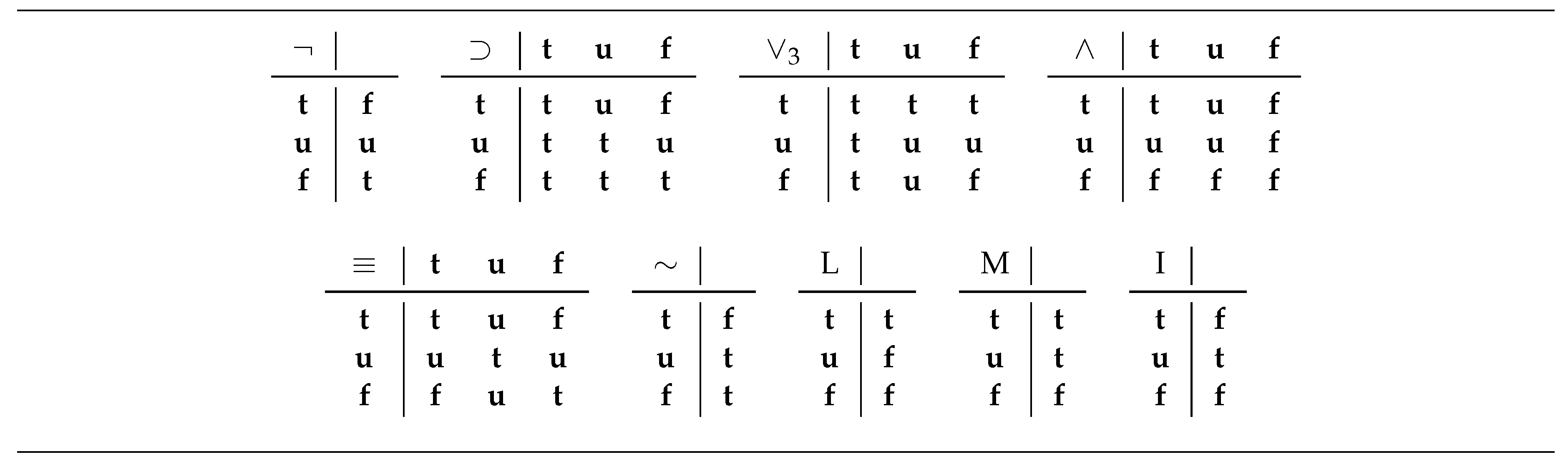
2.1.2. Łukasiewicz’s Three-Valued Logic

We now turn to the three-valued logic of Łukasiewicz [11] for the propositional case, henceforth denoted by ${\mathsf{Ł}}_{\mathbf{3}}$. Our presentation follows the one given by Radzikowska [9].

The alphabet of ${\mathsf{Ł}}_{\mathbf{3}}$ consists of the alphabet of $\mathbf{PL}$ along with the additional truth constant ⊔ (“undetermined”). Again, we assume $\mathcal{P}$ as a countable set of propositional constants. The class of formulas of ${\mathsf{Ł}}_{\mathbf{3}}$ is built similarly to the formulas of $\mathbf{PL}$, except that ⊔ is counted as an additional atomic formula.

A difference to the syntax of the logic $\mathbf{PL}$ concerns the defined connectives; while conjunction, $\wedge$, and material equivalence, $\equiv$, are defined as in propositional logic, disjunction in ${\mathsf{Ł}}_{\mathbf{3}}$ is defined differently:

$$\left(A{\vee }_{3}B\right):=((A\supset B)\supset B).$$

Furthermore, there are also additional unary defined operators, viz.

• the connective “$\sim$” (“weak negation”), given by

  $$\begin{array}{cc}\hfill \sim A:=& (A\supset \neg A);\hfill \end{array}$$
• the unary operators “$\mathrm{L}$” (“certainty operator”) and “$\mathrm{M}$” (“possibility operator”), defined by

  $$\mathrm{L}A:=\neg (A\supset \neg A)\mathrm{and}\mathrm{M}A:=(\neg A\supset A),$$

  which, according to Łukasiewicz [11], were first formalised in 1921 by Tarski; and
• the operator “$\mathrm{I}$”, given by

  $$\mathrm{I}A:=(\mathrm{M}A\wedge \neg \mathrm{L}A).$$

Intuitively, $\mathrm{L}A$ expresses that A is certain, whilst $\mathrm{M}A$ means that A is possible. These operators will be used subsequently to distinguish between certain knowledge and defeasible conclusions. Furthermore, $\mathrm{I}A$ expresses that A is contingent or modally indifferent.

A (three-valued) interpretation is a mapping m assigning to each propositional constant from $\mathcal{P}$ an element from $\{\mathbf{t},\mathbf{f},\mathbf{u}\}$. Here, besides the truth values $\mathbf{t}$ and $\mathbf{f}$, the symbol $\mathbf{u}$ represents a truth value standing for “undetermined” or “indeterminacy”. As usual, $m\left(P\right)$ is the truth value of P under m, where now P is true under an interpretation m if $m\left(P\right)=\mathbf{t}$, false under m if $m\left(P\right)=\mathbf{f}$, and has undetermined truth value if $m\left(P\right)=\mathbf{u}$.

The truth value, ${\mathrm{V}}^m\left(A\right)$, of an arbitrary formula A under an interpretation m is given subject to the following conditions:

• If $A=\mathsf{\top }$, then ${\mathrm{V}}^m\left(A\right)=\mathbf{t}$.
• If $A=\bigsqcup$, then ${\mathrm{V}}^m\left(A\right)=\mathbf{u}$.
• If $A=\mathsf{\perp }$, then ${\mathrm{V}}^m\left(A\right)=\mathbf{f}$.
• If A is an atomic formula, then ${\mathrm{V}}^m\left(A\right)=m\left(A\right)$.
• If $A=\neg B$, for some formula B, or $A=(C\supset D)$, for some formulas C and D, then ${\mathrm{V}}^m\left(A\right)$ is determined according to the truth tables given in Figure 1 (there, the corresponding truth conditions for the defined connectives are also given).

If ${\mathrm{V}}^m\left(A\right)=\mathbf{t}$, then A is true under m, if ${\mathrm{V}}^m\left(A\right)=\mathbf{u}$, then A is undetermined under m, and if ${\mathrm{V}}^m\left(A\right)=\mathbf{f}$, then A is false under m. If A is true under m, then m is a model of A. If A is true in every interpretation, then A is valid (in ${\mathsf{Ł}}_{\mathbf{3}}$), written ${\models }_{3}A$.

Clearly, the classically valid principle of tertium non datur, i.e., the law of excluded middle, $A\vee \neg A$, as well as the corresponding law of non-contradiction, $\neg (A\wedge \neg A)$, are not valid in ${\mathsf{Ł}}_{\mathbf{3}}$. However, their three-valued pendants, viz., the principle of quartum non datur, i.e., the law of excluded fourth, $A\vee \mathrm{I}A\vee \neg A$, and the corresponding extended non-contradiction principle, $\neg (A\wedge \neg \mathrm{I}A\wedge \neg A)$, are valid in ${\mathsf{Ł}}_{\mathbf{3}}$.

In classical logic, two formulas are logically equivalent if and only if, they have the same models, where logical equivalence between formulas A and B is defined by the condition that ${\models }_2(A\equiv B)$ holds. However, such a relation between logical equivalence and equality of models does not hold in general in the three-valued logic case. Indeed, following Radzikowska [9], let us define that two formulas A and B are strongly equivalent, symbolically $A{\iff }_{s}B$, iff ${\models }_3(A\equiv B)$. That is, A and B are strongly equivalent iff, for any three-valued interpretation m, ${\mathrm{V}}^m\left(A\right)={\mathrm{V}}^m\left(B\right)$. Furthermore, let us call A and B equivalent (in ${\mathsf{Ł}}_{\mathbf{3}}$), symbolically $A\iff B$, iff A and B have the same models. Clearly, strong equivalence implies equivalence, but in general not vice versa. For instance, P and $\mathrm{L}P$, for an atom P, are equivalent but not strongly equivalent. In addition, strong equivalence is an equivalence relation (i.e., reflexive, symmetric, and transitive) and enjoys a substitution principle, similar to the one of classical logic, i.e., if a formula $C_A$ contains a subformula A, and $C_B$ is the result of substituting at least one occurrence of A in $C_A$ by a formula B, then $A{\iff }_{s}B$ implies $C_A{\iff }_s{C}_B$.

Let us also note some strong equivalences which hold in ${\mathsf{Ł}}_{\mathbf{3}}$:

• $(A\supset B){\iff }_s(\mathrm{M}\neg A{\vee }_{3}B)\wedge (\mathrm{M}B{\vee }_3\neg A)$.
• $O(A\circ B){\iff }_s(OA\circ OB)$, for $O\in \{\mathrm{L},\mathrm{M}\}$ and $\circ \in \{\wedge ,\vee \}$.
• $O{O}^{\prime }A{\iff }_s{O}^{\prime }A$, for $O,O^{\prime }\in \{\mathrm{L},\mathrm{M}\}$.
• $\sim A{\iff }_s\mathrm{M}\neg A$.
• $\neg \mathrm{L}A{\iff }_s\mathrm{M}\neg A$.
• $\neg \mathrm{M}A{\iff }_s\mathrm{L}\neg A$.
• $((A\wedge B){\vee }_{3}C{\iff }_s\left(A{\vee }_{3}C\right)\wedge \left(B{\vee }_{3}C\right)$.
• $(\left(A{\vee }_{3}B\right)\wedge C{\iff }_s(A\wedge C){\vee }_3(B\wedge C)$.

The notion of a theory in ${\mathsf{Ł}}_{\mathbf{3}}$ is defined as in $\mathbf{PL}$, i.e., a theory is a set of formulas. Likewise, the notion of a model or of a countermodel of a theory, and of a theory being satisfiable, falsifiable (or refutable), or unsatisfiable are defined in ${\mathsf{Ł}}_{\mathbf{3}}$ mutatis mutandis as in $\mathbf{PL}$. A theory T is said to entail a formula A (in ${\mathsf{Ł}}_{\mathbf{3}}$), or A is a valid consequence of T (in ${\mathsf{Ł}}_{\mathbf{3}}$), symbolically $T{\models }_{3}A$, iff every model (in ${\mathsf{Ł}}_{\mathbf{3}}$) of T is also a model (in ${\mathsf{Ł}}_{\mathbf{3}}$) of A.

Sound and complete Hilbert-style axiomatisations of the logic ${\mathsf{Ł}}_{\mathbf{3}}$ can be readily found in the literature [47,48]; the first one was introduced by Wajsberg in 1931 [49]. We write $T{⊢}_{3}A$ if A has a derivation (in some fixed Hilbert-style calculus) from T in ${\mathsf{Ł}}_{\mathbf{3}}$. As well, the deductive closure operator of ${\mathsf{Ł}}_{\mathbf{3}}$ is given by

$${\mathrm{Th}}_3\left(T\right):=\{A\mid T{⊢}_{3}A\},$$

where T is a theory. The notions of a theory being deductively closed and of being consistent, as well as of a formula being consistent with a theory, are defined similarly as in $\mathbf{PL}$. Moreover, the properties of inflationaryness, idempotency, and monotonicity hold for ${\mathrm{Th}}_3(·)$ like for ${\mathrm{Th}}_2(·)$, and consistency of a theory T in ${\mathsf{Ł}}_{\mathbf{3}}$ is equivalent to the satisfiability of T in ${\mathsf{Ł}}_{\mathbf{3}}$.

While in $\mathbf{PL}$ we have the well-known properties that (i) $T{⊢}_{2}A$ iff $T\cup \{\neg A\}$ is inconsistent and (ii) $T,A{⊢}_{2}B$ iff $T{⊢}_2(A\supset B)$ (the “only if” part of the latter is generally referred to as the deduction theorem), for a theory T and formulas A and B, in ${\mathsf{Ł}}_{\mathbf{3}}$ sight variations thereof hold:

Proposition 1.

Let T be a theory, and A and B formulas.

1. 

$T{⊢}_{3}A$ iff $T\cup \{\mathrm{M}\neg A\}$ is inconsistent (in ${\mathsf{Ł}}_{\mathbf{3}}$).

2. 

$T,A{⊢}_{3}B$ iff $T{⊢}_3(\mathrm{L}A\supset B)$.

Note that, as a consequence, the consistency of a formula A with a theory T implies the consistency of the theory $T\cup \left\{\mathrm{M}A\right\}$, but it does not necessarily imply the consistency of $T\cup \left\{A\right\}$. For instance, $\neg P$ is consistent with $\left\{\mathrm{M}P\right\}$, for an atomic formula P, so $\{\mathrm{M}P,\mathrm{M}\neg P\}$ is consistent, but $\{\mathrm{M}P,\neg P\}$ is not.

Furthermore, although in ${\mathsf{Ł}}_{\mathbf{3}}$ it always holds that $T{⊢}_{3}A\supset B$ implies $T,A{⊢}_{3}B$, it is the converse direction (i.e., the classical version of the deduction theorem) that fails in general.

2.2. Two Variants of Default Logic

We continue with the basic elements of three-valued default logic, due to Radzikowska [9], and of disjunctive default logic, introduced by Gelfond, Lifschitz, Przymusinska, and Truszczyński [10]. Note that we deal here with propositional versions of the formalisms as our subsequent calculi are defined for the propositional case only, similar to the undertaking of Bonatti [7,37] and of Bonatti and Olivetti [8].

2.2.1. Three-Valued Default Logic

Radzikowska’s three-valued default logic [9], which in what follows we will denote by ${\mathbf{DL}}_{\mathbf{3}}$, differs from Reiter’s standard default logic [1] (henceforth referred to as $\mathbf{DL}$) in two aspects; not only is in ${\mathbf{DL}}_{\mathbf{3}}$ the deductive machinery of classical logic replaced with ${\mathsf{Ł}}_{\mathbf{3}}$, but there is also a modified consistency check for default rules employed in which the consequent of a default is taken into account as well. The latter feature is somewhat reminiscent to the consistency checks used in justified default logic [12] and in constrained default logic [13,14], where a default may only be applied if it does not lead to a contradiction a posteriori.

Formally, a default rule, or simply a default, d, is an expression of the form

$${\displaystyle \frac{A:B_1,\dots ,B_n}{C},}$$

where A is the prerequisite, $B_1,\dots ,B_n$ are the justifications, and C is the consequent of d. The intuitive meaning of such a default is:

if A is believed, and $B_1,\dots ,B_n$ and $\mathrm{L}C$ are consistent with what is believed, then $\mathrm{M}C$ is asserted.

Note that under this reading, by applying a default of the above form, it is assumed that C cannot be false, but it is not assumed that C is true in all situations. It is only assumed that C must be true in at least one such situation. This reflects the intuition that accepting a default conclusion, we are prepared to rule out all situations where it is false, but we can imagine at least one such situation in which it is true. As a consequence, we cannot conclude both $\mathrm{M}C$ and $\mathrm{M}\neg C$ simultaneously.

In what follows, formulas of the form $\mathrm{M}C$ obtained by applying defaults will be referred to as default assumptions. For simplicity, defaults will also be written in the form $(A:B_1,\dots ,B_n/C)$.

A default theory, T, is a pair $\langle W,D\rangle$, where W is a set of formulas (i.e., a theory in ${\mathsf{Ł}}_{\mathbf{3}}$), called the premisses of T, and D is a set of defaults. An extension of a default theory $T=\langle W,D\rangle$ in the three-valued default logic ${\mathbf{DL}}_{\mathbf{3}}$ is defined thus: For a set S of formulas, let ${\Gamma }_T\left(S\right)$ be the smallest set K of formulas obeying the following conditions:

• $K={\mathrm{Th}}_3\left(K\right)$.
• $W\subseteq K$.
• If $(A:B_1,\dots ,B_n/C)\in D$, $A\in K$, $\neg B_1\notin S,\dots ,\neg B_n\notin S$, and $\neg \mathrm{L}C\notin S$, then $\mathrm{M}C\in K$.

Then, E is an extension of T iff ${\Gamma }_T\left(E\right)=E$.

Note that the criterion of the applicability of a default in ${\mathbf{DL}}_{\mathbf{3}}$ makes the two defaults:

$$d=\frac{A:B_1,\dots ,B_n}{C}\mathrm{and}{d}^{\prime }=\frac{A:\mathrm{M}{B}_1,\dots ,\mathrm{M}{B}_n}{C}$$

equivalent in the sense that the application of d implies the application of $d^{\prime }$ and vice versa. Thus, in a default theory $T=\langle W,D\rangle$, we can replace every $d\in D$ with its corresponding version $d^{\prime }$ without changing extensions.

Note further that, for obtaining extensions in the sense of Reiter [1], in the above definition, instead of ${\mathrm{Th}}_3(·)$ we use ${\mathrm{Th}}_2(·)$, and the condition 3 is replaced by:

3’.

If $(A:B_1,\dots ,B_n/C)\in D$, $A\in K$, and $\neg B_1\notin S,\dots ,\neg B_n\notin S$, then $C\in K$.

There are two basic reasoning tasks in the context of default logic, viz., brave reasoning and skeptical reasoning. The former task is the problem of checking whether a formula A belongs to at least one extension of a given default theory T, whilst the latter task examines whether A belongs to all extensions of T. Our aim is to give a sequent-type axiomatisation of brave default reasoning, following the approach of Bonatti [7] for standard default logic.

To conclude our review of three-valued default logic, we give two examples, as discussed by Radzikowska [9], showing the representational advantages of ${\mathbf{DL}}_{\mathbf{3}}$.

Example 1

([50]).Consider the default theory $T=\langle W,D\rangle$, where

$$W=\{\mathit{Summer},\neg \mathit{Sun}\_\mathit{Shining}\}andD=\left\{\frac{\mathit{Summer}:\neg \mathit{Rain}}{\mathit{Sun}\_\mathit{Shining}}\right\}.$$

The only default of this theory is inapplicable since $W{⊢}_3\neg \mathrm{L}\mathit{Sun}\_\mathit{Shining}$ holds. Hence, T has a single extension, viz. $E={\mathrm{Th}}_3\left(W\right)$. Note that T has no extension in Reiter’s default logic due to the weaker consistency check which results in a vicious circle where the application of the default violates its justification for applying it.

Example 2

([51]).Consider the default rules

$$d_1=\frac{P:Q}{Q}and{d}_2=\frac{Q:R}{R},$$

where P, Q, and R stand for the following propositions:

• P: “Tony recites passages from Shakespeare”;
• Q: “Tony can read and write”;
• R: “Tony is over seven years old”.

Obviously, common sense suggests that, given P, there are perfect reasons to apply both defaults to infer that Tony is over seven years old. Suppose now that we add the default rule

$$d_3=\frac{S:Q}{Q},$$

where S stands for “Tony is a child prodigy”. Given S, it is reasonable to infer that Tony can read and write, but the inference of R that Tony is over seven years old seems to be unjustified.

In standard default logic $\mathbf{DL}$, a common way of suppressing R in the latter scenario would be to employ a default rule with exceptions of the form

$$d_2^{\prime }=\frac{Q:R\wedge \neg S}{R}.$$

However, this remedy is somewhat unsatisfactory as it requires that every default may possess a potentially large number of conceivable exceptions which, each time a new default is added, the previous ones must be revised, which is arguably ad hoc. In ${\mathbf{DL}}_{\mathbf{3}}$, on the other hand, this can easily be accommodated by using the defaults

$$\frac{P:\mathrm{L}Q}{\mathrm{L}Q}and\frac{Q:\mathrm{L}R}{\mathrm{L}R}$$

instead of $d_1$ and $d_2$, as well as

$$\frac{\mathrm{M}S:Q}{Q}$$

instead of $d_3$.

Actually, the last example illustrates the difference between causal rules (“expectation-evoking rules”) and evidential rules (“explanation-evoking rules”) [51]. An example of the first kind of rules is “fire usually causes smoke” whilst “smoke usually suggests fire” is an instance of the second kind. As argued by Pearl [51], an evidential rule should not be applied if its prerequisite is derived by applying at least one causal rule. In ${\mathbf{DL}}_{\mathbf{3}}$, this can be taken into account by formalising causal default rules in the form of $(\mathrm{M}A:B/B)$, $(\mathrm{L}A:B/B)$, or $(A:B/B)$, whilst evidential rules are formalised by $(\mathrm{L}A:\mathrm{L}B/\mathrm{L}B)$ or, equivalently, by $(A:\mathrm{L}B/\mathrm{L}B)$.

2.2.2. Disjunctive Default Logic

We now turn to the basics of disjunctive default logic [10], henceforth referred to as ${\mathbf{DL}}_{\mathbf{D}}$.

The main motivation for introducing disjunctive default logics was to address a difficulty encountered when using defaults in the presence of disjunctive information, a problem which was first observed by David Poole [52]. More specifically, the difficulty lies in the difference between a default theory having two extensions, one containing a formula A and the other a formula B, and a theory with a single extension, containing the disjunction $A\vee B$. This problem was also noted by Lin and Shoham [53], who gave an example of a theory in a modal-logic language, containing disjunctive information, and observed that no default theory exists which corresponds to this theory.

Another nice feature of disjunctive default logic is that it provides a one-to-one correspondence between answer-sets of disjunctive logic programs [4] and extensions of a corresponding disjunctive default theory. Such a correspondence does likewise not directly hold for standard default logic—and again the key problem lies in the presence of disjunctive information. More specifically, viewing $P\vee Q$ as a rule in a logic program under the answer-set semantics, the default naturally corresponding to this rule would be the default rule

$$d=\frac{\mathsf{\top }:}{P\vee Q}.$$

Now, while the program consisting of the single rule $P\vee Q$ has two answer sets, viz. $\left\{P\right\}$ and $\left\{Q\right\}$, the default theory $\langle \varnothing ,\left\{d\right\}\rangle$ has only one extension, ${\mathrm{Th}}_2\left(\{P\vee Q\}\right)$. As long as only programs without disjunctions are considered, such a natural translation of program rules into defaults gives rise to a one-to-one correspondence between answer sets of the given program and the extensions of its translation.

To formally introduce ${\mathbf{DL}}_{\mathbf{D}}$, by a disjunctive default rule, or simply a disjunctive default, d, we understand an expression of the form

$${\displaystyle \frac{A:B_1,\dots ,B_n}{C_1|\cdots |C_m},}$$

where A, $B_1$, …,$B_n$, and $C_1$, …,$C_m$ are formulas from $\mathbf{PL}$. Similar to ${\mathbf{DL}}_{\mathbf{3}}$, we call A the prerequisite, $B_1,\dots ,B_n$ the justifications, and $C_1,\dots ,C_n$ the consequents of d. Furthermore, following Baumgartner and Gottlob [54], we refer to the symbol “|” as effective disjunction.

The intuitive meaning of such a default is:

if A is believed and $B_1,\dots ,B_n$ are consistent with what is believed, then one of $C_1,\dots ,C_m$ is asserted.

Similar to conventions in standard default logic, if the prerequisite of a default d is ⊤, then we will omit it from d. If, additionally, d has no justifications, then d is simply written as

$$C_1|\cdots |C_m,$$

where $C_1,\dots ,C_m$ are the consequents of d. For convenience, disjunctive defaults will also be written in the form $(A:B_1,\dots ,B_n/C_1|\cdots \left|C_m\right)$.

A disjunctive default theory, T, is a pair $\langle W,D\rangle$, where W is a set of formulas of $\mathbf{PL}$ (again referred to as the premisses of T) and D is a set of disjunctive defaults.

For defining extensions of disjunctive default theories, we need some further notation: Let us call a set S of formulas closed under propositional consequence if, whenever $S{⊢}_{2}A$, then $A\in S$. Clearly, the deductive closure of a set S, ${\mathrm{Th}}_2\left(S\right)$, is the smallest set of formulas closed under propositional consequence containing S. Moreover, for a family F of sets, let $min\left(F\right)$ denote the minimal elements of F, where minimality is defined with respect to set inclusion, i.e.,

$$min\left(F\right)=\{X\mid X\in F\hspace{0.17em}\text{and\hspace{0.17em}there\hspace{0.17em}is\hspace{0.17em}no}\hspace{0.17em}Z\in F\hspace{0.17em}\text{such\hspace{0.17em}that}\hspace{0.17em}Z\subset X\}.$$

Consider now a disjunctive default theory $T=\langle W,D\rangle$. Given a set S of formulas of $\mathbf{PL}$, let ${\mathit{Cl}}_T\left(S\right)$ be the collection of all sets K satisfying the following conditions:

• $K={\mathrm{Th}}_2\left(K\right)$.
• $W\subseteq K$.
• If $(A:B_1,\dots ,B_n/C_1|\cdots \left|C_m\right)\in D$, $A\in K$ and $\{\neg B_1,\dots ,\neg B_n\}\cap S=\varnothing$, then $C_i\in K$, for some $i\in \{1,\dots ,m\}$.

Moreover, let ${\Delta }_T\left(S\right)=min\left({\mathit{Cl}}_T\left(S\right)\right)$, i.e., ${\Delta }_T\left(S\right)$ consists of all minimal sets obeying conditions 1–3. Then, a set E of formulas of $\mathbf{PL}$ is an extension of T if $E\in {\Delta }_T\left(E\right)$.

The notion of a brave and a skeptical consequence given a disjunctive default theory is defined as before mutatis mutandis.

Let us now discuss some examples showing the differences between disjunctive default logic and standard default logic, following Gelfond, Lifschitz, Przymusinska, and Truszczyński [10].

Example 3

([1]).Consider the default theory $T=\langle W,D\rangle$, for

$$W=\{P\vee Q\}andD=\left\{\frac{P:R}{R},\frac{Q:S}{S}\right\},$$

where P, Q, R, and S are atomic formulas. Intuitively, given the disjunctive information $P\vee Q$, we would expect to derive $R\vee S$, because, in case P holds, we could apply the first default, and in case Q holds, we could accordingly apply the second default. However, in $\mathbf{DL}$, neither of the two defaults is applicable and the single extension of T is ${\mathrm{Th}}_2\left(W\right)$.

Now, in disjunctive default logic, we can represent the information expressed by T in terms of a disjunctive default theory $T^{\prime }$ containing the three defaults

$$P|Q,\frac{P:R}{R},and\frac{Q:S}{S}.$$

In contrast to the situation in $\mathbf{DL}$, $T^{\prime }$ possesses two extensions in ${\mathbf{DL}}_{\mathbf{D}}$, viz. ${\mathrm{Th}}_2\left(\{P,R\}\right)$ and ${\mathrm{Th}}_2\left(\{Q,S\}\right)$, and $R\vee S$ is contained in both, which is in accordance to our expectations.

We next discuss the example by Poole [52].

Example 4.

Let us assume the following commonsense information: By default, a person’s left arm is usable, the exception being when it is broken, and similarly for the right arm.

In standard default logic, we can express this by the following two defaults:

$$d_1:=\frac{:U_l\wedge \neg B_l}{U_l}and{d}_2:=\frac{:U_r\wedge \neg B_r}{U_r},$$

where “$U_l$” and “$U_r$” stand for that the left arm is usable and that the right arm is usable, respectively, and, similarly, “$B_l$” and “$B_r$” mean that the left arm or the right arm is broken.

If there is no further information about one’s hands, then one can conclude that both hands are usable. Indeed, the default theory $T=\langle \varnothing ,\{d_1,d_2\}\rangle$ has a single extension in $\mathbf{DL}$, containing both $U_l$ and $U_r$.

However, if it is now known that the left arm is broken, i.e., $B_l$ is asserted, then the application of $d_1$ is blocked and the extended default theory

$$T^{\prime }=\langle \left\{B_l\right\},\{d_1,d_2\}\rangle$$

has again one extension, containing $U_r$.

But let us assume now that we only know that one arm is broken, but we do not remember exactly which one. So, what we can assert now is the formula

$$B_l\vee B_r.$$

Considering now the extensions of the default theory

$$T^{″}=\langle \{B_l\vee B_r\},\{d_1,d_2\}\rangle ,$$

this default theory has still one extension, but unfortunately it contains both $U_l\vee U_r$, which is contrary to our intuition.

Using ${\mathbf{DL}}_{\mathbf{D}}$, on the other hand, we can represent the information of $T^{″}$ by a disjunctive default theory containing

$$B_l|B_r$$

together with the two defaults $d_1$ and $d_2$. The resulting theory has two extensions, viz.

$${\mathrm{Th}}_2\left(\{B_l,U_r\}\right)and{\mathrm{Th}}_2\left(\{B_r,U_l\}\right),$$

both containing

$$U_l\vee U_r,$$

which corresponds with our intuition.

Note that the difference between a formula $A\vee B$ and a disjunctive default $A|B$ amounts to the difference between the assertions “A or B is known” and “A is known or B is known”.

3. A Sequent Calculus for Three-Valued Default Logic

We now introduce our sequent calculus ${\mathsf{B}}_3$ for brave reasoning in ${\mathbf{DL}}_{\mathbf{3}}$. Following the general design of the approach of Bonatti [7,55], ${\mathsf{B}}_3$ involves three kinds of sequents, viz. assertional sequents for axiomatising validity in ${\mathsf{Ł}}_{\mathbf{3}}$, anti-sequents for axiomatising non-tautologies of ${\mathsf{Ł}}_{\mathbf{3}}$, and special default sequents representing brave reasoning in $\mathbf{DL}$.

We start with laying down the postulates of ${\mathsf{B}}_3$ and then, in Section 3.2, we show soundness and completeness.

3.1. Postulates of the Calculus

As far as sequent-type calculi for three-valued logics are concerned,—or, more generally, many-valued logics—different techniques have been discussed in the literature [21,24,26,56,57,58]. Here, we use an approach due to Rousseau [25], which is a natural generalisation for many-valued logics of the classical two-sided sequent formulation as pioneered by Gentzen [23]. In Rousseau’s approach, a sequent for a three-valued logic is a triple of sets of formulas where each component of the sequent represents one of the three truth values.

3.1.1. A Sequent Calculus for ${\mathsf{Ł}}_{\mathbf{3}}$

Formally, we introduce sequents for ${\mathsf{Ł}}_{\mathbf{3}}$ as follows:

Definition 1.

A (three-valued) sequent is a triple of the form ${\Gamma }_1\mid {\Gamma }_2\mid {\Gamma }_3$, where each ${\Gamma }_i$, for $i\in \{1,2,3\}$, is a finite set of formulas, called a component of the sequent.

For a (three-valued) interpretation m, a sequent ${\Gamma }_1\mid {\Gamma }_2\mid {\Gamma }_3$ is true under m if, for at least one $i\in \{1,2,3\}$, ${\Gamma }_i$ contains some formula A such that ${\mathrm{V}}^m\left(A\right)={\mathsf{v}}_i$, where ${\mathsf{v}}_1=\mathbf{f}$, ${\mathsf{v}}_2=\mathbf{u}$, and ${\mathsf{v}}_3=\mathbf{t}$. Furthermore, a sequent is valid if it is true under each interpretation.

Note that a standard classical sequent $\Gamma ⊢\Delta$ in the sense of Gentzen [23] corresponds to a pair $\Gamma \mid \Delta$ under the usual two-valued semantics of $\mathbf{PL}$.

As customary for sequents, we write sequent components comprised of a singleton set $\left\{A\right\}$ simply as “A”, and likewise we write $\Gamma \cup \left\{A\right\}$ as “$\Gamma ,A$”.

For obtaining the postulates of a many-valued logic in Rousseau’s approach, the conditions of the logical connectives of a given logic are encoded in two-valued logic by means of a so-called partial normal form [47] and expressed by suitable inference rules.

The calculus we employ for ${\mathsf{Ł}}_{\mathbf{3}}$, which we denote by $\mathsf{S}{\mathsf{Ł}}_3$, is taken from Zach [26], which is obtained from a systematic construction of sequent-style calculi for many-valued logics and by applying some optimisations of the corresponding partial normal forms.

Definition 2.

The postulates of $\mathsf{S}{\mathsf{Ł}}_3$ are as follows:

• axioms of $\mathsf{S}{\mathsf{Ł}}_3$ are sequents of the form

  -

  $\mathsf{\perp }\mid \varnothing \mid \varnothing$,

  -

  $\varnothing \mid \bigsqcup \mid \varnothing$,

  -

  $\varnothing \mid \varnothing \mid \mathsf{\top }$, and

  -

  $A\mid A\mid A$, where A is a formula;

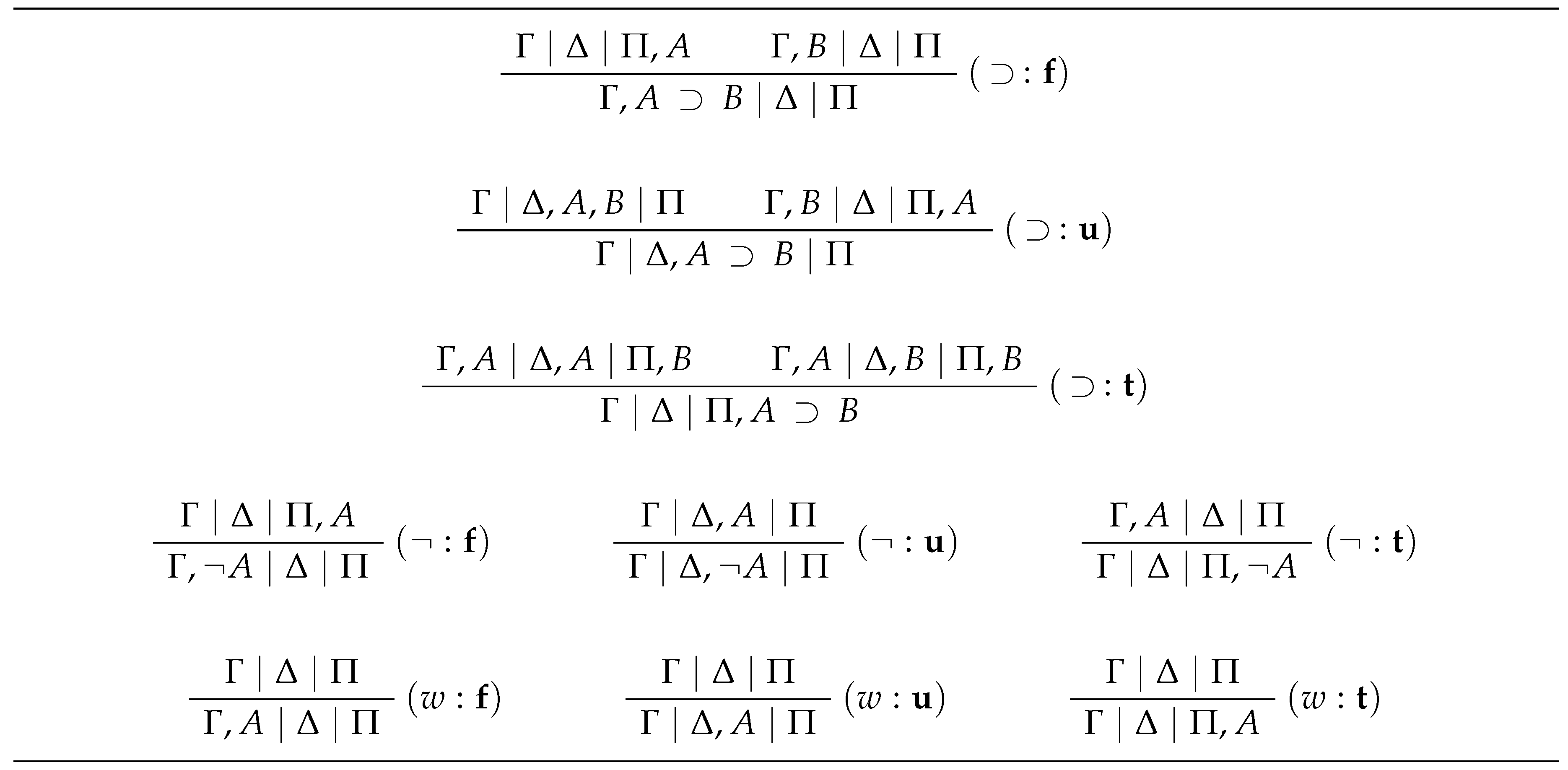
  and
• the inference rules of $\mathsf{S}{\mathsf{Ł}}_3$ are comprised of the rules depicted in Figure 2.

Note that from the inference rules of $\mathsf{S}{\mathsf{Ł}}_3$, we can easily obtain derived rules for the defined connectives of ${\mathsf{Ł}}_{\mathbf{3}}$. Furthermore, the last three rules in Figure 2 are also referred to as weakening rules.

Soundness and completeness of $\mathsf{S}{\mathsf{Ł}}_3$ follows directly from the method AS described by Zach [26]:

Proposition 2.

A sequent $\Gamma \mid \Delta \mid \Pi$ is valid iff it is provable in$\mathsf{S}{\mathsf{Ł}}_3$.

Note that sequents in the style of Rousseau are truth functional rather than formalising entailment directly, but, by a general result for many-valued logics as shown by Zach [26], the latter can be expressed simply as follows:

Proposition 3.

For a theory T and a formula A, $T{⊢}_{3}A$ iff the sequent $T\mid T\mid A$ is provable in$\mathsf{S}{\mathsf{Ł}}_3$.

3.1.2. An Anti-Sequent Calculus for ${\mathsf{Ł}}_{\mathbf{3}}$

As for axiomatising non-theorems of ${\mathsf{Ł}}_{\mathbf{3}}$, a systematic construction of rejection calculi for many-valued logics has been developed by Bogojeski and Tompits [27], based on adapting the approach of Zach [26]. The refutation calculus we describe now for axiomatising invalid sequents in ${\mathsf{Ł}}_{\mathbf{3}}$, denoted by $\mathsf{R}{\mathsf{Ł}}_3$, is obtained from the method of Bogojeski and Tompits [27].

Definition 3.

A (three-valued) anti-sequent is a triple of form ${\Gamma }_1\nmid {\Gamma }_2\nmid {\Gamma }_3$, where each ${\Gamma }_i$, for $i\in \{1,2,3\}$, is a finite set of formulas, called a component of the anti-sequent.

For a (three-valued) interpretation m, an anti-sequent ${\Gamma }_1\nmid {\Gamma }_2\nmid {\Gamma }_3$ is refuted by m, or m refutes ${\Gamma }_1\nmid {\Gamma }_2\nmid {\Gamma }_3$, if, for every $i\in \{1,2,3\}$ and every formula $A\in {\Gamma }_i$, ${\mathrm{V}}^m\left(A\right)\ne {\mathsf{v}}_i$, where ${\mathsf{v}}_i$ is defined as in Definition 1. An anti-sequent ${\Gamma }_1\nmid {\Gamma }_2\nmid {\Gamma }_3$ is refutable if there is at least one interpretation that refutes ${\Gamma }_1\nmid {\Gamma }_2\nmid {\Gamma }_3$.

Clearly, an anti-sequent ${\Gamma }_1\nmid {\Gamma }_2\nmid {\Gamma }_3$ is refutable iff the corresponding sequent ${\Gamma }_1\mid {\Gamma }_2\mid {\Gamma }_3$ is not valid.

Definition 4.

The postulates of $\mathsf{R}{\mathsf{Ł}}_3$ are as follows:

• the axioms of $\mathsf{R}{\mathsf{Ł}}_3$ are anti-sequents of the form ${\Gamma }_1\nmid {\Gamma }_2\nmid {\Gamma }_3$, where each ${\Gamma }_i$ ($i\in \{1,2,3\}$) is a set of atomic formulas such that ${\Gamma }_1\cap {\Gamma }_2\cap {\Gamma }_3=\varnothing$, $\mathsf{\top }\notin {\Gamma }_1$, $\bigsqcup \notin {\Gamma }_2$, and $\mathsf{\perp }\notin {\Gamma }_3$; and
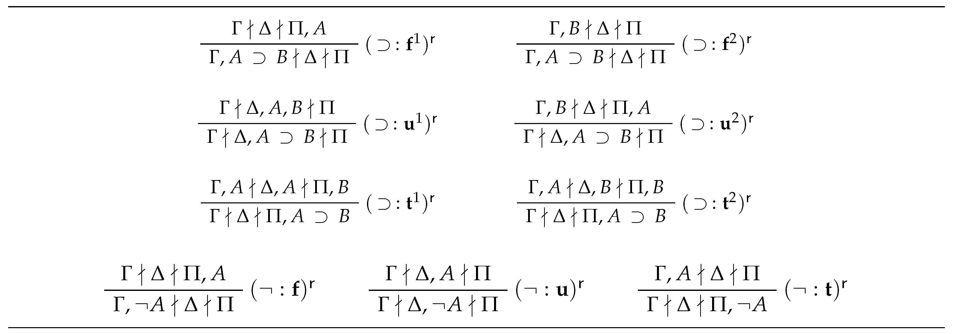
• the inference rules of $\mathsf{R}{\mathsf{Ł}}_3$ are those given in Figure 3.

Note that, in contrast to $\mathsf{S}{\mathsf{Ł}}_3$, the inference rules of $\mathsf{R}{\mathsf{Ł}}_3$ have only single premisses. Indeed, this is a general pattern in sequent-style rejection calculi: If an inference rule for standard (assertional) sequents for a connective has n premisses, then there are usually n corresponding unary inference rules in the associated rejection calculus. Intuitively, what is an exhaustive search in a standard sequent calculus becomes nondeterminism in a rejection calculus.

Again, soundness and completeness of $\mathsf{R}{\mathsf{Ł}}_3$ follow from the systematic construction as described by Bogojeski and Tompits [27]. Likewise, non-entailment in ${\mathsf{Ł}}_{\mathbf{3}}$ is expressed similarly as for $\mathsf{S}{\mathsf{Ł}}_3$.

Proposition 4.

An anti-sequent $\Gamma \nmid \Delta \nmid \Pi$ is refutable iff it is provable in$\mathsf{R}{\mathsf{Ł}}_3$.

Proposition 5.

For a theory T and a formula A, $T{⊬}_{3}A$ iff $T\nmid T\nmid A$ is provable in$\mathsf{R}{\mathsf{Ł}}_3$.

3.1.3. The Default-Sequent Calculus ${\mathsf{B}}_3$

We are now in a position to specify our calculus ${\mathsf{B}}_3$ for brave reasoning in ${\mathbf{DL}}_{\mathbf{3}}$.

Definition 5.

A (brave) default sequent is an ordered quadruple of the form $\Gamma ;\Delta \Rightarrow \Sigma ;\Theta$, where Γ, Σ, and Θ are finite sets of formulas and Δ is a finite set of defaults.

A default sequent $\Gamma ;\Delta \Rightarrow \Sigma ;\Theta$ is true if there is an extension E of the default theory $\langle \Gamma ,\Delta \rangle$ such that $\Sigma \subseteq E$ and $\Theta \cap E=\varnothing$; E is called a witness of $\Gamma ;\Delta \Rightarrow \Sigma ;\Theta$.

The default sequent calculus ${\mathsf{B}}_3$ consists of three-valued sequents, anti-sequents, and default sequents. It incorporates the systems $\mathsf{S}{\mathsf{Ł}}_3$ for three-valued sequents and $\mathsf{R}{\mathsf{Ł}}_3$ for anti-sequents, as well as additional axioms and inference rules for default sequents, described as follows:

Definition 6.

The postulates of ${\mathsf{B}}_3$ comprise the following items:

• all axioms and inference rules of $\mathsf{S}{\mathsf{Ł}}_3$ and $\mathsf{R}{\mathsf{Ł}}_3$;
• axioms of the form $\Gamma ;\varnothing \Rightarrow \varnothing ;\varnothing$, where Γ is a finite set of formulas of${\mathsf{Ł}}_{\mathbf{3}}$; and
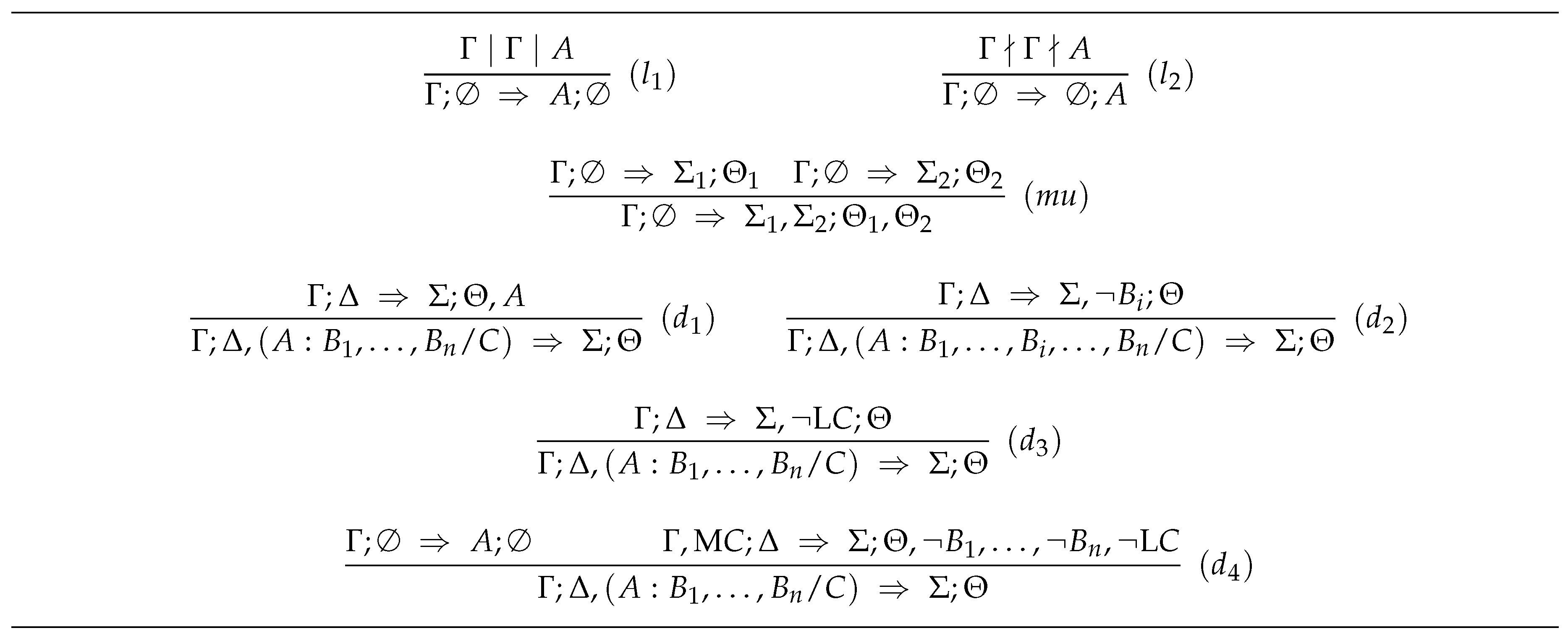
• the inference rules depicted in Figure 4.

The informal meaning of the inference rules for the default sequents is the following:

(i)

rules $\left(l_1\right)$ and $\left(l_2\right)$ combine three-valued sequents and anti-sequents with default sequents, respectively;

(ii)

rule $\left(\mathit{mu}\right)$ is the rule of “monotonic union”—it allows the joining of information in case that no default is present; and

(iii)

rules $\left(d_1\right)$–$\left(d_4\right)$ are the default introduction rules, where rules $\left(d_1\right)$, $\left(d_2\right)$, and $\left(d_3\right)$ take care of introducing non-active defaults, whilst rule $\left(d_4\right)$ allows to introduce an active default.

Let us give an example to illustrate the functioning of the calculus.

Example 5.

Consider the default theory $T=\langle W,D\rangle$ from Example 1, where

$$W=\{\mathit{Summer},\neg \mathit{Sun}\_\mathit{Shining}\}andD=\left\{\frac{\mathit{Summer}:\neg \mathit{Rain}}{\mathit{Sun}\_\mathit{Shining}}\right\}.$$

As we saw, the single default of this theory is inapplicable since $W{⊢}_3\neg \mathrm{L}\mathit{Sun}\_\mathit{Shining}$ and $E={\mathrm{Th}}_3\left(W\right)$ is therefore the only extension of T. Consequently, $\mathit{Sun}\_\mathit{Shining}\notin E$ also holds. Hence, the default sequent

$$\mathit{Summer},\neg \mathit{Sun}\_\mathit{Shining};(\mathit{Summer}:\neg \mathit{Rain}/\mathit{Sun}\_\mathit{Shining})\Rightarrow \neg \mathrm{L}\mathit{Sun}\_\mathit{Shining};\mathit{Sun}\_\mathit{Shining}$$

(1)

is true. We will give a proof of (1) in ${\mathsf{B}}_3$.

The proof of (1), depicted below and denoted by β, uses the proof α as subproof. For brevity, we will use “S“ for “$\mathit{Summer}$”, “R” for “$\mathit{Rain}$”, and “H” for $\mathit{Sun}\_\mathit{Shining}$”.

• Proof α:
• Proof β:

3.2. Adequacy of the Calculus

We now show soundness and completeness of ${\mathsf{B}}_3$. To this end, we need some auxiliary results first, dealing with alternative characterisations and properties of extensions.

3.2.1. Preparatory Characterisations: Residues and Extensions

We start with some properties of extensions concerning adding defaults to default theories which provide the groundwork on which our adequacy proofs are built. In doing so, we first introduce an alternative formulation of ${\mathbf{DL}}_{\mathbf{3}}$ extensions, adapting a proof-theoretical characterisation as described by Marek and Truszczyński [59] for standard default logic, and afterwards we provide results concerning so-called residues, which are inference rules resulting from defaults satisfying their consistency conditions. The latter endeavour generalises the approach of Bonatti [7] to the three-valued case.

Definition 7.

Let E be a set of formulas. A default $(A:B_1,\dots ,B_n/C)$ is ${\mathbf{DL}}_{\mathbf{3}}$-active in E iff $E{⊢}_{3}A$ and $\{\neg B_1,\dots ,\neg B_n,\neg \mathrm{L}C\}\cap E=\varnothing$.

Definition 8.

Let D be a set of defaults and E a set of formulas. The ${\mathbf{DL}}_{\mathbf{3}}$-reduct of D with respect to E, denoted by $D_E$, is the set consisting of the following inference rules:

$$\begin{array}{ccc}\hfill D_E& :=& \left.{\displaystyle \left\{{\displaystyle \frac{A}{\mathrm{M}C}}\right|\frac{A:B_1,\dots ,B_n}{C}\in D\hspace{0.17em}and\{\neg B_1,\dots ,\neg B_n,\neg \mathrm{L}C\}\cap E=\varnothing }\right\}.\hfill \end{array}$$

An inference rule $A/\mathrm{M}C$ is called ${\mathbf{DL}}_{\mathbf{3}}$-residue of a default $(A:B_1,\dots ,B_n/C)$.

Whenever it is clear from the context, we will allow ourselves to drop the prefix “${\mathbf{DL}}_{\mathbf{3}}$-” in “${\mathbf{DL}}_{\mathbf{3}}$-active”, “${\mathbf{DL}}_{\mathbf{3}}$-reduct”, and “${\mathbf{DL}}_{\mathbf{3}}$-residue” to ease notation.

For a set R of inference rules, let ${⊢}_3^R$ be the inference relation obtained from ${⊢}_3$ by augmenting the postulates of the Hilbert-type calculus for ${\mathsf{Ł}}_{\mathbf{3}}$ underlying the relation ${⊢}_3$ with the inference rules from R. Let the corresponding deductive closure operator for ${⊢}_3^R$ be given by

$${\mathrm{Th}}_3^R\left(W\right):=\{A\mid W{⊢}_3^{R}A\}.$$

Clearly, ${\mathrm{Th}}_3^{\varnothing }\left(W\right)={\mathrm{Th}}_3\left(W\right)$.

We then obtain the following characterisation of the operator ${\Gamma }_T$, mirroring the analogous property for standard default logic as discussed by Marek and Truszczyński [59]:

Theorem 1.

Let $T=\langle W,D\rangle$ be a three-valued default theory, E a set of formulas of${\mathsf{Ł}}_{\mathbf{3}}$, and $D_E$ the ${\mathbf{DL}}_{\mathbf{3}}$-reduct of D with respect to E. Then,

$${\Gamma }_T\left(E\right)={\mathrm{Th}}_3^{D_E}\left(W\right).$$

Proof. 

The result follows by a straightforward adaption of the proof of the analogous result for the case of standard default logic as given by Marek and Truszczyński [59].  □

By the definition of an extension, we thus obtain:

Corollary 1.

Let $T=\langle W,D\rangle$ be a three-valued default theory and E a set of formulas. Then,

$$E\hspace{0.17em}\mathit{is}\hspace{0.17em}\mathit{an}\hspace{0.17em}\mathit{extension}\hspace{0.17em}\mathit{of}\hspace{0.17em}T\hspace{0.17em}\mathit{iff}{\mathrm{Th}}_3^{D_E}\left(W\right)=E.$$

Next, we give some properties of extensions with respect to active and non-active defaults which underlay the construction of the default inference rules of ${\mathsf{B}}_3$. We start with two lemmata whose proofs are obvious.

Lemma 1.

Let R and $R^{\prime }$ be sets of inference rules, and let W and $W^{\prime }$ be sets of formulas. Then, the following properties hold:

1. 

$W\subseteq {\mathrm{Th}}_3^R\left(W\right)$.

2. 

${\mathrm{Th}}_3^R\left(W\right)={\mathrm{Th}}_3^R\left({\mathrm{Th}}_3^R\left(W\right)\right)$.

3. 

If $R\subseteq R^{\prime }$, then ${\mathrm{Th}}_3^R\left(W\right)\subseteq {\mathrm{Th}}_3^{R^{\prime }}\left(W\right)$.

4. 

If $W\subseteq W^{\prime }$, then ${\mathrm{Th}}_3^R\left(W\right)\subseteq {\mathrm{Th}}_3^R\left(W^{\prime }\right)$.

Lemma 2.

Let A and B be formulas, W a set of formulas, and R a set of inference rules. Then:

1. 

If $A\notin {\mathrm{Th}}_3^R\left(W\right)$, then ${\mathrm{Th}}_3^R\left(W\right)={\mathrm{Th}}_3^{R\cup \{A/B\}}\left(W\right)$.

2. 

If $A\in {\mathrm{Th}}_3^{R\cup \{A/B\}}\left(W\right)$, then ${\mathrm{Th}}_3^{R\cup \{A/B\}}\left(W\right)={\mathrm{Th}}_3^R(W\cup \left\{B\right\})$.

For convenience, we employ the following notation in what follows: For a default

$$d=\frac{A:B_1,\dots ,B_n}{C},$$

we write:

• $\mathsf{p}\left(d\right):=A$;
• $\mathsf{j}\left(d\right):=\{B_1,\dots ,B_n,\mathrm{L}C\}$; and
• $\mathsf{c}\left(d\right):=\mathrm{M}C$.

Furthermore, for a set S of formulas, $\neg S$ stands for $\{\neg A\mid A\in S\}$.

Theorem 2.

Let $T=\langle W,D\rangle$ be a default theory, E a set of formulas, and d a default not active in E. Then,

$$E\hspace{0.17em}\mathit{is}\hspace{0.17em}\mathit{an}\hspace{0.17em}\mathit{extension}\hspace{0.17em}\mathit{of}\hspace{0.17em}\langle W,D\rangle \mathit{iff}\hspace{0.17em}E\hspace{0.17em}\mathit{is}\hspace{0.17em}\mathit{an}\hspace{0.17em}\mathit{extension}\hspace{0.17em}\mathit{of}\hspace{0.17em}\langle W,D\cup \left\{d\right\}\rangle .$$

Proof. 

If $\neg \mathsf{j}\left(d\right)\cap E\ne \varnothing$, then ${(D\cup \{d\left\}\right)}_E=D_E$. So,

$${\mathrm{Th}}_3^{{(D\cup \{d\left\}\right)}_E}\left(W\right)={\mathrm{Th}}_3^{D_E}\left(W\right)$$

and the statement of the theorem holds quite trivially by Corollary 1.

For the rest of the proof, assume thus $\neg \mathsf{j}\left(d\right)\cap E=\varnothing$. Since d is not active in E, $E{⊬}_3\mathsf{p}\left(d\right)$ must then hold. Furthermore,

$${(D\cup \{d\left\}\right)}_E=D_E\cup \{\mathsf{p}\left(d\right)/\mathsf{c}\left(d\right)\}$$

(2)

holds.

Suppose E is an extension of $T=\langle W,D\rangle$, i.e., $E={\mathrm{Th}}_3^{D_E}\left(W\right)$. Since $E{⊬}_3\mathsf{p}\left(d\right)$ and E is deductively closed, we obtain $\mathsf{p}\left(d\right)\notin E$, and so $\mathsf{p}\left(d\right)\notin {\mathrm{Th}}_3^{D_E}\left(W\right)$. By part 1 of Lemma 2,

$${\mathrm{Th}}_3^{D_E}\left(W\right)={\mathrm{Th}}_3^{D_E\cup \{\mathsf{p}\left(d\right)/\mathsf{c}\left(d\right)\}}\left(W\right).$$

But in view of (2), we have that,

$${\mathrm{Th}}_3^{D_E}\left(W\right)={\mathrm{Th}}_3^{({D\cup \left\{d\right\})}_E}\left(W\right).$$

Hence, since $E={\mathrm{Th}}_3^{D_E}\left(W\right)$, we obtain $E={\mathrm{Th}}_3^{{(D\cup \{d\left\}\right)}_E}\left(W\right)$ and E is an extension of $\langle W,D\cup \left\{d\right\}\rangle$. This proves the “only if” direction.

For the “if” direction, assume now that E is an extension of $\langle W,D\cup \left\{d\right\}\rangle$. So, $E={\mathrm{Th}}_3^{{(D\cup \{d\left\}\right)}_E}\left(W\right)$. Since we again have that $\mathsf{p}\left(d\right)\notin E$ and ${(D\cup \{d\left\}\right)}_E=D_E\cup \{\mathsf{p}\left(d\right)/\mathsf{c}\left(d\right)\}$ by (2), it follows that $\mathsf{p}\left(d\right)\notin {\mathrm{Th}}_3^{D_E\cup \{\mathsf{p}\left(d\right)/\mathsf{c}\left(d\right)\}}\left(W\right)$. Part 3 of Lemma 1 implies that $\mathsf{p}\left(d\right)\notin {\mathrm{Th}}_3^{D_E}\left(W\right)$ also holds, and thus, by part 1 of Lemma 2,

$${\mathrm{Th}}_3^{D_E}\left(W\right)={\mathrm{Th}}_3^{D_E\cup \{\mathsf{p}\left(d\right)/\mathsf{c}\left(d\right)\}}\left(W\right).$$

(3)

Since $E={\mathrm{Th}}_3^{{(D\cup \{d\left\}\right)}_E}\left(W\right)$ by hypothesis and ${\mathrm{Th}}_3^{{(D\cup \{d\left\}\right)}_E}\left(W\right)={\mathrm{Th}}_3^{D_E\cup \{\mathsf{p}\left(d\right)/\mathsf{c}\left(d\right)\}}\left(W\right)$, by (3) we get that $E={\mathrm{Th}}_3^{D_E}\left(W\right)$, i.e., E is an extension of $T=\langle W,D\rangle$.  □

Theorem 3.

Let E be a set of formulas and d a default. If E is an extension of $\langle W,D\cup \left\{d\right\}\rangle$ and d is active in E, then E is an extension of $\langle W\cup \left\{\mathsf{c}\right(d\left)\right\},D\rangle$.

Proof. 

Suppose E is an extension of $\langle W,D\cup \left\{d\right\}\rangle$ and d is active in E. Then,

$$E={\mathrm{Th}}_3^{{(D\cup \{d\left\}\right)}_E}\left(W\right)$$

and, since d is active in E, $\neg \mathsf{j}\left(d\right)\cap E=\varnothing$. Therefore,

$${(D\cup \{d\left\}\right)}_E=D_E\cup \{\mathsf{p}\left(d\right)/\mathsf{c}\left(d\right)\}$$

and thus

$$E={\mathrm{Th}}_3^{D_E\cup \{\mathsf{p}\left(d\right)/\mathsf{c}\left(d\right)\}}\left(W\right).$$

But $E{⊢}_3\mathsf{p}\left(d\right)$ also holds (since d is active in E), and so,

$$\mathsf{p}\left(d\right)\in {\mathrm{Th}}_3^{D_E\cup \{\mathsf{p}\left(d\right)/\mathsf{c}\left(d\right)\}}\left(W\right).$$

Therefore, by part 2 of Lemma 2,

$${\mathrm{Th}}_3^{D_E\cup \{\mathsf{p}\left(d\right)/\mathsf{c}\left(d\right)\}}\left(W\right)={\mathrm{Th}}_3^{D_E}(W\cup \left\{\mathsf{c}\left(d\right)\right\}).$$

Thus, $E={\mathrm{Th}}_3^{D_E}(W\cup \left\{\mathsf{c}\left(d\right)\right\})$, and so E is an extension of $\langle W\cup \left\{\mathsf{c}\right(d\left)\right\},D\rangle$.  □

Theorem 4.

Let E be a set of formulas and d a default. If (i) E is an extension of the default theory $\langle W\cup \left\{\mathsf{c}\right(d\left)\right\},D\rangle$, (ii) $W{⊢}_3\mathsf{p}\left(d\right)$, and (iii) $\neg \mathsf{j}\left(d\right)\cap E=\varnothing$, then E is an extension of $\langle W,D\cup \left\{d\right\}\rangle$.

Proof. 

Assume that the preconditions of the theorem hold. Since E is an extension of $\langle W\cup \left\{\mathsf{c}\right(d\left)\right\},D\rangle$,

$$E={\mathrm{Th}}_3^{D_E}(W\cup \left\{\mathsf{c}\left(d\right)\right\}).$$

Furthermore, by the hypothesis $W{⊢}_3\mathsf{p}\left(d\right)$, we have $\mathsf{p}\left(d\right)\in {\mathrm{Th}}_3^{D_E\cup \{\mathsf{p}\left(d\right)/\mathsf{c}\left(d\right)\}}\left(W\right)$. We thus get,

$${\mathrm{Th}}_3^{D_E\cup \{\mathsf{p}\left(d\right)/\mathsf{c}\left(d\right)\}}\left(W\right)={\mathrm{Th}}_3^{D_E}(W\cup \left\{\mathsf{c}\left(d\right)\right\})$$

in view of part 2 of Lemma 2, and therefore,

$$E={\mathrm{Th}}_3^{D_E\cup \{\mathsf{p}\left(d\right)/\mathsf{c}\left(d\right)\}}\left(W\right).$$

By observing that the assumption $\neg \mathsf{j}\left(d\right)\cap E=\varnothing$ implies $D_E\cup \{\mathsf{p}\left(d\right)/\mathsf{c}\left(d\right)\}={(D\cup \{d\left\}\right)}_E$, the result follows.  □

3.2.2. Soundness and Completeness of ${\mathsf{B}}_3$

We are now in a position to prove soundness and completeness of ${\mathsf{B}}_3$.

Theorem 5

(Soundness).If $\Gamma ;\Delta \Rightarrow \Sigma ;\Theta$ is provable in ${\mathsf{B}}_3$, then it is true.

Proof. 

We show that all axioms are true, and that the conclusions of all inference rules are true whenever its premisses are true (resp., valid or refutable in case of rules $\left(l_1\right)$ and $\left(l_2\right)$).

First of all, an axiom $\Gamma ;\varnothing \Rightarrow \varnothing ;\varnothing$ is trivially true, because ${\mathrm{Th}}_3(\Gamma )$ is the unique extension of the default theory $\langle \Gamma ,\varnothing \rangle$ and hence the unique witness of $\Gamma ;\varnothing \Rightarrow \varnothing ;\varnothing$.

Assume that the premiss $\Gamma \mid \Gamma \mid A$ of rule $\left(l_1\right)$ is valid. Then, $\Gamma {⊢}_{3}A$ holds and we therefore have $A\in {\mathrm{Th}}_3(\Gamma )$. But ${\mathrm{Th}}_3(\Gamma )$ is the unique extension of $\langle \Gamma ,\varnothing \rangle$, so ${\mathrm{Th}}_3(\Gamma )$ is the unique witness of $\Gamma ;\varnothing \Rightarrow A;\varnothing$. Likewise, if the premiss $\Gamma \nmid \Gamma \nmid A$ of rule $\left(l_2\right)$ is refutable, then $A\notin {\mathrm{Th}}_3(\Gamma )$, and therefore ${\mathrm{Th}}_3(\Gamma )$ is the (unique) witness of $\Gamma ;\varnothing \Rightarrow \varnothing ;A$.

If the two premisses $\Gamma ;\varnothing \Rightarrow {\Sigma }_1;{\Theta }_1$ and $\Gamma ;\varnothing \Rightarrow {\Sigma }_2;{\Theta }_2$ of rule $\left(\mathit{mu}\right)$ are true, then they must have the same witness $E={\mathrm{Th}}_3(\Gamma )$. So, ${\Sigma }_i\subseteq E$ and ${\Theta }_i\cap E=\varnothing$, for $i=1,2$, holds, and hence ${\Sigma }_1\cup {\Sigma }_2\subseteq E$ and $({\Theta }_1\cup {\Theta }_2)\cap E=\varnothing$ holds too, which means that E is also a witness of $\Gamma ;\varnothing \Rightarrow {\Sigma }_1,{\Sigma }_2;{\Theta }_1,{\Theta }_2$.

For showing the soundness of the rules $d_1$, $d_2$, and $d_3$, we only deal with the case for $d_3$; the other two cases are similar. So, let E be a witness of $\Gamma ;\Delta \Rightarrow \Sigma ,\neg \mathrm{L}C;\Theta$. Then, E is an extension of $\langle \Gamma ,\Delta \rangle$, $\Sigma \cup \{\neg \mathrm{L}C\}\subseteq E$, and $\Theta \cap E=\varnothing$. Hence, $\neg \mathrm{L}C\in E$ and thus the default $(A:B_1,\dots ,B_n/C)$ is not active in E. By Theorem 2, it follows that E is an extension of $\langle \Gamma ,\Delta \cup \left\{(A:B_1,\dots ,B_n/C)\right\}\rangle$. Moreover, since $\Sigma \subseteq E$ and $\Theta \cap E=\varnothing$, E is a witness of $\Gamma ;\Delta ,(A:B_1,\dots ,B_n/C)\Rightarrow \Sigma ;\Theta$.

Finally, assume that the premisses of rule $\left(d_4\right)$ are true. Let $E_1$ be a witness of

$$\Gamma ;\varnothing \Rightarrow A;\varnothing$$

and $E_2$ a witness of

$$\Gamma ,\mathrm{M}C;\Delta \Rightarrow \Sigma ;\Theta ,\neg B_1,\dots ,\neg B_n,\neg \mathrm{L}C.$$

Thus, $E_2$ is an extension of $\langle \Gamma \cup \left\{\mathrm{M}C\right\},\Delta \rangle$ and $\{\neg B_1,\dots ,\neg B_n,\neg \mathrm{L}C\}\cap E_2=\varnothing$ holds. Moreover, $E_1$ is an extension of $\langle \Gamma ,\varnothing \rangle$ with $A\in E_1$, and therefore $\Gamma {⊢}_{3}A$. Hence, by Theorem 4, $E_2$ is an extension of

$$\langle \Gamma ,\Delta \cup \left\{(A:B_1,\dots ,B_n/C)\right\}\rangle .$$

Clearly, $\Sigma \subseteq E_2$ and $\Theta \cap E_2=\varnothing$ holds, so $E_2$ is a witness of $\Gamma ;\Delta ,(A:B_1,\dots ,B_n/C)\Rightarrow \Sigma ;\Theta$.  □

Theorem 6

(Completeness).If $\Gamma ;\Delta \Rightarrow \Sigma ;\Theta$ is true, then it is provable in ${\mathsf{B}}_3$.

Proof. 

Suppose $S=\Gamma ;\Delta \Rightarrow \Sigma ;\Theta$ is true, with E as its witness. The proof proceeds by induction on the cardinality $|\Delta |$ of $\Delta$.

Induction Base. Assume $|\Delta |=0$. If $\Sigma =\Theta =\varnothing$, then S is an axiom and hence provable in ${\mathsf{B}}_3$. So suppose that either $\Sigma \ne \varnothing$ or $\Theta \ne \varnothing$. Since ${\mathrm{Th}}_3(\Gamma )$ is the unique extension of $\langle \Gamma ,\varnothing \rangle$, we have $E={\mathrm{Th}}_3(\Gamma )$. Furthermore, $\Sigma \subseteq E$ and $\Theta \cap E=\varnothing$ holds. It follows that for any $A\in \Sigma$, the sequent $\Gamma \mid \Gamma \mid A$ is provable in $\mathsf{S}{\mathsf{Ł}}_3$, and for any $B\in \Theta$, the anti-sequent $\Gamma \nmid \Gamma \nmid B$ is provable in $\mathsf{R}{\mathsf{Ł}}_3$. Repeated applications of rules $\left(l_1\right)$, $\left(l_2\right)$, and $\left(\mathit{mu}\right)$ yield a proof of S in ${\mathsf{B}}_3$.

Induction Step. Assume $|\Delta |>0$, and let the statement hold for all default sequents ${\Gamma }^{\prime };{\Delta }^{\prime }\Rightarrow {\Sigma }^{\prime };{\Theta }^{\prime }$ such that $|{\Delta }^{\prime }|<|\Delta |$. We distinguish two cases: (i) There is some default in $\Delta$ which is active in E, or (ii) none of the defaults in $\Delta$ is active in E.

If (i) holds, then there must be some default $d=(A:B_1,\dots ,B_n/C)$ in $\Delta$ such that d is active in E and $\Gamma {⊢}_{3}A$. Consider ${\Delta }_0:=\Delta \backslash \left\{d\right\}$. Then, $|{\Delta }_0|=|\Delta |-1$ and ${\Delta }_0\cup \left\{d\right\}=\Delta$. By Theorem 3, E is an extension of $\langle \Gamma \cup \left\{\mathrm{M}C\right\},{\Delta }_0\rangle$. Since d is active in E, $\{\neg B_1,\dots ,\neg B_n,\neg \mathrm{L}C\}\cap E=\varnothing$ holds and since E is a witness of $S=\Gamma ;\Delta \Rightarrow \Sigma ;\Theta$, we have that $\Sigma \subseteq E$ and $\Theta \cap E=\varnothing$. So, E is a witness of

$$S^{\prime }=\Gamma ,\mathrm{M}C;{\Delta }_0\Rightarrow \Sigma ;\Theta ,\neg B_1,\dots ,\neg B_n,\neg \mathrm{L}C.$$

Since $|{\Delta }_0|<|\Delta |$, by induction hypothesis there is some proof $\alpha$ in ${\mathsf{B}}_3$ of $S^{\prime }$. Furthermore, $\Gamma {⊢}_{3}A$, so there is some proof $\beta$ of the sequent $\Gamma \mid \Gamma \mid A$ in $\mathsf{S}{\mathsf{Ł}}_3$. The following figure is a proof of S in ${\mathsf{B}}_3$ (note that in this figure, the endsequents of $\alpha$ and $\beta$ have been displayed explicitly for better clarity):

Now assume that (ii) holds, i.e., no default in $\Delta$ is active in E. Since $|\Delta |>0$, there is some default $d=(A:B_1,\dots ,B_n/C)$ in $\Delta$ such that $\Delta ={\Delta }_0\cup \left\{d\right\}$ with ${\Delta }_0:=\Delta \backslash \left\{d\right\}$. Since d is not active in E, according to Theorem 2, E is an extension of $\langle \Gamma ,{\Delta }_0\rangle$. Furthermore, either:

• $E{⊬}_{3}A$;
• there is some $B_{i_0}\in \{B_1,\dots ,B_n\}$ such that $\neg B_{i_0}\in E$; or
• $\neg \mathrm{L}C\in E$.

Consequently, E is either a witness of:

• $\Gamma ;{\Delta }_0\Rightarrow \Sigma ;\Theta ,A$;
• $\Gamma ;{\Delta }_0\Rightarrow \Sigma ,\neg B_{i_0};\Theta$; or
• $\Gamma ;{\Delta }_0\Rightarrow \Sigma ,\neg \mathrm{L}C;\Theta$.

Since $|{\Delta }_0|<|\Delta |$, by induction hypothesis there is thus either:

• a proof $\alpha$ in ${\mathsf{B}}_3$ of $\Gamma ;{\Delta }_0\Rightarrow \Sigma ;\Theta ,A$;
• a proof $\beta$ in ${\mathsf{B}}_3$ of $\Gamma ;{\Delta }_0\Rightarrow \Sigma ,\neg B_{i_0};\Theta$; or
• a proof $\gamma$ in ${\mathsf{B}}_3$ of $\Gamma ;{\Delta }_0\Rightarrow \Sigma ,\neg \mathrm{L}C;\Theta$.

Therefore, one of the three figures below constitutes a proof of S (again, the respective endsequents of $\alpha$, $\beta$, and $\gamma$ are explicitly shown):

 □

4. A Sequent Calculus for Disjunctive Default Logic

We now introduce our sequent calculus for brave reasoning for disjunctive default logic which we denote by ${\mathsf{B}}_{\mathsf{D}}$. Again, the calculus comprises of three kinds of sequents:

(i)

sequents for expressing validity in $\mathbf{PL}$;

(ii)

anti-sequents for expressing non-tautologies; and

(iii)

special default inference rules reflecting brave reasoning in ${\mathbf{DL}}_{\mathbf{D}}$.

As sequents for propositional logic, we use standard two-sided sequents in the sense of Gentzen [23] and a corresponding calculus, $\mathsf{LK}$, which is a slight simplification of the one originally introduced by Gentzen. As a calculus for anti-sequents, we use the one due to Bonatti [37] which he introduced in connection to his calculus for brave reasoning for standard default logic [7,55]; we will denote this calculus by ${\mathsf{LK}}^{\mathsf{r}}$ (note that, independently from Bonatti [37], Goranko [38] developed a similar calculus as part of his refutation systems for different modal logics).

4.1. Postulates of the Calculus

We start with defining the sequent calculus $\mathsf{LK}$ for classical sequents.

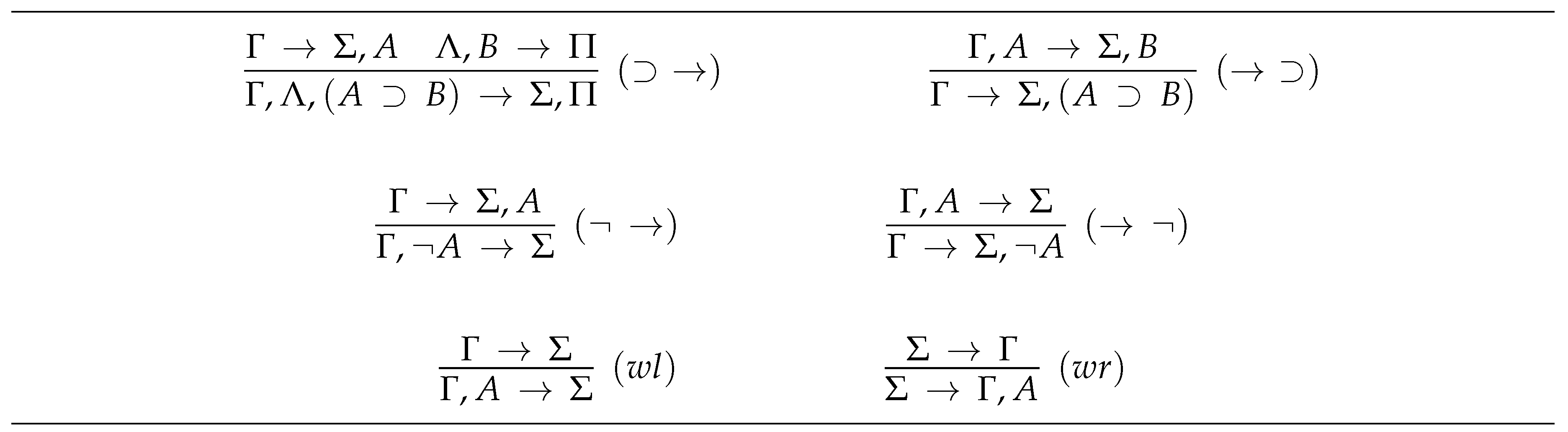
4.1.1. The Sequent Calculus $\mathsf{LK}$

Definition 9.

A (classical) sequent is an ordered pair of the form $\Gamma \to \Sigma$, where Γ and Σ are finite sets of formulas. Γ is the antecedent and Σ is the succedent of the sequent.

For a two-valued interpretation I, a sequent $\Gamma \to \Delta$ is true under I if, whenever all formulas in Γ are true under I, then at least one formula in Δ is true under I. Furthermore, a sequent is valid if it is true under each interpretation.

Following customs, we write sequents of the form $\Gamma \cup \left\{A\right\}\to \Delta$ simply as “$\Gamma ,A\to \Delta$”, and if the antecedent or succedent of a sequent is the empty set, then it is omitted from the sequent.

Definition 10.

The postulates of $\mathsf{LK}$ are as follows:

• axioms of $\mathsf{LK}$ are sequents of the form

  -

  $\to \mathsf{\top }$,

  -

  $\mathsf{\perp }\to$, and

  -

  $A\to A$, where A is a formula;

  and
• the inference rules of $\mathsf{LK}$ are those given in Figure 5.

Note that the last two rules in Figure 5 are the weakening rules of $\mathsf{LK}$. Moreover, from the rules of $\mathsf{LK}$, we can easily obtain derived rules for the defined connectives $\wedge$, $\vee$, and $\equiv$. For instance, the derived rules for $\wedge$ are as follows:

Soundness and completeness of $\mathsf{LK}$ is well known:

Figure 5. Rules of the sequent calculus $\mathsf{LK}$.

Figure 5. Rules of the sequent calculus $\mathsf{LK}$.

Proposition 6

([23]).A sequent $\Gamma \to \Sigma$ is valid iff it is provable in $\mathsf{LK}$.

In particular, the following relation follows immediately:

Corollary 2.

For every formula A,

$${\models }_{2}A\hspace{0.17em}iff\hspace{0.17em}the\hspace{0.17em}sequent\to A\hspace{0.17em}is\hspace{0.17em}provable\hspace{0.17em}in\hspace{0.17em}\mathsf{LK}.$$

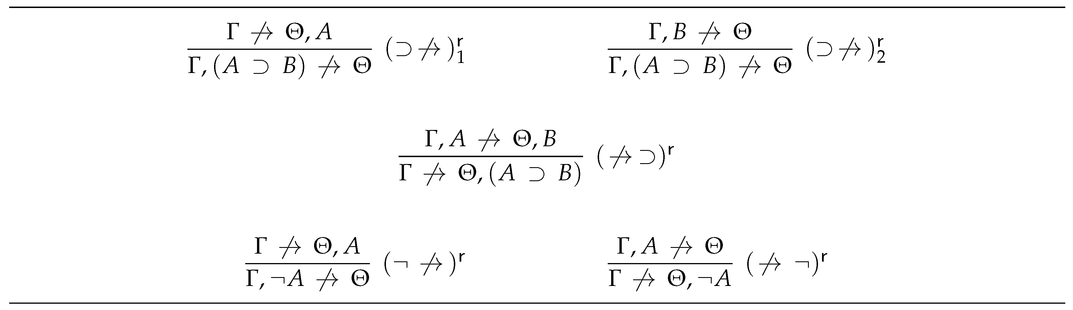
4.1.2. The Anti-Sequent Calculus ${\mathsf{LK}}^{\mathsf{r}}$

Now we introduce our complementary calculus ${\mathsf{LK}}^{\mathsf{r}}$ for axiomatising invalidity in propositional logic, following Bonatti [37] (and Goranko [38]).

Definition 11.

An anti-sequent is an ordered pair of the form $\Gamma \nrightarrow \Theta$, where Γ and Θ are finite sequences of formulas.

For a two-valued interpretation I, an anti-sequent $\Gamma \nrightarrow \Theta$ is refuted by I, or I refutes $\Gamma \nrightarrow \Theta$, if every formula in Γ is true under I and every formula in Θ is false under I. An anti-sequent $\Gamma \nrightarrow \Theta$ is refutable if there is at least one interpretation that refutes $\Gamma \nrightarrow \Theta$.

Hence, the anti-sequent $\Gamma \nrightarrow \Theta$ is refutable iff the classical sequent $\Gamma \to \Theta$ is invalid. Also, in accordance to the convention for classical sequents, we write “$\nrightarrow \Theta$” and “$\Gamma \nrightarrow$” whenever $\Gamma$ or $\Theta$ is the empty set.

Definition 12.

The postulates of ${\mathsf{LK}}^{\mathsf{r}}$ are as follows:

• the axioms of ${\mathsf{LK}}^{\mathsf{r}}$ are anti-sequents of the form $\mathsf{\Phi }\nrightarrow \mathsf{\Psi }$, where Φ and Ψ are disjoint finite sets of atomic formulas such that $\mathsf{\perp }\notin \mathsf{\Phi }$ and $\mathsf{\top }\notin \mathsf{\Psi }$; and
• the inference rules of ${\mathsf{LK}}^{\mathsf{r}}$ are those depicted in Figure 6.

Note that, following the general pattern of complementary calculi, the inference rules of ${\mathsf{LK}}^{\mathsf{r}}$ have only single premisses.

We again can obtain corresponding derived rules for the defined connectives. Below we give the ones for $\wedge$:

Soundness and completeness for ${\mathsf{LK}}^{\mathsf{r}}$ was shown by Bonatti [37] (and, independently, by Goranko [38]):

Proposition 7.

An anti-sequent $\Gamma \nrightarrow \Theta$ is refutable iff it is provable in ${\mathsf{LK}}^{\mathsf{r}}$.

For formulas, we have then the following immediate corollary:

Corollary 3.

For every formula A,

$$/{\models }_{2}A\hspace{0.17em}iff\hspace{0.17em}the\hspace{0.17em}anti-sequent\nrightarrow A\hspace{0.17em}is\hspace{0.17em}provable\hspace{0.17em}in\hspace{0.17em}{\mathsf{LK}}^{\mathsf{r}}.$$

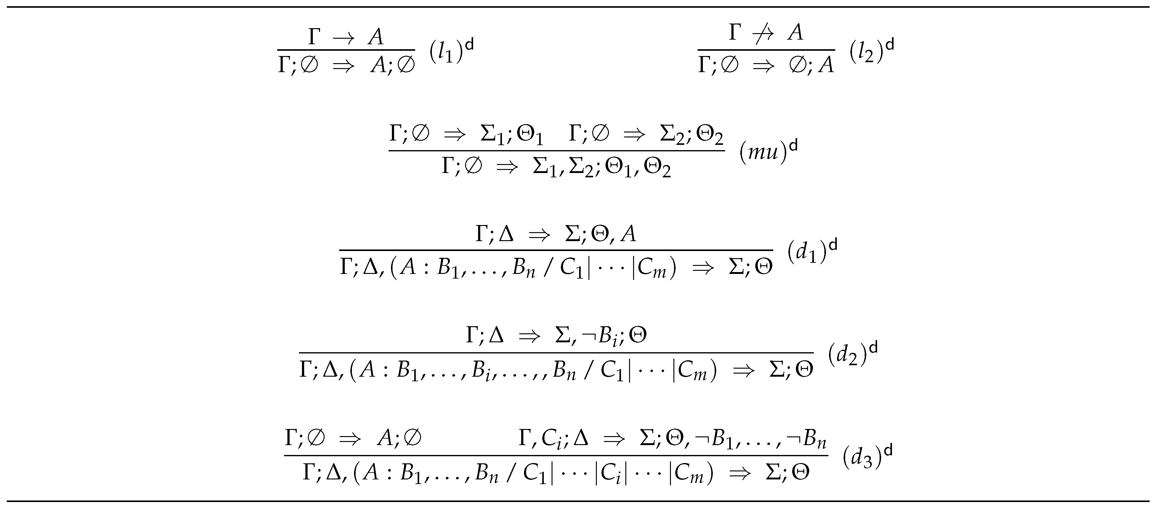
4.1.3. The Default-Sequent Calculus ${\mathsf{B}}_{\mathsf{D}}$

We can now specify our calculus ${\mathsf{B}}_{\mathsf{D}}$ for brave reasoning in disjunctive default logic.

Definition 13.

By a (brave) disjunctive default sequent we understand an ordered quadruple of the form $\Gamma ;\Delta \Rightarrow \Sigma ;\Theta$, where Γ, Σ, and Θ are finite sets of formulas and Δ is a finite set of disjunctive defaults.

A disjunctive default sequent $\Gamma ;\Delta \Rightarrow \Sigma ;\Theta$ is true iff there is an extension E of the disjunctive default theory $\langle \Gamma ,\Delta \rangle$ such that $\Sigma \subseteq E$ and $\Theta \cap E=\varnothing$; E is called a witness of $\Gamma ;\Delta \Rightarrow \Sigma ;\Theta$.

The default sequent calculus ${\mathsf{B}}_{\mathsf{D}}$ consists of sequents, anti-sequents, and disjunctive default sequents. It incorporates the systems $\mathsf{LK}$ for sequents and ${\mathsf{LK}}^{\mathsf{r}}$ for anti-sequents, as well as additional axioms and inference rules for disjunctive default sequents, similar to the case of ${\mathsf{B}}_3$.

Definition 14.

The postulates of ${\mathsf{B}}_{\mathsf{D}}$ comprise the following items:

• all axioms and inference rules of $\mathsf{LK}$ and ${\mathsf{LK}}^{\mathsf{r}}$;
• axioms of the form $\Gamma ;\varnothing \Rightarrow \varnothing ;\varnothing$, where Γ is a finite set of formulas of $\mathbf{PL}$; and
• the inference rules are those depicted in Figure 7.

The informal meaning of the nonmonotonic inference rules is similar to the meaning of the rules in ${\mathsf{B}}_3$:

(i)

rules ${\left(l_1\right)}^{\mathsf{d}}$ and ${\left(l_2\right)}^{\mathsf{d}}$ combine classical sequents and anti-sequents with disjunctive default sequents, respectively;

(ii)

rule ${\left(\mathit{mu}\right)}^{\mathsf{d}}$ again allows the joining of information in case that no default is present; and

(iii)

rules ${\left(d_1\right)}^{\mathsf{d}}$, ${\left(d_2\right)}^{\mathsf{d}}$, and ${\left(d_3\right)}^{\mathsf{d}}$ are the default introduction rules, where rules ${\left(d_1\right)}^{\mathsf{d}}$ and ${\left(d_2\right)}^{\mathsf{d}}$ take care of introducing non-active defaults, whilst rule ${\left(d_3\right)}^{\mathsf{d}}$ allows to introduce an active default.

Before we turn to the adequacy of ${\mathsf{B}}_{\mathsf{D}}$, let us again give an example to illustrate the calculus.

Example 6.

Let us consider the disjunctive default theory from Example 4 dealing with Poole’s broken arms scenario [52], which contains the defaults

$$\frac{:U_l\wedge \neg B_l}{U_l}and\frac{:U_r\wedge \neg B_l}{U_r},$$

together with the disjunctive default

$$B_l|B_r.$$

This disjunctive default theory has the two extensions:

$${\mathrm{Th}}_2\left(\{B_l,U_r\}\right)and{\mathrm{Th}}_2\left(\{B_r,U_l\}\right).$$

Accordingly, the following disjunctive default sequent is true:

$$\varnothing ;(:\varnothing /{\mathit{B}}_{\mathit{l}}|{\mathit{B}}_{\mathit{r}}),(:({\mathit{U}}_{\mathit{l}}\wedge \neg {\mathit{B}}_{\mathit{l}})/{\mathit{U}}_{\mathit{l}}),(:({\mathit{U}}_{\mathit{r}}\wedge \neg {\mathit{B}}_{\mathit{r}})/{\mathit{U}}_{\mathit{r}})\Rightarrow {\mathit{B}}_{\mathit{l}},{\mathit{U}}_{\mathit{r}},\neg ({\mathit{U}}_{\mathit{l}}\wedge \neg {\mathit{B}}_{\mathit{l}});{\mathit{U}}_{\mathit{l}}.$$

A proof, γ, of this sequent in ${\mathsf{B}}_{\mathsf{D}}$ is given below; it uses the two subproofs α and β:

• Proof α:
• Proof β:
• Proof γ:

4.2. Adequacy of the Calculus

Soundness and completeness of ${\mathsf{B}}_{\mathsf{D}}$ can be shown by similar arguments as in the case of ${\mathsf{B}}_3$. We sketch the relevant details.

We again need some preparatory characterisations of extensions, dealing with the introduction of active or non-active defaults.

We start with the notion of a reduct, adapted to the case of ${\mathbf{DL}}_{\mathbf{D}}$, as introduced by Gelfond, Lifschitz, Przymusinska, and Truszczyński [10].

In what follows, we use the following terminology: By a disjunctive inference rule, or simply a disjunctive rule, r, we understand an expression of the form

$$\frac{A}{C_1|\cdots |C_m}.$$

We say that a set S of formulas is closed under r if, whenever $A\in S$, then $C_i\in S$, for some $i\in \{1,\dots ,m\}$. Moreover, for a set R of disjunctive rules, we say that S is closed under R if S is closed under each $r\in R$.

Definition 15.

Let D be a set of disjunctive defaults and E a set of formulas. The ${\mathbf{DL}}_{\mathbf{D}}$-reduct of D with respect to E, denoted by $D_E^{\mathsf{d}}$, is the set consisting of the following disjunctive inference rules:

$$\begin{array}{cc}\hfill D_E^{\mathsf{d}}:=& {\displaystyle \left.\left\{\frac{A}{C_1|\cdots |C_m}\right|\frac{A:B_1,\dots ,B_n}{C_1|\cdots |C_m}\in D\hspace{0.17em}and\{\neg B_1,\dots ,\neg B_n\}\cap E=\varnothing \right\}.}\hfill \end{array}$$

A disjunctive rule

$$\frac{A}{C_1|\cdots |C_m}$$

is called ${\mathbf{DL}}_{\mathbf{D}}$-residue of a default

$$\frac{A:B_1,\dots ,B_n}{C_1|\cdots |C_m}.$$

We again allow ourselves to drop the prefix “${\mathbf{DL}}_{\mathbf{D}}$-” from “${\mathbf{DL}}_{\mathbf{D}}$-reduct” and “${\mathbf{DL}}_{\mathbf{D}}$-residue” if no ambiguity can arise.

Towards our characterisation of extensions of disjunctive default theories, we introduce the following notation:

Definition 16.

For a set W of formulas and a set R of disjunctive rules, let $C^R\left(W\right)$ be the collection of all sets which

(i) 

contain W,

(ii) 

are closed under propositional consequence, and

(iii) 

are closed under R.

Furthermore, let ${\mathit{Cn}}^R\left(W\right)=min\left(C^R\left(W\right)\right)$, i.e., ${\mathit{Cn}}^R\left(W\right)$ contains all minimal sets satisfying (i)–(iii).

Note that, for a disjunctive default theory $T=\langle W,D\rangle$ and a set E of formulas, we obviously have that:

$${\mathit{Cl}}_T\left(E\right)=C^{D_E^{\mathsf{d}}}\left(W\right)\mathrm{and}{\Delta }_T\left(E\right)=C{n}^{D_E^{\mathsf{d}}}\left(W\right).$$

From this, the following result is immediate:

Theorem 7.

Let $T=\langle W,D\rangle$ be a disjunctive default theory. Then,

$$E\hspace{0.17em}is\hspace{0.17em}an\hspace{0.17em}extension\hspace{0.17em}T\hspace{0.17em}iff\hspace{0.17em}E\in {\mathit{Cn}}^{D_E^{\mathsf{d}}}\left(W\right)$$

.

Note furthermore that, if $T=\langle W,D\rangle$ is a standard default theory, i.e., if D contains no proper disjunctive defaults, then clearly ${\mathit{Cn}}^{D_E^{\mathsf{d}}}\left(W\right)=\left\{{\mathrm{Th}}_2^{D_E^{\mathsf{d}}}\left(W\right)\right\}$ and E is an extension in the standard default logic sense iff $E={\mathrm{Th}}_2^{D_E^{\mathsf{d}}}\left(W\right)$, where ${\mathrm{Th}}_2^{D_E^{\mathsf{d}}}\left(W\right)$ is the deductive closure operator of classical derivability extended by the (standard) inference rules in $D_E^{\mathsf{d}}$.

We continue with the following pendant to activeness as defined earlier:

Definition 17.

Let E be a set of formulas. A disjunctive default

$$\frac{A:B_1,\dots ,B_n}{C_1|\cdots |C_m}$$

is active in E iff $E⊢A$ and $\{\neg B_1,\dots ,\neg B_n\}\cap E=\varnothing$.

We again employ our notation $\mathsf{p}\left(d\right)$ as in case of ${\mathbf{DL}}_{\mathbf{3}}$, but now we define and $\mathsf{j}\left(d\right)$ for a default d, but now we define

$${\mathsf{j}}^{\prime }\left(d\right):=\{B_1,\dots ,B_n\}\mathrm{and}{\mathsf{c}}^{\prime }\left(d\right):=\{C_1,\dots ,C_m\},$$

for $d=(A:B_1,\dots ,B_n/C_1|\cdots \left|C_m\right)$.

We obtain the following results corresponding to Lemma 2 and Theorems 2–4, respectively:

Lemma 3.

Let W and E be sets of formulas, R a set of disjunctive inference rules, and

$$r=\frac{A}{B_1|\cdots |B_n}$$

a disjunctive inference rule. Then:

1. 

If $A\notin E$ and $E\in {\mathit{Cn}}^R\left(W\right)$, then $E\in {\mathit{Cn}}^{R\cup \left\{r\right\}}\left(W\right)$.

2. 

If $A\in E$ and $E\in {\mathit{Cn}}^{R\cup \left\{r\right\}}\left(W\right)$, then $E\in {\mathit{Cn}}^R(W\cup \left\{B\right\})$, for some formula $B\in \{B_1,\dots ,B_n\}$.

Theorem 8.

Let $T=\langle W,D\rangle$ be a disjunctive default theory, E a set of formulas, and d a disjunctive default not active in E. Then, E is an extension of $\langle W,D\rangle$ iff E is an extension of $\langle W,D\cup \left\{d\right\}\rangle$.

Theorem 9.

Let E be a set of formulas and d a disjunctive default.

1. 

If E is an extension of $\langle W,D\cup \left\{d\right\}\rangle$ and d is active in E, then E is an extension of $\langle W\cup \left\{C\right\},D\rangle$, for some $C\in {\mathsf{c}}^{\prime }\left(d\right)$.

2. 

If E is an extension of the disjunctive default theory $\langle W\cup \left\{C\right\},D\rangle$, for some $C\in {\mathsf{c}}^{\prime }\left(d\right)$, $W⊢\mathsf{p}\left(d\right)$, and $\neg {\mathsf{j}}^{\prime }\left(d\right)\cap E=\varnothing$, then E is an extension of $\langle W,D\cup \left\{d\right\}\rangle$.

From this, by similar arguments as in the case of ${\mathsf{B}}_3$, soundness and completeness of ${\mathsf{B}}_{\mathsf{D}}$ follows.

Theorem 10.

A disjunctive default sequent $\Gamma ;\Delta \Rightarrow \Sigma ;\Theta$ is provable in ${\mathsf{B}}_{\mathsf{D}}$ iff it is true.

5. Conclusions

In this paper, we introduced sequent-type calculi for brave reasoning for a three-valued version of default logic [9] and for disjunctive default logic [10], following the method of Bonatti [7]. This form of axiomatisation yielded a particular elegant formulation mainly due to their usage of anti-sequents. In addition, the approach was flexible and could be applied to formalise different versions of nonmonotonic reasoning. Indeed, other variants of default logic besides the versions studied here, including justified default logic [12] and constrained default logic [13,14], have also been axiomatised by this sequent method [60,61].

Related to the sequent approach discussed here are also works employing tableau methods. In particular, Niemelä [62] introduces a tableau calculus for inference under circumscription. Other tableau approaches, however, do not encode inference directly, rather they characterise models (resp., extensions) associated with a particular nonmonotonic reasoning formalism [63,64,65,66].

Variations of our calculi can be obtained by using different calculi for the underlying monotonic logics. As far as the three-valued case is concerned, we opted for the style of calculi as discussed by Rousseau [25] and Zach [26] because they naturally model the underlying semantic conditions of the considered logic. Alternatively, we could have also used two-sided sequent and anti-sequent calculi like the ones described by Avron [24] and Oetsch and Tompits [67], respectively. By employing such two-sided sequents, however, one then deals with calculi having also “non-standard” inference rules introducing two connectives simultaneously. Another prominent proof method for many-valued logics are hypersequent calculi [57], which are basically disjunctions of two-sided sequents. However, to the best of our knowledge, no rejection calculus based on hypersequents exist so far and establishing such a system in particular for ${\mathsf{Ł}}_{\mathbf{3}}$ would be worthwhile.

Another topic for future work is to develop calculi for sceptical reasoning for the considered versions of default logic as well as for other variants of default logic discussed in the literature [12,13,14], similar to the system for sceptical reasoning for standard default logic as introduced by Bonatti and Olivetti [8]. In that work, they also introduced a different version of a calculus for brave default reasoning—extending this calculus to ${\mathbf{DL}}_{\mathbf{3}}$ and ${\mathbf{DL}}_{\mathbf{D}}$ would provide an alternative to the calculi discussed here.

References

- Reiter, R. A Logic for Default Reasoning. Artif. Intell. 1980, 13, 81–132. [Google Scholar] [CrossRef]
- Moore, R.C. Semantical Considerations on Nonmonotonic Logic. Artif. Intell. 1985, 25, 75–94. [Google Scholar] [CrossRef]
- McCarthy, J. Circumscription—A Form of Non-Monotonic Reasoning. Artif. Intell. 1980, 13, 27–39. [Google Scholar] [CrossRef]
- Gelfond, M.; Lifschitz, V. Classical Negation in Logic Programs and Disjunctive Databases. New Gener. Comput. 1991, 9, 365–385. [Google Scholar] [CrossRef]
- Pearce, D. Equilibrium Logic. Ann. Math. Artif. Intell. 2006, 47, 3–41. [Google Scholar] [CrossRef]
- Minsky, M. A Framework for Representing Knowledge. In Mind Design; Haugeland, J., Ed.; MIT Press: Cambridge, MA, USA, 1975; pp. 95–128. [Google Scholar]
- Bonatti, P.A. Sequent Calculi for Default and Autoepistemic Logic. In Proceedings of the 5th International Workshop on Theorem Proving with Analytic Tableaux and Related Methods (TABLEAUX ’96), Lecture Notes in Computer Science, Terrasini, Palermo, Italy, 15–17 May 1996; Miglioli, P., Moscato, U., Mundici, D., Ornaghi, M., Eds.; Springer: Berlin/Heidelberg, Germany, 1996; Volume 1071, pp. 127–142. [Google Scholar]
- Bonatti, P.A.; Olivetti, N. Sequent Calculi for Propositional Nonmonotonic Logics. ACM Trans. Comput. Log. 2002, 3, 226–278. [Google Scholar] [CrossRef]
- Radzikowska, A. A Three-Valued Approach to Default Logic. J. Appl. Non-Class. Logics 1996, 6, 149–190. [Google Scholar] [CrossRef]
- Gelfond, M.; Lifschitz, V.; Przymusinska, H.; Truszczyński, M. Disjunctive Defaults. In Proceedings of the 2nd International Conference on Principles of Knowledge Representation and Reasoning (KR’91), Cambridge, MA, USA, 22–25 April 1991; Allen, J.F., Fikes, R., Sandewall, E., Eds.; Morgan Kaufmann: Burlington, MA, USA, 1991; pp. 230–237. [Google Scholar]
- Łukasiewicz, J. Philosophische Bemerkungen zu mehrwertigen Systemen des Aussagenkalküls. Comptes Rendus Des Séances De La Société Des Sciences Et Des Lettres De Varsovie Cl III 1930, 23, 51–77. [Google Scholar]
- Łukaszewicz, W. Considerations on Default Logic—An alternative approach. Comput. Intell. 1988, 4, 1–16. [Google Scholar] [CrossRef]
- Schaub, T. On Constrained Default Theories; Technical Report AIDA-92-2; FG Intellektik, FB Informatik, TH Darmstadt: Darmstadt, Germany, 1992. [Google Scholar]
- Delgrande, J.P.; Schaub, T.; Jackson, W.K. Alternative Approaches to Default Logic. Artif. Intell. 1994, 70, 167–237. [Google Scholar] [CrossRef]
- Mikitiuk, A.; Truszczyński, M. Rational Default Logic and Disjunctive Logic Programming. In Proceedings of the 2nd International Workshop on Logic Programming and Non-Monotonic Reasoning (LPNMR’93), Lisbon, Portugal, 28–30 June 1993; Pereira, L.M., Nerode, A., Eds.; MIT Press: Cambridge, MA, USA, 1993; pp. 283–299. [Google Scholar]
- Zhou, Y.; Lin, F.; Zhang, Y. General Default Logic. Ann. Math. Artif. Intell. 2009, 57, 125–160. [Google Scholar] [CrossRef]
- Yue, A.; Ma, Y.; Lin, Z. Four-Valued Semantics for Default Logic. In Proceedings of the 19th Conference of the Canadian Society for Computational Studies of Intelligence (Canadian AI 2006), Lecture Notes in Computer Science, Quebec City, QC, Canada, 7–9 June 2006; Lamontagne, L., Marchand, M., Eds.; Springer: Berlin/Heidelberg, Germany, 2006; Volume 4013, pp. 195–205. [Google Scholar]
- Antoniou, G.; Wang, K. Default Logic. In Handbook of the History of Logic, Volume 8: The Many Valued and Nonmonotonic Turn in Logic; Gabbay, D., Woods, J., Eds.; North-Holland: Amsterdam, The Netherlands, 2007; pp. 517–632. [Google Scholar]
- Beyersdorff, O.; Meier, A.; Thomas, M.; Vollmer, H. The Complexity of Reasoning for Fragments of Default Logic. J. Log. Comput. 2012, 22, 587–604. [Google Scholar] [CrossRef]
- Łukasiewicz, J. O sylogistyce Arystotelesa. Sprawozdania Z Czynności I Posiedzeń Polskiej Akademii Umiejętności 1939, 44, 220–226. [Google Scholar]
- Béziau, J.Y. A Sequent Calculus for Lukasiewicz’s Three-Valued Logic Based on Suszko’s Bivalent Semantics. Bull. Sect. Log. 1999, 28, 89–97. [Google Scholar]
- Avron, A. Classical Gentzen-Type Methods in Propositional Many-Valued Logics. In Beyond Two: Theory and Applications in Multiple-Valued Logics; Fitting, M., Orłowska, E., Eds.; Springer: Berlin/Heidelberg, Germany, 2003; pp. 117–155. [Google Scholar]
- Gentzen, G. Untersuchungen über das logische Schließen I. Math. Z. 1935, 39, 176–210. [Google Scholar] [CrossRef]
- Avron, A. Natural 3-Valued Logics—Characterization and Proof Theory. J. Symb. Log. 1991, 56, 276–294. [Google Scholar] [CrossRef]
- Rousseau, G.S. Sequents in Many Valued Logic I. Fundam. Math. 1967, 60, 23–33. [Google Scholar] [CrossRef][Green Version]
- Zach, R. Proof Theory of Finite-Valued Logics. Master’s Thesis, Technische Universität Wien, Institut für Computersprachen, Wien, Austria, 1993. [Google Scholar]
- Bogojeski, M.; Tompits, H. On Sequent-Type Rejection Calculi for Many-Valued Logics. In Reasoning: Games, Cognition, Logic; Urbański, M., Skura, T., Łupkowski, P., Eds.; College Publications: London, UK, 2020; pp. 193–207. [Google Scholar]
- Łukasiewicz, J. Logika dwuwartościowa. Przegląd Filozoficzny 1921, 23, 189–205. [Google Scholar]
- Łukasiewicz, J. Aristotle’s Syllogistic from the Standpoint of Modern Formal Logic, 2nd ed.; Clarendon Press: Oxford, UK, 1957. [Google Scholar]
- Słupecki, J. Z Badań Nad Sylogistyką Arystotelesa; Wrocławskie Towarzystwo Naukowe: Wrocław, Poland, 1948; Volume 6, pp. 1–30. [Google Scholar]
- Słupecki, J. Funkcja Łukasiewieza. Zesz. Nauk. Uniw. Wrocławskiego Ser. A 1959, 3, 33–40. [Google Scholar]
- Wybraniec-Skardowska, U. Teoria zdań odrzuconych. Zesz. Nauk. Wyższej Szkoły Pedagog. W Opolu Ser. B Stud. I Monogr. 1969, 22, 5–131. [Google Scholar]
- Bryll, G. Kilka uzupelnień teorii zdań odrzuconych. Zesz. Nauk. Wyższej Szkoły Pedagog. W Opolu Ser. B Stud. I Monogr. 1969, 22, 133–154. [Google Scholar]
- Słupecki, J.; Bryll, G.; Wybraniec-Skardowska, U. Theory of Rejected Propositions I. Stud. Log. 1971, 29, 75–115. [Google Scholar] [CrossRef]
- Słupecki, J.; Bryll, G.; Wybraniec-Skardowska, U. Theory of Rejected Propositions II. Stud. Log. 1972, 30, 97–139. [Google Scholar] [CrossRef]
- Tiomkin, M.L. Proving Unprovability. In Proceedings of the Third Annual Symposium on Logic in Computer Science (LICS’88), Scotland, UK, 5–8 July 1988; IEEE Computer Society: Washington, DC, USA, 1988; pp. 22–26. [Google Scholar]
- Bonatti, P.A. A Gentzen System for Non-Theorems; Technical Report CD-TR 93/52; Christian Doppler Labor für Expertensysteme, Technische Universität Wien: Vienna, Austria, 1993. [Google Scholar]
- Goranko, V. Refutation Systems in Modal Logic. Stud. Log. 1994, 53, 299–324. [Google Scholar] [CrossRef]
- Skura, T. A Complete Syntactic Characterization of the Intuitionistic Logic. Rep. Math. Log. 1989, 23, 75–80. [Google Scholar]
- Dutkiewicz, R. The Method of Axiomatic Rejection for the Intuitionistic Propositional Logic. Stud. Log. 1989, 48, 449–459. [Google Scholar] [CrossRef]
- Pinto, L.; Dyckhoff, R. Loop-Free Construction of Counter-Models for Intuitionistic Propositional Logic. In Symposia Gaussiana, Proceedings of the 2nd Gauss Symposium, Conference A: Mathematics and Theoretical Physics, Munich, Germany, 2–7 August 1993; Behara, M., Fritsch, R., Lintz, R.G., Eds.; Walter de Gruyter: Berlin, Germany, 1995; pp. 225–232. [Google Scholar]
- Skura, T. Aspects of Refutation Procedures in the Intuitionistic Logic and Related Modal Systems. Acta Univ. Wratislav. Log. 1999, 20, 1–84. [Google Scholar]
- Skura, T. Refutation Systems in Propositional Logic. In Handbook of Philosophical Logic, 2nd ed.; Gabbay, D., Guenthner, D., Eds.; Springer: Berlin/Heidelberg, Germany, 2011; Volume 16, pp. 115–157. [Google Scholar]
- Skura, T. Refutation Methods in Modal Propositional Logic; Semper: Warszawa, Poland, 2013. [Google Scholar]
- Berger, G.; Tompits, H. On Axiomatic Rejection for the Description Logic . In Declarative Programming and Knowledge Management–Declarative Programming Days (KDPD 2013); Revised Selected Papers; Lecture Notes in Computer Science; Springer: Cham, Switzerland, 2014; Volume 8439, pp. 65–82. [Google Scholar]
- Wybraniec-Skardowska, U. On the Notion and Function of the Rejection of Propositions. Acta Univ. Wratislav. Log. 2005, 23, 179–202. [Google Scholar]
- Rosser, J.B.; Turquette, A.R. Many-Valued Logics; North-Holland: Amsterdam, The Netherlands, 1952. [Google Scholar]
- Malinowski, G. Many-Valued Logic and its Philosophy. In Handbook of the History of Logic, Volume 8: The Many Valued and Nonmonotonic Turn in Logic; Gabbay, D., Woods, J., Eds.; North-Holland: Amsterdam, The Netherlands, 2007; pp. 13–94. [Google Scholar]
- Wajsberg, M. Aksjomatyzacja trójwartościowego rachunku zdań. Comptes Rendus Des Séances De La Société Des Sciences Et Des Lettres De Varsovie Cl III 1931, 24, 136–148. [Google Scholar]
- Łukaszewicz, W. Non-Monotonic Reasoning: Formalization of Commonsense Reasoning; Ellis Horwood: Chichester, UK, 1990. [Google Scholar]
- Pearl, J. Probabilistic Reasoning in Intelligent Systems: Networks of Plausible Inference; Morgan Kaufmann Publishers: Burlington, MA, USA, 1988. [Google Scholar]
- Poole, D. What the Lottery Paradox Tells us about Default Reasoning. In Proceedings of the First International Conference on Principles of Knowledge Representation and Reasoning (KR’89), Toronto, ON, Canada, 15–18 May 1989; Brachman, R.J., Levesque, H.J., Reiter, R., Eds.; Morgan Kaufmann: Burlington, MA, USA, 1989; pp. 333–340. [Google Scholar]
- Lin, F.; Shoham, Y. Epistemic Semantics for Fixed-Points Non-Monotonic Logics. In Proceedings of the Third Conference on Theoretical Aspects of Reasoning about Knowledge (TARK’90), Pacific Grove, CA, USA, 4–7 March 1990; Parikh, R., Ed.; Morgan Kaufmann: Burlington, MA, USA, 1990; pp. 111–120. [Google Scholar]
- Baumgartner, R.; Gottlob, G. Propositional Default Logics Made Easier: Computational Complexity of Model Checking. Theor. Comput. Sci. 2002, 289, 591–627. [Google Scholar] [CrossRef]
- Bonatti, P.A. Sequent Calculi for Default and Autoepistemic Logic; Technical Report CD-TR 93/53; Christian Doppler Labor für Expertensysteme, Technische Universität Wien: Wien, Austria, 1993. [Google Scholar]
- Carnielli, W.A. On Sequents and Tableaux for Many-Valued Logics. J. Non-Class. Log. 1991, 8, 59–76. [Google Scholar]
- Avron, A. The Method of Hypersequents in the Proof Theory of Propositional Non-Classical Logics. In Logic: From Foundations to Applications; Clarendon Press: Oxford, UK, 1996; pp. 1–32. [Google Scholar]
- Hähnle, R. Tableaux for Many-Valued Logics. In Handbook of Tableaux Methods; D’Agostino, M., Gabbay, D., Hähnle, R., Posegga, J., Eds.; Kluwer: Dordrecht, The Netherlands, 1999; pp. 529–580. [Google Scholar]
- Marek, W.; Truszczyński, M. Nonmonotonic Logic: Context-Dependent Reasoning; Springer: Berlin/Heidelberg, Germany, 1993. [Google Scholar]
- Egly, U.; Tompits, H. A Sequent Calculus for Intuitionistic Default Logic. In Proceedings of the 12th Workshop on Logic Programming (WLP’97), Forschungsbericht PMS-FB-1997-10, Institut für Informatik, Ludwig-Maximilians-Universität München, Munich, Germany, 17–19 September 1997; pp. 69–79. [Google Scholar]
- Lupea, M. Axiomatization of Credulous Reasoning in Default Logics using Sequent Calculus. In Proceedings of the 10th International Symposium on Symbolic and Numeric Algorithms for Scientific Computing (SYNASC 2008), Timisoara, Romania, 26–29 September 2008. [Google Scholar]
- Niemelä, I. Implementing Circumscription Using a Tableau Method. In Proceedings of the 12th European Conference on Artificial Intelligence (ECAI’96), Budapest, Hungary, 11–16 August 1996; Wahlster, W., Ed.; John Wiley and Sons: New York, NY, USA, 1996; pp. 80–84. [Google Scholar]
- Amati, G.; Aiello, L.C.; Gabbay, D.; Pirri, F. A Proof Theoretical Approach to Default Reasoning I: Tableaux for Default Logic. J. Log. Comput. 1996, 6, 205–231. [Google Scholar] [CrossRef][Green Version]
- Pearce, D.; de Guzmán, I.P.; Valverde, A. A Tableau Calculus for Equilibrium Entailment. In Proceedings of the 9th International Conference on Automated Reasoning with Analytic Tableaux and Related Methods (TABLEAUX 2000), Lecture Notes in Computer Science, St Scotland, UK, 3–7 July 2000; Dyckhoff, R., Ed.; Springer: Berlin/Heidelberg, Germany, 2000; Volume 1847, pp. 352–367. [Google Scholar]
- Cabalar, P.; Odintsov, S.P.; Pearce, D.; Valverde, A. Partial Equilibrium Logic. Ann. Math. Artif. Intell. 2007, 50, 305–331. [Google Scholar] [CrossRef][Green Version]
- Gebser, M.; Schaub, T. Tableau Calculi for Logic Programs under Answer Set Semantics. ACM Trans. Comput. Log. 2013, 14, 1–40. [Google Scholar] [CrossRef]
- Oetsch, J.; Tompits, H. Gentzen-Type Refutation Systems for Three-Valued Logics with an Application to Disproving Strong Equivalence. In Proceedings of the 11th International Conference on Logic Programming and Nonmonotonic Resoning (LPNMR 2011), Lecture Notes in Computer Science, Vancouver, BC, Canada, 16–19 May 2011; Delgrande, J.P., Faber, W., Eds.; Springer: Berlin/Heidelberg, Germany, 2011; Volume 6645, pp. 254–259. [Google Scholar]
© 2020 by the authors. Licensee MDPI, Basel, Switzerland. This article is an open access article distributed under the terms and conditions of the Creative Commons Attribution (CC BY) license (http://creativecommons.org/licenses/by/4.0/).
Share and Cite
Pkhakadze, S.; Tompits, H. Sequent-Type Calculi for Three-Valued and Disjunctive Default Logic. Axioms 2020, 9, 84. https://doi.org/10.3390/axioms9030084
Pkhakadze S, Tompits H. Sequent-Type Calculi for Three-Valued and Disjunctive Default Logic. Axioms. 2020; 9(3):84. https://doi.org/10.3390/axioms9030084
Chicago/Turabian StylePkhakadze, Sopo, and Hans Tompits. 2020. "Sequent-Type Calculi for Three-Valued and Disjunctive Default Logic" Axioms 9, no. 3: 84. https://doi.org/10.3390/axioms9030084
APA StylePkhakadze, S., & Tompits, H. (2020). Sequent-Type Calculi for Three-Valued and Disjunctive Default Logic. Axioms, 9(3), 84. https://doi.org/10.3390/axioms9030084