Abstract
Boundary value problems having fractional derivative in space are used in several fields, like biology, mechanical engineering, control theory, just to cite a few. In this paper we present a new numerical method for the solution of boundary value problems having Caputo derivative in space. We approximate the solution by the Schoenberg-Bernstein operator, which is a spline positive operator having shape-preserving properties. The unknown coefficients of the approximating operator are determined by a collocation method whose collocation matrices can be constructed efficiently by explicit formulas. The numerical experiments we conducted show that the proposed method is efficient and accurate.
1. Introduction
Boundary value problems having fractional derivative in space are used to describe physical phenomena in which nonlocality effect are peculiar. For instance, they are used to model anomalous diffusion in biological tissues, viscoplastic materials in mechanical engineering or control of dynamical systems (see References [1,2,3,4,5] and references therein).
In particular, in this paper we are concerned with the Caputo fractional derivative [6]. The theoretical analysis of fractional boundary value problems (FBVPs) having Caputo derivative in space was addressed, for instance, in References [6,7,8,9,10,11]. We refer also to References [4,6,12,13] for the foundations of fractional calculus and details on fractional derivatives. We want to mention that in recent years other types of fractional derivatives were introduced, like the He’s derivative [14] or the Fabrizio-Caputo derivative [15]. These derivatives are used to model physical phenomena characterized by the presence of structures with different scales.
In the literature several analytical and numerical methods were proposed for the solution of FBVPs. Analytical methods based on the homotopy perturbation technique [16] and the variational iteration method [17] were used, for instance, in References [18,19,20]. As for the numerical methods, several methods were proposed in the literature. In Reference [21] the authors proposed a Galerkin finite element approach to solve the one-dimensional steady state fractional advection dispersion equation. In Reference [22] the authors used finite difference methods to solve a nonlinear FBVP while in Reference [10] a collocation method based on spline functions was proposed to solve linear FBVPs. Spectral methods based on generalized Jacobi polynomials were used, for instance, in References [23,24]. In Reference [11] a Gegenbauer-based Nyström method was proposed to solve one-dimensional fractional-Laplacian boundary-value problems. In Reference [25] the authors solved linear and nonlinear FBVPs by a wavelet method. For an overview on numerical methods to solve fractional differential problems see, for instance, References [18,20,26,27,28,29,30] and references therein.
In this paper we present a collocation method, based on a spline quasi-interpolant operator, for the solution of boundary value problems having Caputo derivative in space. Quasi-interpolant operators are approximating operators that reproduce polynomials up to a given degree. They have a greater flexibility with respect to interpolation operator. This freedom can be used to preserve special properties of the function to be approximated, like the sign, the shape or the area of its graph [31,32,33,34,35]. In particular, in this paper we propose a numerical method based on the Schoenberg-Bernstein operator [36], which is a positive operator having shape preserving properties. We determine the unknown coefficients of the approximating operator by a collocation method derived from References [37,38] and show through some numerical experiments that the method is efficient and accurate.
The paper is organized as follows. In Section 2 we describe the FBVPs we are interested in and the spline basis we use to construct approximating functions in this space. The main properties of the Schoenberg-Bernstein operator are also recalled. The details on the numerical method we propose are described in Section 3. The results of the numerical experiments are shown in Section 4 while some conclusions are given in Section 5.
2. Materials and Methods
In this section we describe the differential problem we are interested in (Section 2.1), the B-spline basis (Section 2.2, Section 2.3 and Section 2.4) used to construct the approximating function, and the main properties of the Schoenberg-Bernstein operator (Section 2.5).
2.1. Fractional Boundary Value Problems
We consider the one-dimensional boundary value problem
where is a real positive number such that , f and g are continuous known functions, and , , , , are known parameters.
Here, denotes the Caputo fractional derivative in space defined as [6]
where is the Euler’s gamma function
We assume y is a sufficient smooth function and the boundary conditions are linearly independent so that the differential problem has a unique solution [6,39,40].
2.2. The Cardinal B-Splines through the Truncated Power Function
The cardinal B-splines are compactly supported piecewise polynomials having breakpoints at the integers. They can be used to construct a function basis for the spline spaces. For details on spline functions see [41,42].
In this context it is convenient to define the cardinal B-splines by applying the divided difference operator to the truncated power function on the sequence of simple integer knots . Thus, the cardinal B-spline of integer degree has expression
where is the collocation matrix of the function system evaluated on the knots . We notice that the cardinal B-spline is compactly supported on and positive in .
The system of the integer translates forms a basis for the n-degree spline space on the real line. Moreover, it reproduces polynomials up to degree n, has approximation order , and is a partition of unity, that is,
2.3. B-Spline Bases on the Finite Interval
On the finite interval a suitable basis for the spline space is the optimal basis, which is constructed using knots of multiplicity at the endpoints of the interval [41,42].
For the sake of simplicity, we assume L is an integer greater than n. Thus, on the finite interval we consider the sequence of integer knots , where , and
The optimal basis on the interval is formed by basis functions, that is,
where the functions and , , are left and right boundary functions, respectively, while the functions , , are internal functions.
The internal functions are the integer translates having support all contained in the interval , that is,
The analytical expression of the left boundary functions is (cf. [43])
where is the order collocation matrix
and is the order collocation matrix
The analytical expression of the right boundary functions can be obtained using the central symmetry property, that is,
We notice that by construction the following endpoint conditions hold
where denotes the Kronecker symbol.
The optimal basis can be refined by using any sequence of equidistant knots on the interval [41,42]. Denoting by h the refinement step, that is, the distance between the refined knot sequence, the refined basis is
where . Once again, the basis has boundary and internal functions. and , , are the right and left boundary functions, respectively, and , , are the internal functions. We notice that the refinement of the knots increases just the number of the internal functions while the number of the boundary functions remains the same.
The optimal basis for the cubic spline space on the interval with refinement step is displayed in Figure 1.
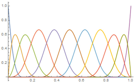
Figure 1.
The optimal basis on the interval with refinement step .
2.4. Fractional Derivatives of Cardinal B-Splines
Since the internal functions are the basis functions having support all contained in the interval , their fractional derivatives can be easily evaluated by the differentiation rule
where
is the backward finite difference operator [37,44]. We notice that the fractional derivatives of the classical polynomial B-splines are fractional splines, that is, splines having noninteger degree (cf. Reference [44]). The fractional derivative of the cubic B-spline, evaluated for different values of , is shown in Figure 2. The plots show that the shape of the fractional derivative varies continuously with so that the order of the derivative acts as a tension parameter.
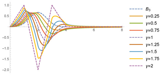
Figure 2.
The fractional derivative of the cubic B-spline for different values of the fractional order . The cubic B-spline , its first () and second () derivatives are plotted as dashed lines.
The explicit expression of the fractional derivative of the left boundary functions can be obtained by applying the fractional differentiation operator to their analytical expression (5) (cf. Reference [43]), that is,
where
The fractional derivative of the right boundary functions can be obtained by the symmetry property, that is,
Thus, the fractional derivative of the boundary functions is a linear combination of the fractional derivative of the translates of the truncated power function whose derivative has expression [43]
where , and denotes the rising Pochhammer symbol.
The fractional derivatives of the boundary functions of the cubic B-spline basis , evaluated for different values of , are shown in Figure 3.
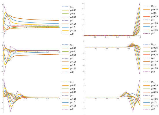
Figure 3.
The fractional derivative of the left boundary functions (left panels) and of the right boundary functions (right panels) of the cubic B-spline basis for different values of the fractional order . The boundary functions and their first () and second () derivatives are plotted as dashed lines.
2.5. The Schoenberg-Bernstein Operator
A spline quasi-interpolant operator is a spline approximation of a given function that reproduces polynomials up to a given degree. There are several types of quasi-interpolant operators depending on which properties of the function to be approximated we require to preserve (see, for instance, References [31,32,33,34,35]). In this paper we consider the Schoenberg-Bernstein operator [36]
where , , are the Greville nodes, that is, the coefficients that guarantee the reproduction of linear functions. They satisfy the property
Even if the Schoenberg-Bernstein operator reproduces only polynomials of degree not greater than 1, it has many properties useful in applications. In particular, the operator is a positive operator and has shape preserving properties, that is, for any linear function it holds
where denotes the number of strict sign changes of its argument. Moreover, the operator satisfies the endpoint conditions, that is,
The Schoenberg-Bernstein operator is refinable meaning that we can construct a refined version of the operator using the refined basis , that is,
where , , are the refined Greville nodes satisfying
Finally, the Schoenber-Bernstein operator is convergent with approximation order 1 [45], that is,
where .
We notice that usually the limit is taken either for and n held fix or for and h held fix.
3. The Collocation Method
We solve the fractional differential problem (1) by a collocation method based on the refinable Schoenberg-Bernstein operator (13), that is,
To determine the unknown values , , we choose a set of collocation points and collocate the differential problem in those points. For the sake of simplicity, here we assume the collocation points are a set of equidistant nodes on the interval having space step , that is,
This is a linear system that can be written in matrix form as
where
is the unknown vector,
and
are the collocation matrices of the refinable basis and of its fractional derivative, respectively. We notice that the entries of the matrices and can be efficiently evaluated by the formulas given in Section 2.2, Section 2.3 and Section 2.4. The vectors
are the know terms, the vectors
contain the parameters, and the vectors
contain the boundary values of the basis functions and of their first derivative, respectively. Here, the symbol denotes the entrywise product between matrices. In the case when is a vector, has to be intended as a matrix having as many columns as , each column being a replica of the vector itself.
The linear system (17) has equations and unknowns. To guarantee the existence of a unique solution the refinement step h, the distance of the collocation points and the degree of the B-spline n have to be chosen such that . When we obtain an overdetermined linear system that can be solved by the least squares method [38].
Finally, the collocation method described above is convergent [38,46], that is,
4. Numerical Results
In this section we show the performance of the proposed method by solving some FBVPs. In the following tests we approximate the solution of the differential problem by the cubic Schoenber-Bernstein operator .
4.1. Example 1
In the first example we consider the fractional differential equation
where and . The analytical solution is . We approximate the solution by the Schoenberg-Bernstein operator with . We choose so that the final linear system has 9 equations and 7 unknowns. Since the operator reproduces any linear functions, in this case the approximation is exact. In Table 1 the infinity norm of the approximation error, evaluated as
is listed for different values of . As expected, the error is in the order of the machine precision. We notice that when we are solving the approximation problem

Table 1.
Example 1: The infinity norm of the approximation error.
The unknown values , , are listed in Table 2. For all the values of they coincide at the machine precision with the Greville nodes of the interval [0, 1] [45].
Table 2.
Example 1: The unknowns , .
4.2. Example 2
In the second example we solve the fractional differential equation
where and . The analytical solution is . We approximate the solution by the Schoenberg-Bernstein operator using different values of h. In all the tests we set . The infinity norm of the approximation error when for different values of is shown in Table 3. The analytical solution, the numerical solution and the approximation error evaluated at the collocation nodes are shown in Figure 4 in the case when .
Table 3.
Example 2: The infinity norm of the approximation error.
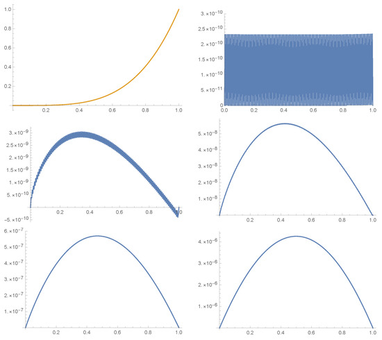
Figure 4.
The analytical solution y and the numerical solutions for different value of (left top panel). The approximation error for (right top panel), (left middle panel), (right middle panel), (left bottom panel), (right bottom panel).
5. Conclusions
We have presented a collocation method based on the Schoenberg-Bernstein quasi-interpolant operator and used the method to efficiently solve boundary value problems having Caputo fractional derivative. The numerical results shown in Section 4 show that the method is accurate and exact on linear functions. We notice that we can increase the approximation order using different kind of quasi-interpolant operators, like the discrete operators introduced in References [32,35]. Some first results in this direction can be found in Reference [47]. Finally, we notice that even if the B-spline basis is centrally symmetric in the interval , its Caputo fractional derivative is not. The symmetry could be recovered replacing the Caputo derivative with the Riesz derivative defined as [4]
which is centrally symmetric in the interval . The solution of boundary value problems having Riesz fractional derivative in space will be the subject of a forthcoming paper.
Funding
This research was partially funded by Gruppo Nazionale per il Calcolo Scientifico (Istituto Nazionale di Alta Matematica ‘Francesco Severi’), grant INdAM–GNCS Project 2020 “Costruzione di metodi numerico/statistici basati su tecniche multiscala per il trattamento di segnali e immagini ad alta dmensionalità”.
Conflicts of Interest
The authors declare no conflict of interest.
References
- Hilfer, R. Applications of Fractional Calculus in Physics; World Scientific: Singapore, 2000. [Google Scholar]
- Kilbas, A.A.; Srivastava, H.M.; Trujillo, J.J. Theory and Applications of Fractional Differential Equations; Elsevier Science: Amsterdam, The Netherlands, 2006. [Google Scholar]
- Mainardi, F. Fractional Calculus and Waves in Linear Viscoelasticity: An Introduction to Mathematical Models; World Scientific: Singapore, 2010. [Google Scholar]
- Samko, S.G.; Kilbas, A.A.; Marichev, O.I. Fractional Integrals and Derivatives; Gordon & Breach Science Publishers: Switzerland, 1993. [Google Scholar]
- Tarasov, V.E. Fractional Dynamics; Nonlinear Physical Science; Springer: Berlin/Heidelberg, Germany, 2010. [Google Scholar] [CrossRef]
- Diethelm, K. The Analysis of Fractional Differential Equations: An Application-Oriented Exposition Using Differential Operators of Caputo Type; Springer: Berlin/Heidelberg, Germany, 2010. [Google Scholar]
- Diethelm, K.; Freed, A.D. On the solution of nonlinear fractional-order differential equations used in the modeling of viscoplasticity. In Scientific Computing in Chemical Engineering II; Springer: Berlin/Heidelberg, Germany, 1999; pp. 217–224. [Google Scholar]
- Mainardi, F.; Luchko, Y.; Pagnini, G. The fundamental solution of the space-time fractional diffusion equation. Fract. Calc. Appl. Anal. 2007, 4, 153–192. [Google Scholar]
- Agarwal, R.P.; Benchohra, M.; Hamani, S. A survey on existence results for boundary value problems of nonlinear fractional differential equations and inclusions. Acta Appl. Math. 2010, 109, 973–1033. [Google Scholar] [CrossRef]
- Pedas, A.; Tamme, E. Piecewise polynomial collocation for linear boundary value problems of fractional differential equations. J. Comput. Appl. Math. 2012, 236, 3349–3359. [Google Scholar] [CrossRef]
- Acosta, G.; Borthagaray, J.P.; Bruno, O.; Maas, M. Regularity theory and high order numerical methods for the (1D)-fractional Laplacian. Math. Comput. 2018, 87, 1821–1857. [Google Scholar] [CrossRef]
- Oldham, K.; Spanier, J. The Fractional Calculus; Academic Press: Cambridge, MA, USA, 1974. [Google Scholar]
- Podlubny, I. Fractional Differential Equations; Academic Press: Cambridge, MA, USA, 1998. [Google Scholar]
- He, J.H. A tutorial review on fractal spacetime and fractional calculus. Int. J. Theor. Phys. 2014, 53, 3698–3718. [Google Scholar] [CrossRef]
- Caputo, M.; Fabrizio, M. A new definition of fractional derivative without singular kernel. Progr. Fract. Differ. Appl 2015, 1, 1–13. [Google Scholar]
- He, J.H. Homotopy perturbation technique. Comput. Methods Appl. Mech. Eng. 1999, 178, 257–262. [Google Scholar] [CrossRef]
- He, J.H.; Wu, G.C.; Austin, F. The variational iteration method which should be followed. Nonlinear Sci. Lett. A 2010, 1, 1–30. [Google Scholar]
- Liu, H.Y.; He, J.H.; Li, Z.B. Fractional calculus for nanoscale flow and heat transfer. Int. J. Numer. Methods Heat Fluid Flow 2014, 24, 1227–1250. [Google Scholar] [CrossRef]
- Momani, S.; Odibat, Z. Comparison between the homotopy perturbation method and the variational iteration method for linear fractional partial differential equations. Comput. Math. Appl. 2007, 54, 910–919. [Google Scholar] [CrossRef]
- Odibat, Z.; Momani, S. The variational iteration method: An efficient scheme for handling fractional partial differential equations in fluid mechanics. Comput. Math. Appl. 2009, 58, 2199–2208. [Google Scholar] [CrossRef]
- Ervin, V.J.; Roop, J.P. Variational formulation for the stationary fractional advection dispersion equation. Numer. Methods Partial Differ. Equ. Int. J. 2006, 22, 558–576. [Google Scholar] [CrossRef]
- Ford, N.J.; Morgado, M. Fractional boundary value problems: Analysis and numerical methods. Fract. Calc. Appl. Anal. 2011, 14, 554–567. [Google Scholar] [CrossRef]
- Chen, S.; Shen, J.; Wang, L.L. Generalized Jacobi functions and their applications to fractional differential equations. Math. Comput. 2016, 85, 1603–1638. [Google Scholar] [CrossRef]
- Mao, Z.; Karniadakis, G.E. A spectral method (of exponential convergence) for singular solutions of the diffusion equation with general two-sided fractional derivative. SIAM J. Numer. Anal. 2018, 56, 24–49. [Google Scholar] [CrossRef]
- Ismail, M.; Saeed, U.; Alzabut, J.; Rehman, M. Approximate solutions for fractional boundary value problems via green-cas wavelet method. Mathematics 2019, 7, 1164. [Google Scholar] [CrossRef]
- Baleanu, D.; Diethelm, K.; Scalas, E.; Trujillo, J.J. Fractional Calculus: Models and Numerical Methods; World Scientific: Singapore, 2016. [Google Scholar]
- Li, C.; Zeng, F. Numerical Methods for Fractional Calculus; CRC Press: Boca Raton, FL, USA, 2015; Volume 24. [Google Scholar]
- Pitolli, F. A fractional B-spline collocation method for the numerical solution of fractional predator-prey models. Fractal Fract. 2018, 2, 13. [Google Scholar] [CrossRef]
- Cai, M.; Li, C. Numerical approaches to fractional integrals and derivatives: A review. Mathematics 2020, 8, 43. [Google Scholar] [CrossRef]
- Diethelm, K.; Garrappa, R.; Stynes, M. Good (and not so good) practices in computational methods for fractional calculus. Mathematics 2020, 8, 324. [Google Scholar] [CrossRef]
- De Boor, C.; Fix, G.J. Spline approximation by quasiinterpolants. J. Approx. Theory 1973, 8, 19–45. [Google Scholar] [CrossRef]
- Lyche, T.; Schumaker, L.L. Local spline approximation methods. J. Approx. Theory 1975, 15, 294–325. [Google Scholar] [CrossRef]
- Goodman, T.N.T.; Sharma, A. A Modified Bernstein-Schoenberg Operator. In Constructive Theory of Functions 87; Sendov, B., Ed.; Bulgarian Academy Sciences: Sofia, Bulgaria, 1988. [Google Scholar]
- Lee, B.G.; Lyche, T.; Mørken, K. Some examples of quasi-interpolants constructed from local spline projectors. In Mathematical Methods for Curves and Surfaces. Oslo 2000; Lyche, T., Schumaker, L., Eds.; Vanderbilt University Press: Nashville, TN, USA, 2001; pp. 243–252. [Google Scholar]
- Sablonnière, P. Recent progress on univariate and multivariate polynomial and spline quasi-interpolants. In Trends and Applications in Constructive Approximation; De Bruin, M., Mache, D., Szabados, J., Eds.; Birkhäuser Verlag: Basel, Switzerland, 2005; Volume 177, pp. 229–245. [Google Scholar]
- Schoenberg, I.J. On spline functions. In Inequalities; Shisha, O., Ed.; Academic Press: New York, NY, USA, 1967; pp. 255–291. [Google Scholar]
- Pezza, L.; Pitolli, F. A multiscale collocation method for fractional differential problems. Math. Comput. Simul. 2018, 147, 210–219. [Google Scholar] [CrossRef]
- Pellegrino, E.; Pezza, L.; Pitolli, F. A collocation method in spline spaces for the solution of linear fractional dynamical systems. Math. Comput. Simul. 2019, 176, 266–278. [Google Scholar] [CrossRef]
- Kolk, M.; Pedas, A.; Tamme, E. Smoothing transformation and spline collocation for linear fractional boundary value problems. Appl. Math. Comput. 2016, 283, 234–250. [Google Scholar] [CrossRef]
- Vainikko, G. Multidimensional Weakly Singular Integral Equations; Lecture Notes in Mathematics; Springer: Berlin/Heidelberg, Germany, 1993; Volume 1549. [Google Scholar]
- De Boor, C. A Practical Guide to Splines; Springer: Berlin/Heidelberg, Germany, 1978. [Google Scholar]
- Schumaker, L.L. Spline Functions: Basic Theory; Cambridge University Press: Cambridge, UK, 2007. [Google Scholar]
- Pitolli, F. Optimal B-spline bases for the numerical solution of fractional differential problems. Axioms 2018, 7, 46. [Google Scholar] [CrossRef]
- Unser, M.; Blu, T. Fractional splines and wavelets. SIAM Rev. 2000, 42, 43–67. [Google Scholar] [CrossRef]
- Marsden, M.J. An identity for spline functions with applications to variation diminishing spline approximation. J. Approx. Theory 1970, 3, 7–49. [Google Scholar] [CrossRef]
- Ascher, U. Discrete least squares approximations for ordinary differential equations. SIAM J. Numer. Anal. 1978, 15, 478–496. [Google Scholar] [CrossRef]
- Pellegrino, E.; Pezza, L.; Pitolli, F. A collocation method based on discrete quasi-interpolatory operators for the solution of time fractional differential problems. 2020; in preparation. [Google Scholar]


© 2020 by the author. Licensee MDPI, Basel, Switzerland. This article is an open access article distributed under the terms and conditions of the Creative Commons Attribution (CC BY) license (http://creativecommons.org/licenses/by/4.0/).