Dynamics of HIV-TB Co-Infection Model

Abstract

According to World Health Organization (WHO), the population suffering from human immunodeficiency virus (HIV) infection over a period of time may suffer from TB infection which increases the death rate. There is no cure for acquired immunodeficiency syndrome (AIDS) to date but antiretrovirals (ARVs) can slow down the progression of disease as well as prevent secondary infections or complications. This is considered as a medication in this paper. This scenario of HIV-TB co-infection is modeled using a system of non-linear differential equations. This model considers HIV-infected individual as the initial stage. Four equilibrium points are found. Reproduction number R₀ is calculated. If R₀ >1 disease persists uniformly, with reference to the reproduction number, backward bifurcation is computed for pre-AIDS (latent) stage. Global stability is established for the equilibrium points where there is no Pre-AIDS TB class, point without co-infection and for the endemic point. Numerical simulation is carried out to validate the data. Sensitivity analysis is carried out to determine the importance of model parameters in the disease dynamics.

1. Introduction

In the public health sector, human immunodeficiency virus (HIV) continues to be the major health threat globally, having claimed more than 32 million lives to date [1]. There were approximately 37.9 million people living with HIV at the end of 2018 [1]. The human immunodeficiency virus (HIV) is a virus that spread through certain body fluids, attacking the body′s immune system, specifically the CD4 cells. The immune function is typically measured by CD4 cell count. Over time, HIV can destroy so many of these cells that the body can’t fight against infections and diseases, which paves the way for many opportunistic diseases. One such disease is tuberculosis (TB). It is a contagious disease caused by bacteria called Mycobacterium tuberculosis. The bacteria mostly attack the lungs, but can also damage other parts of the body. The population living with HIV are 15–22 times more likely to develop TB [2]. It is the most commonly occurring illness among HIV-infected individuals, including among those taking antiretroviral treatment (ART). This interaction explains the fact that HIV and TB co-infection is a deadly human syndemic, where syndemic refers to the convergence of two or more diseases that exacerbate the burden of the disease [3]. For the treatment of HIV, HIV drugs called antiretrovirals (ARVs) are advised. ART reduces the risk of TB infection in people living with HIV by 65% [4]. It plays a significant role in preventing TB.

Mathematical modelling has enhanced understanding of disease dynamics. The first compartmental model was given by Kermack and McKendrick [5]. Some basic papers like [6,7] have constructed mathematical models by formulating non-linear differential equation for their respective models and have worked out the critical point/equilibrium points of the respective system and various related properties. In some the related research, many authors have worked out various types of HIV-TB co-infection model. Kirschner et al. [8] developed a model for HIV-1 and TB coinfection inside a host. This was the first attempt to understand how TB affects the dynamics of HIV-infected individuals. TB is known to be the common serious opportunistic infection occurring in HIV individuals and it occurs in more than 50% of the acquired immunodeficiency syndrome (AIDS) cases in developing countries. Naresh et al. [9] developed a simple nonlinear mathematical model dividing the population into four sub-classes, namely the susceptible, TB-infective, HIV-infective and AIDS patients. The treatment class in the HIV-AIDS co-infection model was first introduced by Huo et al. [10], however, Bhunu et al. [11] in his co-infection model considered all aspects of TB and HIV transmission dynamics with both HIV and TB treatment. This paper incorporated ARTs for AIDS cases and studied its implication on TB. However, the author did not consider the case where individual co-infected with HIV-TB can effectively recover from TB infection. Another HIV-TB co-infection model was formulated by Roeger et al. [12], assuming TB-infected individuals in the active stage of disease to be sexually inactive. Singh et al. [13] studied the transmission dynamics of the HIV/AIDS epidemic model considering three different latent stages based on treatment. Torres et al. [14], in his model, incorporates both TB and AIDS treatment for individuals suffering with either or both disease.

The model formulated in this paper considers the susceptible class to be HIV-infected. The paper is organized as follows. The model is formulated and its description is given in Section 2. Calculation of reproduction number and uniform persistence of the disease is shown in Section 2.3. In Section 2.4, global stability for all the equilibrium points is done. In Section 3, backward bifurcation is established. The sensitivity of reproduction number is done in Section 3.1. Section 3.2 presents a numerical simulation. The paper concludes in Section 4.

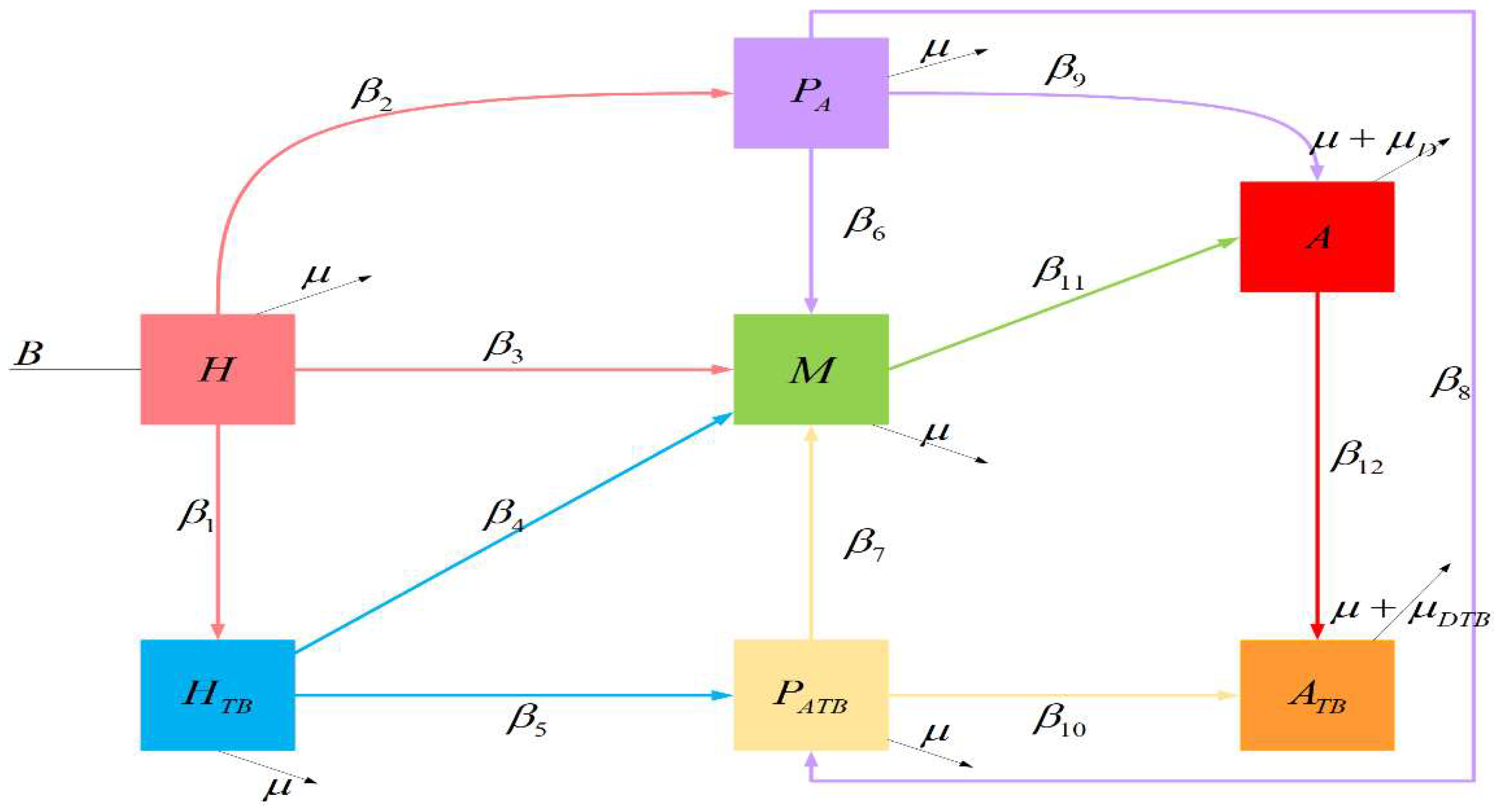
2. Mathematical Model

We begin with seven mutually exclusive compartmental models showing HIV-TB co-infection. In this model, the human population is divided into sub-populations as follows: acute HIV-infected individuals ($H$), co-infected with HIV-TB ($H_{TB}$), Pre-AIDS stage($P_A$), infected individuals undergoing any type of treatment say ARV’s and any TB treatment ($M$), Pre-AIDS stage with TB disease ($P_{ATB}$), HIV-infected individuals showing clinical AIDS symptoms ($A$), HIV-infected individuals with AIDS symptoms coinfected with TB disease ($A_{TB}$).

The notations and parametric values assumed in the paper for the study of dynamical system of HIV-TB co-infection model is tabulated in

Table 1. Parametric definitions and its values.

Notations	Description	Parametric Values
$N(t)$	Number of individuals at any instant of time	100
$B$	Birth rate	0.2
${\beta }_1$	Rate at which co-infection occurs	0.45
${\beta }_2$	Rate at which HIV-infected individuals reaches pre-AIDS stage	0.48
${\beta }_3$	Rate at which HIV-infected individualsopt for medication	0.31
${\beta }_4$	Rate at which co-infected individual goes for medication	0.1
${\beta }_5$	Rate at which co-infection (HIV-TB) individual joins pre-AIDS TB stage	0.037
${\beta }_6$	Rate at which pre-AIDS infectives opt for medication	0.25
${\beta }_7$	Rate at which pre-AIDS TB infectives undergo medication	0.15
${\beta }_8$	Rate at which pre-AIDS infected individuals join pre-AIDS TB class	0.8
${\beta }_9$	Rate at which pre-AIDS suffer from full-blown AIDS	0.3
${\beta }_{10}$	Rate at which Pre-AIDS TB infectives joins full-blown AIDS TB class	0.001
${\beta }_{11}$	Rate at which treated infectives move to AIDS class	0.78
${\beta }_{12}$	Rate at which individuals with full-blown AIDS suffer from TB	0.35
$\mu$	Natural death rate	0.002
${\mu }_D$	Death rate due to AIDS	0.6
${\mu }_{DTB}$	Death rate due to co-infection	0.52

.

In this paper, the susceptible class is considered to be HIV-infected (acute HIV infection). This class is increased by recruitments of newly HIV-infected individuals at the rate $B$. All the individuals in their respective compartments suffer from natural death at the constant rate $\mu$. Individuals undergoing medication (treatment) through ARTs lower the rate of progression from HIV disease to AIDS, as HIV can never be cured.

Here, the individuals infected with HIV develop a very weak immune system, which means they are likely to get infected by many opportunistic diseases. As TB is considered to be one of the most commonly occurring disease among HIV patients [15], the individual infected with HIV gets TB disease moving towards $H_{TB}$ by rate ${\beta }_1$. The HIV-infected individuals are also assumed to progress to the asymptotic pre-AIDS class ($P_A$) at the rate ${\beta }_2$. The HIV-infected and co-infected individuals undergoing treatment move to class $M$ with the rates ${\beta }_3$ and ${\beta }_4$, respectively. Similarly, individuals with a co-infection of HIV-TB move towards $P_{ATB}$ with the rate ${\beta }_5$. Individuals showing symptoms of AIDS ($P_A$) suffer from full-blown AIDS, joining $A$, at the rate ${\beta }_9$, and they are more likely to develop TB, progressing to class $P_{ATB}$ with the rate ${\beta }_8$. $P_A$ class individuals undergoing ARTs treatment (anti-retroviral therapy) join $M$ at the rate ${\beta }_6$. Individuals in $P_{ATB}$ are treated for TB at the constant rate ${\beta }_7$, joining $M$, and some of them can also develop full-blown AIDS, moving to $A_{TB}$ class with the constant rate ${\beta }_{10}$. Treated individuals, recovered from TB but still with HIV infection (as it cannot be cured) move to full-blown AIDS ($A$) with the constant rate ${\beta }_{11}$. Individuals suffering with AIDS have such a badly damaged immune system that they get an increasing number of severe illnesses (here, TB) and hence move towards full-blown AIDS-TB class with the constant rate ${\beta }_{12}$. The death rates ${\mu }_D$ and ${\mu }_{DTB}$ are considered as deaths due to individuals infected with AIDS and AIDS-TB, respectively.

2.1. HIV-TB Co-infection Model

Considering the aforementioned assumptions and Figure 1 gives rise to the following set of non-linear differential equations for the HIV-TB co-infection model:

$$\begin{array}{l}\frac{dH}{dt}=B-{\beta }_{1}H{H}_{TB}-({\beta }_2+{\beta }_3+\mu )H\\ \frac{d{H}_{TB}}{dt}={\beta }_{1}H{H}_{TB}-{\beta }_5{H}_{TB}{P}_{ATB}-(\mu +{\beta }_4)H_{TB}\\ \frac{d{P}_A}{dt}={\beta }_{2}H-{\beta }_8{P}_A{P}_{ATB}-(\mu +{\beta }_6+{\beta }_9)P_A\\ \frac{dM}{dt}={\beta }_{3}H+{\beta }_4{H}_{TB}+{\beta }_6{P}_A+{\beta }_7{P}_{ATB}-(\mu +{\beta }_{11})M\\ \frac{d{P}_{ATB}}{dt}={\beta }_5{H}_{TB}{P}_{ATB}+{\beta }_8{P}_A{P}_{ATB}-(\mu +{\beta }_7+{\beta }_{10})P_{ATB}\\ \frac{dA}{dt}={\beta }_9{P}_A+{\beta }_{11}M-(\mu +{\mu }_D+{\beta }_{12})A\\ \frac{d{A}_{TB}}{dt}={\beta }_{10}{P}_{ATB}+{\beta }_{12}A-(\mu +{\mu }_{DTB})A_{TB}\end{array}$$

(1)

where $N(t)=H(t)+H_{TB}(t)+P_A(t)+M(t)+P_{ATB}(t)+A(t)+A_{TB}(t)$.

The system satisfies the conditions:

$$H(t)\ge 0,H_{TB}(t)\ge 0,P_A(t)\ge 0,M(t)\ge 0,P_{ATB}(t)\ge 0,A(t)\ge 0,A_{TB}(t)\ge 0$$

Adding the above set of differential equations, we get,

$$\begin{array}{l}\frac{dN(t)}{dt}=B-\mu (H+H_{TB}+P_A+M+P_{ATB}+A+A_{TB})-{\mu }_{D}A-{\mu }_{DTB}{A}_{TB}\\ \le B-\mu (H+H_{TB}+P_A+M+P_{ATB}+A+A_{TB})\end{array}$$

Hence, $\frac{dN(t)}{dt}\le B-\mu N$, so that $\underset{t\to \infty }{\lim }\sup N\le \frac{B}{\mu }$

The feasible region for the system is defined as

$$\Lambda =\left\{(H,H_{TB},P_A,M,P_{ATB},A,A_{TB}):0\le H+H_{TB}+P_A+M+P_{ATB}+A+A_{TB}\le \frac{B}{\mu }\right\}$$

We assume $L_1={\beta }_2+{\beta }_3,\hspace{1em}{L}_2={\beta }_6+{\beta }_9,\hspace{1em}{L}_3={\beta }_7+{\beta }_{10}$. The modified system is

$$\begin{array}{l}\frac{dH}{dt}=B-{\beta }_{1}H{H}_{TB}-(L_1+\mu )H\\ \frac{d{H}_{TB}}{dt}={\beta }_{1}H{H}_{TB}-{\beta }_5{H}_{TB}{P}_{ATB}-(\mu +{\beta }_4)H_{TB}\\ \frac{d{P}_A}{dt}={\beta }_{2}H-{\beta }_8{P}_A{P}_{ATB}-(L_2+\mu )P_A\\ \frac{dM}{dt}={\beta }_{3}H+{\beta }_4{H}_{TB}+{\beta }_6{P}_A+{\beta }_7{P}_{ATB}-(\mu +{\beta }_{11})M\\ \frac{d{P}_{ATB}}{dt}={\beta }_5{H}_{TB}{P}_{ATB}+{\beta }_8{P}_A{P}_{ATB}-(L_3+\mu )P_{ATB}\\ \frac{dA}{dt}={\beta }_9{P}_A+{\beta }_{11}M-(\mu +{\mu }_D+{\beta }_{12})A\\ \frac{d{A}_{TB}}{dt}={\beta }_{10}{P}_{ATB}+{\beta }_{12}A-(\mu +{\mu }_{DTB})A_{TB}\end{array}$$

(2)

System (1) and (2) are equivalent, hence $\Lambda$ is also the feasible region for system (2).

2.2. Equilibrium Solutions

Equating $\frac{dH}{dt}=\frac{d{H}_{TB}}{dt}=\frac{d{P}_A}{dt}=\frac{dM}{dt}=\frac{d{P}_{ATB}}{dt}=\frac{dA}{dt}=\frac{d{A}_{TB}}{dt}=0$ and solving for the compartments following are the equilibria:

• $E_1(H_1,0,P_{A_1},M_1,0,A_1,A_{T{B}_1})$

  $$\begin{array}{c}{H}_1=\frac{B}{L_1+\mu },H_{T{B}_1}=0,P_{A_1}=\frac{B{\beta }_2}{(L_1+\mu )(L_2+\mu )},M_1=\frac{B(L_2{\beta }_3+{\beta }_2{\beta }_6+{\beta }_3\mu )}{(L_1+\mu )(L_2+\mu )({\beta }_{11}+\mu )},\\ P_{AT{B}_1}=0,A_1=\frac{B({\beta }_{11}(L_2{\beta }_3+{\beta }_2{\beta }_6+{\beta }_3\mu )+{\beta }_2{\beta }_9({\beta }_{11}+\mu ))}{(L_1+\mu )(L_2+\mu )({\beta }_{11}+\mu )(\mu +{\mu }_D+{\beta }_{12})},\\ A_{T{B}_1}=\frac{B{\beta }_{12}({\beta }_{11}(L_2{\beta }_3+{\beta }_2{\beta }_6+{\beta }_3\mu )+{\beta }_2{\beta }_9({\beta }_{11}+\mu ))}{(L_1+\mu )(L_2+\mu )({\beta }_{11}+\mu )(\mu +{\mu }_D+{\beta }_{12})(\mu +{\mu }_D)}.\end{array}$$
• $E_2(H_2,0,P_{A_2},M_2,P_{AT{B}_2},A_2,A_{T{B}_2})$

  $$\begin{array}{l}{H}_2=\frac{B}{L_1+\mu },H_{T{B}_2}=0,P_{A_2}=\frac{L_3+\mu }{{\beta }_8},P_{AT{B}_2}=\frac{B{\beta }_2{\beta }_8-(L_1+\mu )(L_2+\mu )(L_3+\mu )}{{\beta }_8(L_1+\mu )(L_3+\mu )},\\ M_2=\frac{B{\beta }_8(L_3{\beta }_3+{\beta }_2{\beta }_7+{\beta }_3\mu )+(L_1+\mu )(L_3+\mu )({\beta }_6(L_3+\mu )-{\beta }_7(L_2+\mu ))}{{\beta }_8(L_1+\mu )(L_3+\mu )({\beta }_{11}+\mu )},\\ A_2=\frac{\begin{array}{l}\{B{\beta }_8{\beta }_{11}(L_3{\beta }_3+{\beta }_2{\beta }_7+{\beta }_3\mu )+{(L_3+\mu )}^2(L_1+\mu )\\ ({\beta }_9({\beta }_{11}+\mu )+{\beta }_6{\beta }_{11})-(L_1+\mu )(L_2+\mu )(L_3+\mu ){\beta }_7{\beta }_{11}\}\end{array}}{{\beta }_8(L_1+\mu )(L_3+\mu )(\mu +{\mu }_D+{\beta }_{12})},\\ A_{T{B}_2}=\frac{\begin{array}{l}B{\beta }_8{\beta }_{11}{\beta }_{12}({\beta }_2{\beta }_7+L_3{\beta }_3+\mu {\beta }_3)+({\beta }_{11}+\mu ){\mu }_{D}B{\beta }_2{\beta }_8{\beta }_{10}-(L_1+\mu )(L_2+\mu )\\ (L_3+\mu )({\beta }_7{\beta }_{11}{\beta }_{12}+({\beta }_{11}+\mu ){\mu }_D{\beta }_{10})+({\beta }_{12}+\mu )({\beta }_{11}+\mu )B{\beta }_2{\beta }_8{\beta }_{10}+(L_1+\mu )\\ (L_3+\mu )({\beta }_6{\beta }_{11}+({\beta }_{11}+\mu ){\beta }_9{\beta }_{12})-(L_1+\mu )(L_2+\mu )(L_3+\mu )({\beta }_{11}+\mu )({\beta }_{12}+\mu )\end{array}}{{\beta }_8(L_1+\mu )(L_3+\mu )({\beta }_{11}+\mu )(\mu +{\mu }_{DTB})(\mu +{\mu }_D+{\beta }_{12})}\end{array}$$
• $E_3(H_3,H_{T{B}_3},P_{A_3},M_3,0,A_3,A_{T{B}_3})$

  $$\begin{array}{l}{H}_3=\frac{{\beta }_4+\mu }{{\beta }_1},H_{T{B}_3}=\frac{B{\beta }_1-(L_1+\mu )({\beta }_4+\mu )}{{\beta }_1({\beta }_4+\mu )},P_{A_3}=\frac{{\beta }_2({\beta }_4+\mu )}{{\beta }_1(L_2+\mu )},\\ M_3=\frac{(L_2+\mu )(B{\beta }_1{\beta }_4-({\beta }_4+\mu )(L_1{\beta }_4-{\beta }_3{\beta }_4-{\beta }_3\mu -{\beta }_4\mu ))+{\beta }_2{\beta }_6{({\beta }_4+\mu )}^2}{{\beta }_1(L_2+\mu )({\beta }_4+\mu )({\beta }_{11+\mu })},\\ P_{AT{B}_3}=0,A_3=\frac{\begin{array}{l}\{{\beta }_4{\beta }_{11}(B{\beta }_1-L_1({\beta }_4+\mu ))(L_2+\mu )+({\beta }_4+\mu )(L_2{\beta }_{11}({\beta }_3{\beta }_4+{\beta }_3\mu -{\beta }_4\mu )\\ -{\beta }_4{\beta }_{11}{\mu }^2)+{({\beta }_4+\mu )}^2({\beta }_2{\beta }_9({\beta }_{11}+\mu )+{\beta }_2{\beta }_6{\beta }_{11}+{\beta }_3{\beta }_{11}\mu )\}\end{array}}{{\beta }_1(L_2+\mu )({\beta }_4+\mu )({\beta }_{11}+\mu )(\mu +{\mu }_D+{\beta }_{12})}\\ A_{T{B}_3}=\frac{\begin{array}{l}\{{\beta }_{12}({\beta }_4{\beta }_{11}(B{\beta }_1-L_1({\beta }_4+\mu ))(L_2+\mu )+({\beta }_4+\mu )(L_2{\beta }_{11}({\beta }_3{\beta }_4+{\beta }_3\mu -{\beta }_4\mu )\\ -{\beta }_4{\beta }_{11}{\mu }^2))+{({\beta }_4+\mu )}^2({\beta }_2{\beta }_9({\beta }_{11}+\mu )+{\beta }_2{\beta }_6{\beta }_{11}+{\beta }_3{\beta }_{11}\mu )\}\end{array}}{{\beta }_1(L_2+\mu )({\beta }_4+\mu )({\beta }_{11}+\mu )(\mu +{\mu }_D+{\beta }_{12})(\mu +{\mu }_{DTB})}\end{array}$$
• Endemic Equilibrium point $E^{*}(H^{*},H_{TB}^{*},P_A^{*},M^{*},P_{ATB}^{*},A^{*},A_{TB}^{*})$

  $$\begin{array}{c}{H}^{*}=\frac{r({\beta }_8({\beta }_4+\mu )-{\beta }_5(L_2+\mu ))+B{\beta }_5}{{\beta }_5(L_1+\mu )+{\beta }_1(L_3+\mu )-{\beta }_2{\beta }_5},H_{TB}^{*}=\frac{-{\beta }_{8}r+L_3+\mu }{{\beta }_5},P_A^{*}=r,\\ P_{ATB}^{*}=\frac{\begin{array}{l}r{\beta }_1({\beta }_8({\beta }_4+\mu )-{\beta }_5(L_2+\mu ))+{\beta }_5(B{\beta }_1\\ -(L_1+\mu )({\beta }_4+\mu )+{\beta }_2({\beta }_4+\mu ))-{\beta }_1(L_3+\mu )({\beta }_4+\mu )\end{array}}{{\beta }_5(L_1{\beta }_5+L_3{\beta }_1+{\beta }_1\mu -{\beta }_2{\beta }_5+{\beta }_5\mu )},\end{array}$$

  $$\begin{array}{l}{M}^{*}=\frac{\begin{array}{l}r[({\beta }_5{\beta }_6-{\beta }_4{\beta }_8)[{\beta }_5(L_1+\mu )+{\beta }_1(L_3+\mu )-{\beta }_2{\beta }_5]+({\beta }_3{\beta }_5+{\beta }_7{\beta }_{11})({\beta }_8({\beta }_4+\mu )\\ -{\beta }_5(L_2+\mu ))]+{\beta }_5{\beta }_7[(B{\beta }_1-(L_1+\mu )({\beta }_4+\mu ))+{\beta }_2({\beta }_4+\mu )]+{\beta }_4{\beta }_5(L_1+\mu )\\ (L_3+\mu )+(L_3+\mu ){\beta }_1({\beta }_4(L_3+\mu )-{\beta }_7({\beta }_4+\mu ))-{\beta }_2{\beta }_4{\beta }_5(L_3+\mu )+B{\beta }_3{\beta }_5^2\end{array}}{{\beta }_5({\beta }_{11}+\mu )({\beta }_5(L_1+\mu )+{\beta }_1(L_3+\mu )-{\beta }_2{\beta }_5)},\\ A^{*}=\frac{\begin{array}{l}r({\beta }_{11}({\beta }_1{\beta }_7+{\beta }_3{\beta }_5)({\beta }_8({\beta }_4+\mu )-{\beta }_5(L_2+\mu ))+({\beta }_1(L_3+\mu )+{\beta }_5(L_1+\mu )-{\beta }_2{\beta }_5)\\ (({\beta }_{11}+\mu ){\beta }_5{\beta }_9+({\beta }_5{\beta }_6-{\beta }_4{\beta }_8){\beta }_{11}))+{\beta }_{11}({\beta }_5{\beta }_7(B{\beta }_1-(L_1+\mu )({\beta }_4+\mu ))+{\beta }_2({\beta }_4+\mu ))\\ +{\beta }_4{\beta }_5(L_1+\mu )(L_3+\mu )+{\beta }_1(L_3+\mu )({\beta }_4(L_3+\mu )-{\beta }_7({\beta }_4+\mu ))-{\beta }_2{\beta }_4{\beta }_5(L_3+\mu )+B{\beta }_3{\beta }_5^2\end{array}}{{\beta }_5(\mu +{\beta }_{11})(\mu +{\mu }_D+{\beta }_{12})({\beta }_5(L_1+\mu )+{\beta }_1(L_3+\mu )-{\beta }_2{\beta }_5)},\\ A_{TB}^{*}=\frac{\begin{array}{l}r[({\beta }_8({\beta }_4+\mu )-{\beta }_5(L_2+\mu ))(({\beta }_{11}+\mu ){\beta }_1{\beta }_{10}(\mu +{\mu }_D+{\beta }_{12})+{\beta }_{11}{\beta }_{12}({\beta }_3{\beta }_5+{\beta }_1{\beta }_7))\\ +({\beta }_5(L_1+\mu )+{\beta }_1(L_3+\mu )-{\beta }_2{\beta }_5){\beta }_{12}(({\beta }_4+\mu ){\beta }_5{\beta }_9+({\beta }_5{\beta }_6-{\beta }_4{\beta }_8){\beta }_{11})]+{\mu }_D{\beta }_{10}\\ ({\beta }_{11}+\mu )({\beta }_4+\mu )({\beta }_2{\beta }_5-{\beta }_1(L_3+\mu )-{\beta }_5(L_1+\mu ))+{\mu }_{D}B{\beta }_1{\beta }_5{\beta }_{10}({\beta }_{11}+\mu )+{\beta }_7{\beta }_{11}{\beta }_{12}\\ ({\beta }_4+\mu )({\beta }_2{\beta }_5-{\beta }_5\mu -L_3{\beta }_1)-{\beta }_{10}({\beta }_{12}+\mu ){({\beta }_{11}+\mu )}^2({\beta }_5(L_1+\mu )+{\beta }_1(L_3+\mu ))+{\beta }_4\\ {\beta }_{11}{\beta }_{12}(L_3+\mu )({\beta }_5(L_1+\mu )+{\beta }_1(L_3+\mu )-{\beta }_2{\beta }_5)+{\beta }_5{\beta }_{10}({\beta }_{11}+\mu )({\beta }_{12}+\mu )({\beta }_2({\beta }_4+\mu )\\ +B{\beta }_1)-{\beta }_1{\beta }_7{\beta }_{11}{\beta }_{12}({\beta }_5+\mu )({\beta }_4+\mu )+B{\beta }_5{\beta }_{11}{\beta }_{12}({\beta }_1{\beta }_7+{\beta }_3{\beta }_5)\end{array}}{{\beta }_5(\mu +{\beta }_{11})(\mu +{\mu }_{DTB})(\mu +{\mu }_D+{\beta }_{12})({\beta }_5(L_1+\mu )+{\beta }_1(L_3+\mu )-{\beta }_2{\beta }_5)}\end{array}$$

  where, $\begin{array}{l}r=rootof(({\beta }_1{\beta }_8({\beta }_5(L_2+\mu )-{\beta }_8({\beta }_4+\mu )))Z^2+(-{\beta }_5{\beta }_8(B{\beta }_1-(L_1+\mu )({\beta }_4+\mu ))\\ \hspace{1em}-{\beta }_5^2(L_1+\mu )(L_2+\mu )+{\beta }_1(L_3+\mu )({\beta }_8({\beta }_4+\mu )-{\beta }_5(L_2+\mu )))Z+B{\beta }_2{\beta }_5^2\end{array}$.

2.3. Reproduction Number

The reproduction number measures the expected number of secondary infected individuals produced due to an infected individual during the entire death period in an uninfected population.

In this paper, reproduction number R₀ is defined as the number of infected individuals due to an AIDS- or TB-infected individual in the HIV infected-population. It is calculated using next-generation matrix method [16] and is defined as the spectral radius of $F{V}^{-1}$ at $E_1$.

where, $F=\left[\begin{array}{ccccccc}{\beta }_{1}H& 0& 0& 0& 0& 0& {\beta }_1{H}_{TB}\\ 0& 0& 0& 0& 0& 0& 0\\ 0& 0& 0& 0& 0& 0& 0\\ {\beta }_5{P}_{ATB}& {\beta }_8{P}_{ATB}& 0& {\beta }_5{H}_{TB}+{\beta }_8{P}_A& 0& 0& 0\\ 0& 0& 0& 0& 0& 0& 0\\ 0& 0& 0& 0& 0& 0& 0\\ 0& 0& 0& 0& 0& 0& 0\end{array}\right]$

$$V=\left[\begin{array}{ccccccc}{\beta }_4+{\beta }_5{P}_{ATB}+\mu & 0& 0& {\beta }_5{H}_{TB}& 0& 0& 0\\ 0& {\beta }_8{P}_{ATB}+L_2+\mu & 0& {\beta }_8{P}_A& 0& 0& -{\beta }_2\\ -{\beta }_4& -{\beta }_6& {\beta }_{11}+\mu & -{\beta }_7& 0& 0& -{\beta }_3\\ 0& 0& 0& L_3+\mu & 0& 0& 0\\ 0& -{\beta }_9& -{\beta }_{11}& 0& {\beta }_{12}+{\mu }_D+\mu & 0& 0\\ 0& 0& 0& -{\beta }_{10}& -{\beta }_{12}& \mu +{\mu }_{DTB}& 0\\ {\beta }_{1}H& 0& 0& 0& 0& 0& {\beta }_1{H}_{TB}+L_1+\mu \end{array}\right]$$

The dominant eigenvalue of $F{V}^{-1}$ at $E_1$ is $R_0=\frac{B{\beta }_2{\beta }_8}{(L_1+\mu )(L_2+\mu )(L_3+\mu )}+\frac{{\beta }_{1}B}{(L_1+\mu )({\beta }_4+\mu )}$.

2.4. Persistence of Disease

Now, uniform persistence for the system (1) is constructed. The model system (1) is said to be uniformly persistent if there is a constant $f$, such that any solution $(H(t),H_{TB}(t),P_A(t),M(t),P_{ATB}(t),A(t),A_{TB}(t))$ satisfies [17,18].

$$\begin{array}{l}\underset{t\to \infty }{\lim }\inf H(t)>f,\hspace{1em}\underset{t\to \infty }{\lim }\inf H_{TB}(t)>f,\hspace{1em}\underset{t\to \infty }{\lim }\inf P_A(t)>f,\hspace{1em}\underset{t\to \infty }{\lim }\inf M(t)>f,\\ \underset{t\to \infty }{\lim }\inf P_{ATB}(t)>f,\hspace{1em}\underset{t\to \infty }{\lim }\inf A(t)>f,\hspace{1em}\underset{t\to \infty }{\lim }\inf A_{TB}(t)>f.\end{array}$$

Provided that $(H(0),H_{TB}(0),P_A(0),M(0),P_{ATB}(0),A(0),A_{TB}(0))\in \Lambda$

Theorem 1.

The model (1) is uniformly persistent in $\Lambda$ only if $R_0>1$.

2.5. Stability Analysis

In this section, global stability is studied for all the equilibrium points obtained.

Theorem 2.

Global Stability of$E_1(H_1,0,P_{A_1},M_1,0,A_1,A_{T{B}_1})$

The system (2) of the model can be written as

$$\frac{d{X}_1}{dt}=F_1(X_1,Z_1)$$

(3)

$$\frac{d{Z}_1}{dt}=G_1(X_1,Z_1),G_1(X_1,0)=0$$

(4)

where $X_1=(H,P_A,M,A,A_{TB})$ and $Z_1=(H_{TB},P_{ATB})$. According to this notation, equilibrium point is denoted by $E_1=(X_1^{\prime },0),where{X}_1^{\prime }=(H_1,0,P_{A_1},M_1,0,A_1,A_{T{B}_1})$.

By the Castillo Chavez method, the following two condition ensure the global stability of the given equilibrium point:

• P.1 For $\frac{d{X}_1}{dt}=F_1(X_1,0)$, $E_1$ is globally asymptotically stable.
• P.2 $G_1(X_1,Z_1)=A{Z}_1-{\widehat{G}}_1(X_1,Z_1), \mathrm{where}\hspace{1em}{\widehat{G}}_1(X_1,Z_1)\ge 0$ for $(X_1,Z_1)\in \Lambda$.

where $A=D_{Z_1}{G}_1(X_1,0)$ is a M-matrix (matrix with non-negative off diagonal elements) and $\Lambda$ is the region defined above. We have,

$$F_1(X_1,0)=\left[\begin{array}{c}B-({\beta }_2+{\beta }_3+\mu )H\\ {\beta }_{2}H-(\mu +{\beta }_6+{\beta }_9)P_A\\ {\beta }_{3}H+{\beta }_6{P}_A-(\mu +{\beta }_{11})M\\ {\beta }_9{P}_A+{\beta }_{11}M-(\mu +{\mu }_D+{\beta }_{12})A\\ {\beta }_{12}A-(\mu +{\mu }_{DTB})A_{TB}\end{array}\right]$$

$G_1(X_1,Z_1)=\left[\begin{array}{c}{\beta }_{1}H{H}_{TB}-{\beta }_5{H}_{TB}{P}_{ATB}-(\mu +{\beta }_4)H_{TB}\\ {\beta }_5{H}_{TB}{P}_{ATB}+{\beta }_8{P}_A{P}_{ATB}-(\mu +{\beta }_7+{\beta }_{10})P_{ATB}\end{array}\right]$ and $G_1(X_1,0)=0$, thus

$A=D_{Z_1}{G}_1(X_1^{\prime },0)=\left[\begin{array}{cc}{\beta }_{1}H-(\mu +{\beta }_4)& 0\\ 0& {\beta }_8{P}_A-(\mu +{\beta }_7+{\beta }_{10})\end{array}\right]$

$$\widehat{G}(X_1,Z_1)=\left[\begin{array}{c}{\beta }_5{H}_{TB}{P}_{ATB}\\ -{\beta }_5{H}_{TB}{P}_{ATB}\end{array}\right]$$

(5)

From Equation (5), the condition P.2 is not satisfied, since ${\widehat{G}}_1(X_1,Z_1)\ge 0$ is not true. Therefore, the equilibrium point $E_1$ may not be globally stable. Here, since disease (HIV-AIDS) persists at this point, it will not be globally stable. Following [19], the backward bifurcation occurs at $R_0=1$.

Theorem 3.

Global Stability of$E_2(H_2,0,P_{A_2},M_2,P_{AT{B}_2},A_2,A_{T{B}_2})$

The system (2) of the model can be written as

$$\frac{d{X}_2}{dt}=F_2(X_2,Z_2)$$

(6)

$$\frac{d{Z}_2}{dt}=G_2(X_2,Z_2),G_2(X_2,0)=0$$

(7)

where $X_2=(H,P_A,M,P_{ATB},A,A_{TB})$ and $Z_2=(H_{TB})$. According to this notation, the equilibrium point is denoted by $E_2=(X_2^{\prime },0),where{X}_2^{\prime }=(H_2,0,P_{A_2},M_2,P_{AT{B}_2},A_2,A_{T{B}_2})$.

Using the Castillo Chavez method [20], the following two condition ensure the global stability of the given equilibrium point:

• P.3 For $\frac{d{X}_2}{dt}=F_2(X_2,0)$, $E_2$ is globally asymptotically stable.
• P.4 $G_2(X_2,Z_2)=B{Z}_2-{\widehat{G}}_2(X_2,Z_2),where\hspace{1em}\widehat{G}(X_2,Z_2)\ge 0$ for $(X_2,Z_2)\in \Lambda$.

where $B=D_{Z_2}{G}_2(X_2,0)$ is an M-matrix (matrix with non-negative off diagonal elements) and $\Lambda$ is the region defined above.

The equilibrium point $E_2(H_2,0,P_{A_2},M_2,P_{AT{B}_2},A_2,A_{T{B}_2})$ is the globally asymptotically stable equilibrium of the system (P.3)–(P.4)

we have $F_2(X_2,0)=\left[\begin{array}{c}B-({\beta }_2+{\beta }_3+\mu )H\\ {\beta }_{2}H-{\beta }_8{P}_A{P}_{ATB}-(\mu +{\beta }_6+{\beta }_9)P_A\\ {\beta }_{3}H+{\beta }_6{P}_A+{\beta }_7{P}_{ATB}-(\mu +{\beta }_{11})M\\ {\beta }_8{P}_A{P}_{ATB}-(\mu +{\beta }_7+{\beta }_{10})P_{ATB}\\ {\beta }_9{P}_A+{\beta }_{11}M-(\mu +{\mu }_D+{\beta }_{12})A\\ {\beta }_{10}{P}_{ATB}+{\beta }_{12}A-(\mu +{\mu }_{DTB})A_{TB}\end{array}\right]$

The eigenvalues of the characteristic polynomial of its Jacobian matrix are given as

$${\lambda }_1=-(\mu +{\beta }_2+{\beta }_3),{\lambda }_2=-(\mu +{\beta }_{11}),{\lambda }_3=-(\mu +{\mu }_{DTB}),{\lambda }_4=-(\mu +{\mu }_D+{\beta }_{12}),$$

$$\begin{array}{l}{\lambda }_5=-\frac{1}{2}(({\beta }_8{P}_{ATB}+{\beta }_6+{\beta }_7+{\beta }_9+{\beta }_{10}+2\mu -{\beta }_8{P}_A)\\ \hspace{1em}-\sqrt{{\beta }_8^2{(P_A-P_{ATB})}^2+{({\beta }_6-{\beta }_7+{\beta }_9-{\beta }_{10})}^2+2{\beta }_8(P_A+P_{ATB})({\beta }_6-{\beta }_7+{\beta }_9-{\beta }_{10})}),\\ {\lambda }_6=-\frac{1}{2}(({\beta }_8{P}_{ATB}+{\beta }_6+{\beta }_7+{\beta }_9+{\beta }_{10}+2\mu -{\beta }_8{P}_A)\\ \hspace{1em}+\sqrt{{\beta }_8^2{(P_A-P_{ATB})}^2+{({\beta }_6-{\beta }_7+{\beta }_9-{\beta }_{10})}^2+2{\beta }_8(P_A+P_{ATB})({\beta }_6-{\beta }_7+{\beta }_9-{\beta }_{10})})\end{array}$$

Here, ${\lambda }_5,{\lambda }_6$ have a negative real part if $({\beta }_6+{\beta }_9+\mu ){\beta }_8{P}_A<({\beta }_7+{\beta }_{10}+\mu )({\beta }_6+{\beta }_9+\mu +{\beta }_8{P}_{ATB})$. Hence, by Routh–Hurwitz criterion, the system is globally asymptotically stable.

Next,

$$\begin{array}{l}{G}_2(X_2,Z_2)=({\beta }_1{H}_2+{\beta }_5{P}_{AT{B}_2}-(\mu +{\beta }_4))H_{TB}-({\beta }_1(H_2-H)H_{TB}+{\beta }_5(P_{AT{B}_2}-P_{ATB})H_{TB})\\ =B{H}_{TB}-{\widehat{G}}_2(X_2,Z_2)\end{array}$$

Here, ${\widehat{G}}_2(X_2,Z_2)\ge 0$, hence the conditions of P.3 and P.4 are satisfied. Hence, by Castillo Chavez the system is globally stable.

Theorem 4.

Global stability of$E_3(H_3,H_{T{B}_3},P_{A_3},M_3,0,A_3,A_{T{B}_3})$

The system (1) of the model can be written as

$$\frac{d{X}_3}{dt}=F_3(X_3,Z_3)$$

(8)

$$\frac{d{Z}_3}{dt}=G_3(X_3,Z_3),G_3(X_3,0)=0$$

(9)

where $X_3=(H,H_{TB},P_A,M,A,A_{TB})$ and $Z_3=(P_{ATB})$. According to this notation, the equilibrium point is denoted by $E_3=(X_3^{\prime },0),where{X}_3^{\prime }=(H_3,H_{T{B}_3},P_{A_3},M_3,0,A_3,A_{T{B}_3})$.

The following two conditions ensure the global stability of this equilibrium point

• P.5 For $\frac{d{X}_3}{dt}=F_3(X_3,0)$, $E_3$ is globally asymptotically stable.
• P.6 $G_3(X_3,Z_3)=C{Z}_3-{\widehat{G}}_3(X_3,Z_3),where\hspace{1em}{\widehat{G}}_3(X_3,Z_3)\ge 0$ for $(X_3,Z_3)\in \Lambda$

where $C=D_{Z_3}{G}_3(X_3,0)$ is an M-matrix (matrix with non-negative off diagonal elements) and $\Lambda$ is the region defined above.

The equilibrium point $E_3(H_3,H_{T{B}_3},P_{A_3},M_3,0,A_3,A_{T{B}_3})$ is the globally asymptotically stable equilibrium of the system (P.5)–(P.6)

we have $F_3(X_3,0)=\left[\begin{array}{c}B-{\beta }_{1}H{H}_{TB}-({\beta }_2+{\beta }_3+\mu )H\\ {\beta }_{1}H{H}_{TB}-(\mu +{\beta }_4)H_{TB}\\ {\beta }_{2}H-(\mu +{\beta }_6+{\beta }_9)P_A\\ {\beta }_{3}H+{\beta }_4{H}_{TB}+{\beta }_6{P}_A-(\mu +{\beta }_{11})M\\ {\beta }_9{P}_A+{\beta }_{11}M-(\mu +{\mu }_D+{\beta }_{12})A\\ {\beta }_{12}A-(\mu +{\mu }_{DTB})A_{TB}\end{array}\right]$

The eigenvalues of the characteristic polynomial of its Jacobian matrix are given as

$$\begin{array}{l}{\lambda }_1=-(\mu +{\beta }_6+{\beta }_9),{\lambda }_2=-(\mu +{\beta }_{11}),{\lambda }_3=-(\mu +{\mu }_{DTB}),{\lambda }_4=-(\mu +{\mu }_D+{\beta }_{12}),\\ {\lambda }_5=-\frac{1}{2}(({\beta }_1{H}_{TB}+{\beta }_2+{\beta }_3+{\beta }_4+2\mu -{\beta }_{1}H)\\ \hspace{1em}-\sqrt{{\beta }_1^2{(H-H_{TB})}^2+{({\beta }_2+{\beta }_3-{\beta }_4)}^2+2{\beta }_1(H+H_{TB})({\beta }_2+{\beta }_3-{\beta }_4)})\\ {\lambda }_6=-\frac{1}{2}(({\beta }_1{H}_{TB}+{\beta }_2+{\beta }_3+{\beta }_4+2\mu -{\beta }_{1}H)\\ \hspace{1em}+\sqrt{{\beta }_1^2{(H-H_{TB})}^2+{({\beta }_2+{\beta }_3-{\beta }_4)}^2+2{\beta }_1(H+H_{TB})({\beta }_2+{\beta }_3-{\beta }_4)})\end{array}$$

here, ${\lambda }_5,{\lambda }_6$ have negative real part if $({\beta }_2+{\beta }_3+\mu ){\beta }_{1}H<({\beta }_4+\mu )({\beta }_2+{\beta }_3+\mu +H_{TB}{\beta }_1)$. Hence, by Routh–Hurwitz criterion, the system is globally stable.

Next,

$$\begin{array}{l}{G}_3(X_3,Z_3)=({\beta }_5{H}_{TB}+{\beta }_8{P}_A-(\mu +{\beta }_7+{\beta }_{10}))P_{ATB}-({\beta }_5(H_{T{B}_3}-H_{TB})P_{ATB}+{\beta }_8(P_{A_3}-P_A)P_{ATB})\\ =C{P}_{ATB}-{\widehat{G}}_3(X_3,Z_3)\end{array}$$

Here, ${\widehat{G}}_3(X_3,Z_3)\ge 0$, hence the conditions P.5 and P.6 are satisfied. Therefore, by Castillo Chavez the system is globally stable.

Theorem 5.

The endemic equilibrium point$E^{*}(H^{*},H_{TB}^{*},P_A^{*},M^{*},P_{ATB}^{*},A^{*},A_{TB}^{*})$is globally asymptotically stable.

Proof. 

Let us assume Lyapunov function

$$L^{*}(t)=\frac{1}{2}{[(H-H^{*})+(H_{TB}-H_{TB}^{*})+(P_A-P_A^{*})+(M-M^{*})+(P_{ATB}-P_{ATB}^{*})+(A-A^{*})+(A_{TB}-A_{TB}^{*})]}^2$$

$$\begin{array}{l}\frac{d{L}^{*}}{dt}=[(H-H^{*})+(H_{TB}-H_{TB}^{*})+(P_A-P_A^{*})+(M-M^{*})+(P_{ATB}-P_{ATB}^{*})+(A-A^{*})+(A_{TB}-A_{TB}^{*})]\\ [H^{\prime }+H_{TB}^{\prime }+P_A^{\prime }+M^{\prime }+P_{ATB}^{\prime }+A^{\prime }+A^{\prime }{}_{ATB}]\\ =[(H-H^{*})+(H_{TB}-H_{TB}^{*})+(P_A-P_A^{*})+(M-M^{*})+(P_{ATB}-P_{ATB}^{*})+(A-A^{*})+(A_{TB}-A_{TB}^{*})]\\ [B-\mu (H+H_{TB}+P_A+M+P_{ATB}+A+A_{TB})-{\mu }_{D}A-{\mu }_{DTB}{A}_{TB}]\\ =-[(H-H^{*})+(H_{TB}-H_{TB}^{*})+(P_A-P_A^{*})+(M-M^{*})+(P_{ATB}-P_{ATB}^{*})+(A-A^{*})+(A_{TB}-A_{TB}^{*})]\\ [\mu ((H-H^{*})+(H_{TB}-H_{TB}^{*})+(P_A-P_A^{*})+(M-M^{*})+(P_{ATB}-P_{ATB}^{*})+(A-A^{*})+(A_{TB}-A_{TB}^{*}))]\\ =-\mu {[(H-H^{*})+(H_{TB}-H_{TB}^{*})+(P_A-P_A^{*})+(M-M^{*})+(P_{ATB}-P_{ATB}^{*})+(A-A^{*})+(A_{TB}-A_{TB}^{*})]}^2\\ \le 0\end{array}$$

where $B=\mu (H^{*}+H_{TB}^{*}+P_A^{*}+M^{*}+P_{ATB}^{*}+A^{*}+A_{TB}^{*})+{\mu }_{D}A+{\mu }_{DTB}{A}_{TB}$

Here, $\frac{d{L}^{*}}{dt}\le 0$. Hence, by LaSalle Invariance principle [21] the endemic equilibrium point is globally asymptotically stable.

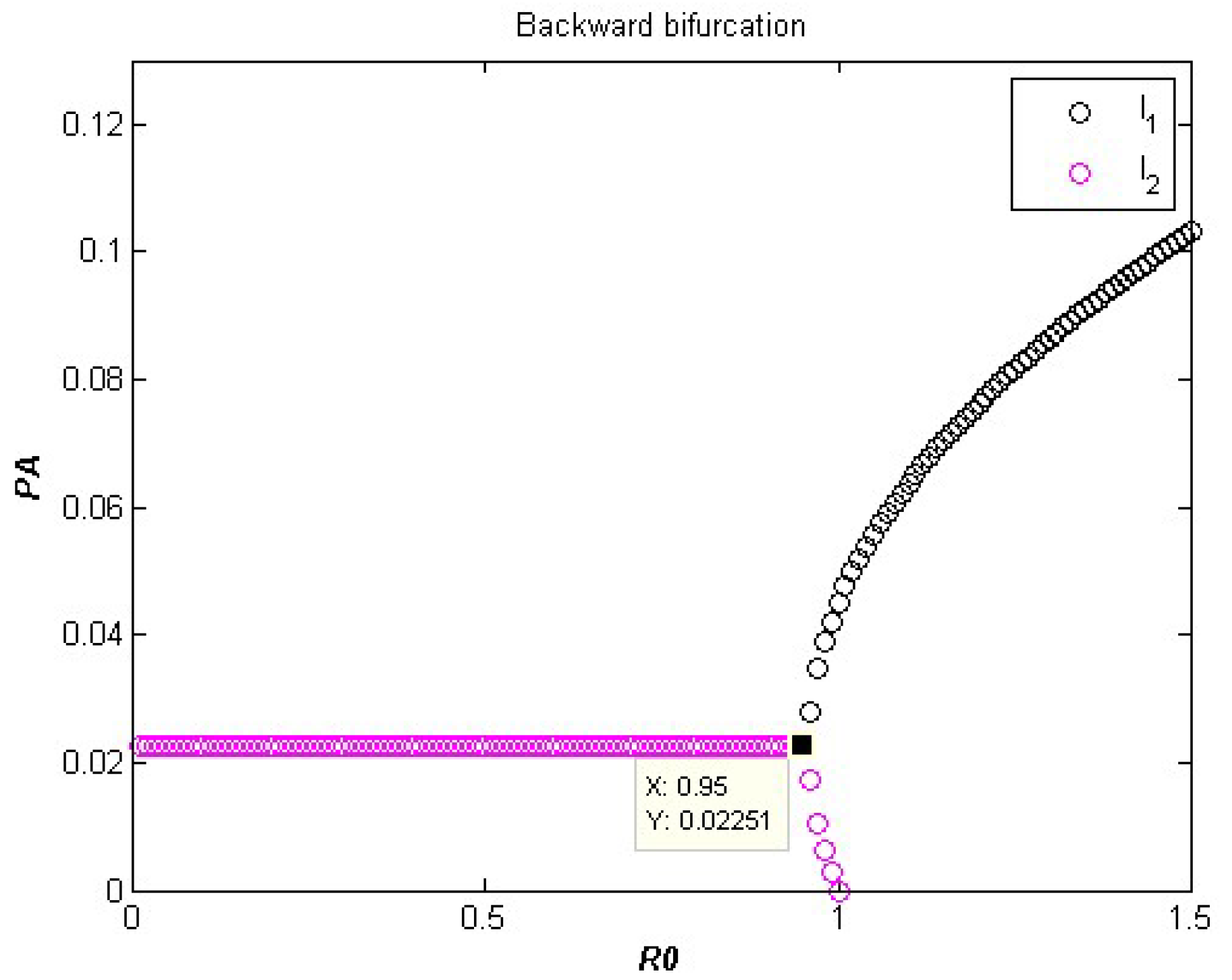
3. Backward Bifurcation

If the reproduction number $R_0$ > 1, then $P_A$ > 0, the system (1) exhibits a unique positive solution $E^{*}$. Now, on solving system (2), we have

$$F(P_A^{*})=b_2{P}_A^{*2}+b_1{P}_A^{*}+b_0$$

(10)

where,

$$\begin{array}{l}{b}_2={\beta }_1{\beta }_8({\beta }_5(L_2+\mu )-{\beta }_8({\beta }_4+\mu ))\\ b_1={\beta }_8(\mu +{\beta }_4)[{\beta }_1(L_1+\mu )+{\beta }_5(L_3+\mu )]-{\beta }_1{\beta }_5[(L_2+\mu )(L_3+\mu )+B{\beta }_8]-{\beta }_5^2(L_1+\mu )(L_2+\mu )\\ b_0=B{\beta }_1{\beta }_5^2\end{array}$$

Here, the coefficient $b_2<0$, and $b_0$ depends on the value of $R_0$. If $R_0<1$, then $b_0$ is positive and if $R_0>1$, then $b_0$ is negative. For $R_0>1$, Equation (10) has two roots, positive and negative.

For $b_1>0$, the system has endemic equilibria continuously depending on $R_0$; this shows that there exists an interval for $R_0$, which has two positive equilibria as follows:

$$I_1=\frac{-b_1-\sqrt{b_1{}^2-4b_2{b}_0}}{2b_2},I_2=\frac{-b_1+\sqrt{b_1{}^2-4b_2{b}_0}}{2b_2}$$

For Backward Bifurcation, setting $b_1{}^2-4b_2{b}_0=0$ and solving for critical points of $R_0$ gives

$$R_C=1-\frac{\begin{array}{l}[{\beta }_8(\mu +{\beta }_4)[{\beta }_1(L_1+\mu )+{\beta }_5(L_3+\mu )]-{\beta }_1{\beta }_5[(L_2+\mu )(L_3+\mu )\\ +B{\beta }_8]-{\beta }_5^2(L_1+\mu )(L_2+\mu ){]}^2((L_1+\mu )(L_2+\mu )(L_3+\mu )-B{\beta }_1{\beta }_8)\end{array}}{4({\beta }_1{\beta }_8({\beta }_5(L_2+\mu )-{\beta }_8({\beta }_4+\mu )))B{\beta }_2{\beta }_5^2(L_1+\mu )(L_2+\mu )(L_3+\mu )}$$

If $R_C<R_0$, then, equivalently, $b_1{}^2-4b_2{b}_0>0$ and backward bifurcation occur for the points of $R_0$, such that $R_C<R_0<1$ [22], as shown in the above Figure 2. Here, $R_C$= 0.95 is the critical value after which co-infection attains stability.

3.1. Sensitivity Analysis of $R_0$

In this section, sensitivity indices of $R_0$ with respect to different parameters are calculated as shown in

Table 2. Effect of Parameters on Sensitivity.

Parameter	Value	Observation
$B$	1	The transmission rate of HIV is directly proportional to birth rate.
${\beta }_1$	0.4925	The transmission rate of co-infection occurs at 49%.
${\beta }_2$	0.9013	Among HIV infectives, around 90% of them join the pre-AIDS stage.
${\beta }_3$	0.6084	Individuals moving toward medication can be increased further by creating awareness programs.
${\beta }_4$	0.5172
${\beta }_6$	0.77	77% of individuals in pre-AIDS class opt for medication.
${\beta }_7$	0.5022	From the pre-AIDS, class 50% of individuals undergo medication for TB disease.
${\beta }_8$	0.5075	Transmission occurs at the rate of 50% from the pre-AIDS class to pre-AIDS TB.
${\beta }_9$	0.724	The number of individuals in pre-AIDS class suffering from AIDS can be reduced if they take treatment while in pre-AIDS class.
${\beta }_{10}$	0.9967	The transmission rate of individuals from pre-AIDS TB stage to AIDS TB stage highly effects the sensitivity of $R_0$.
$\mu$	0.9793	Natural death rate cannot be removed completely even if the treatment is opted for in initial stage.

, using the formula ${\gamma }_{\alpha }^{R_0}=\frac{\partial R_0}{\partial \alpha }.\frac{\alpha }{R_0}$, where $\alpha$ is the model parameter. These indices show how crucial each parameter is to disease transmission.

The other parameters ${\beta }_5,{\beta }_{11},{\beta }_{12},{\mu }_D,{\mu }_{DTB}$ do not have any impact on the sensitivity of reproduction number.

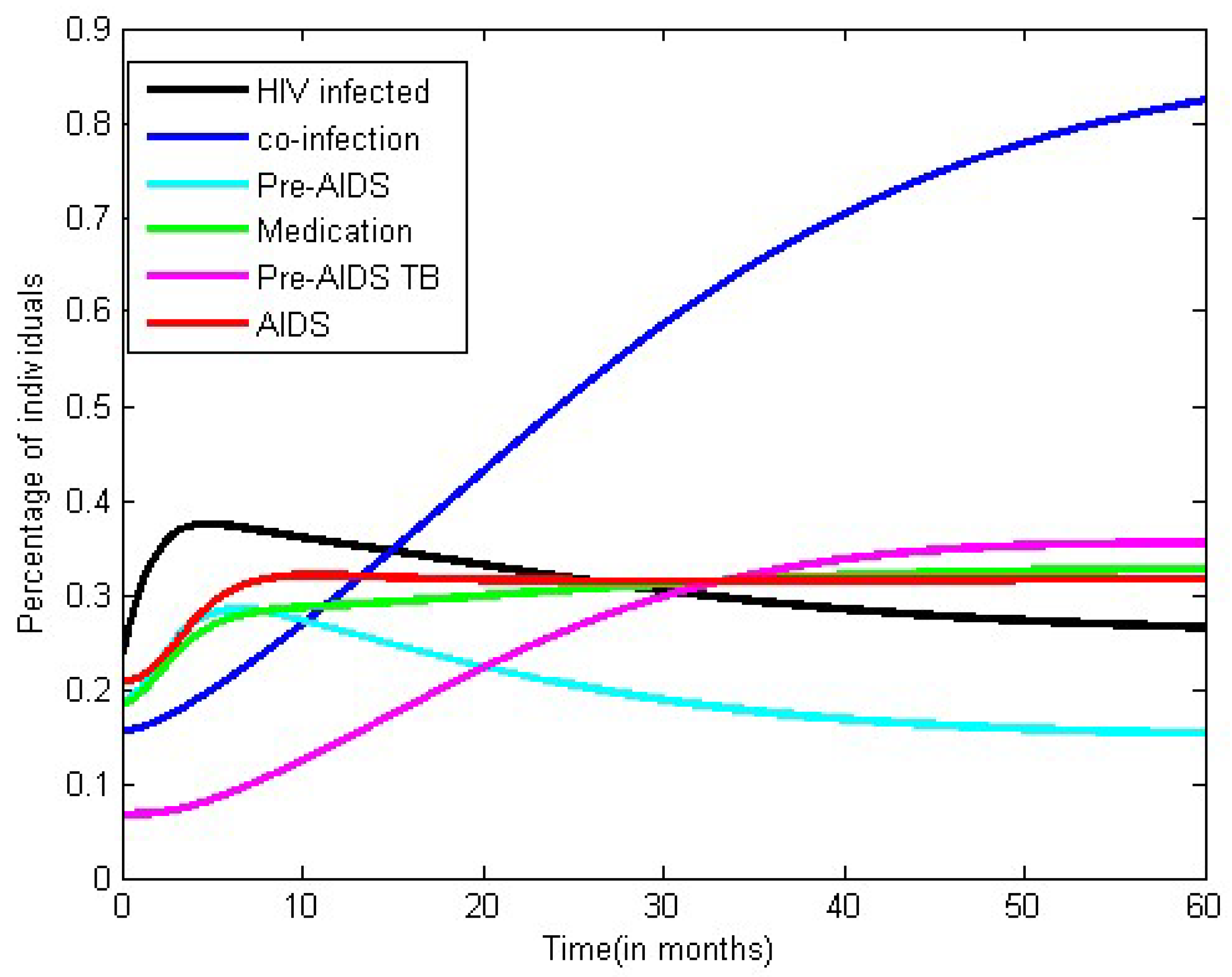
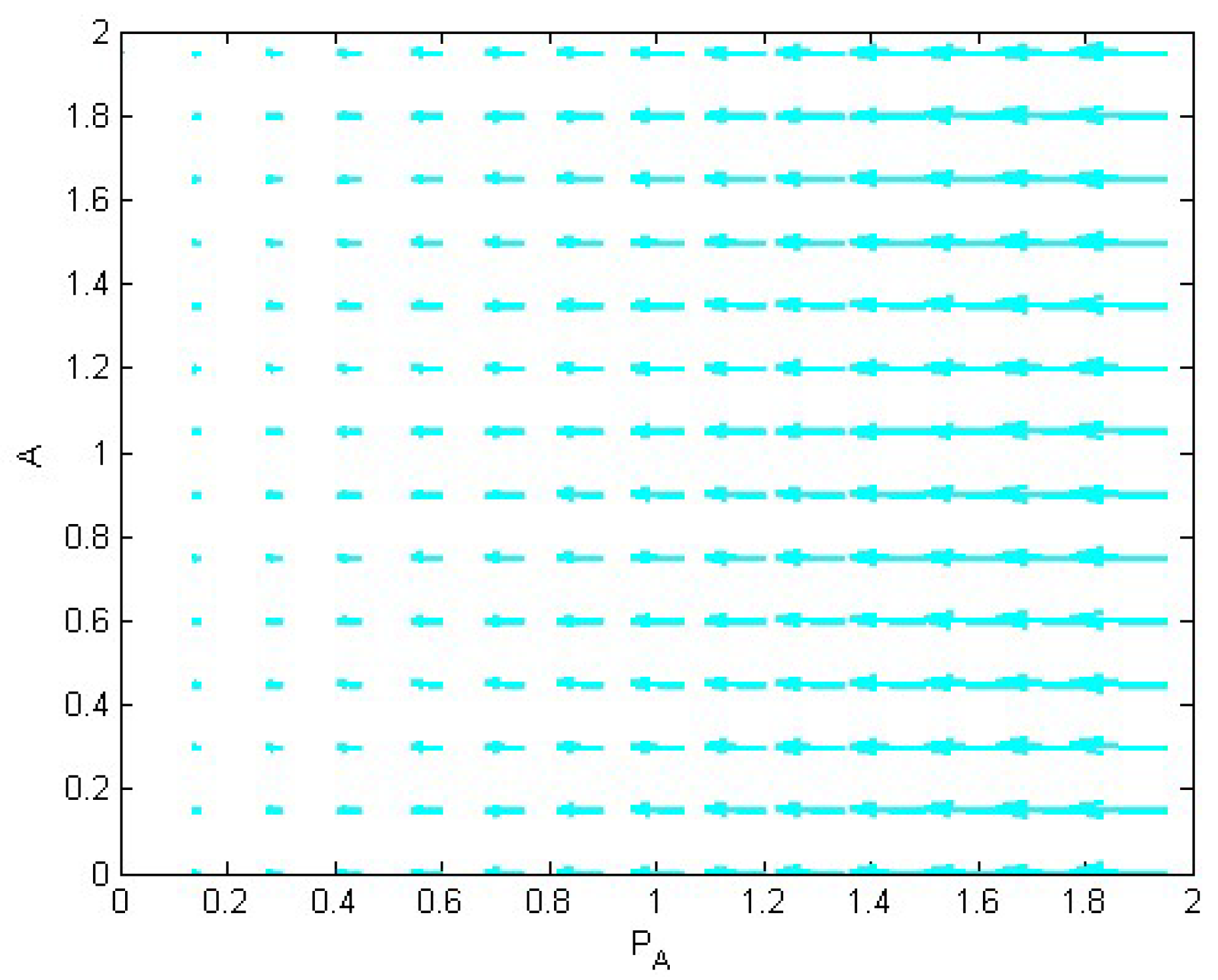
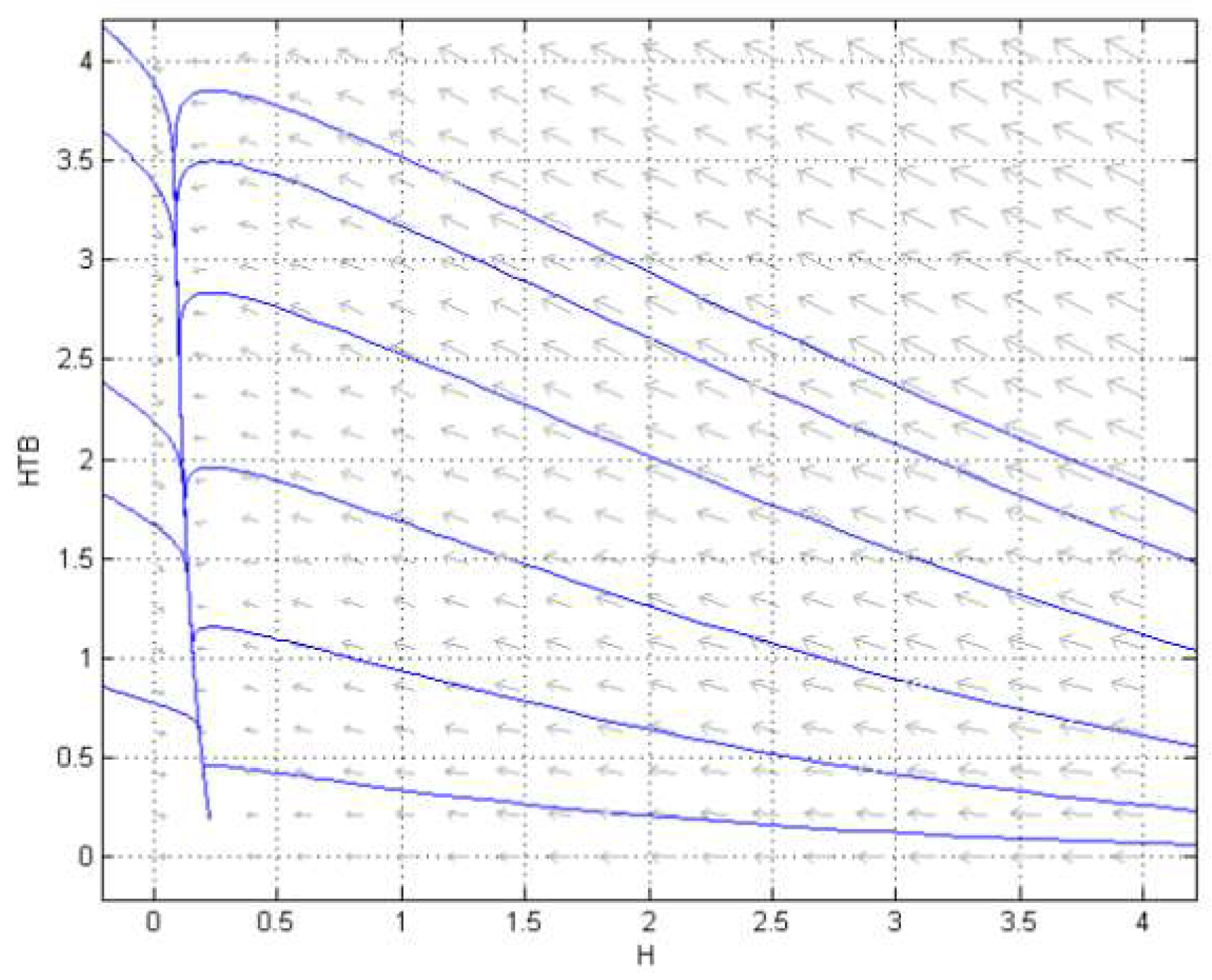
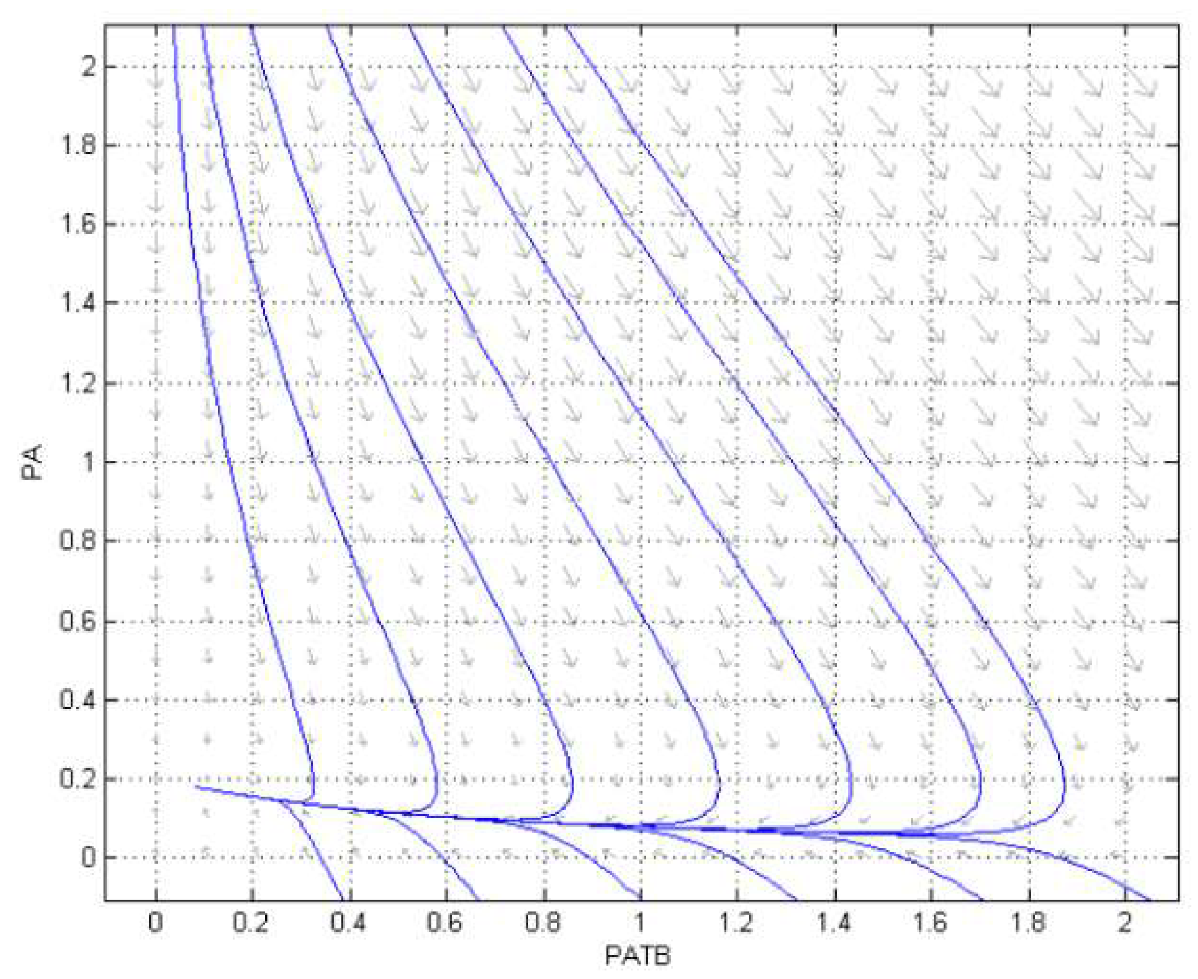
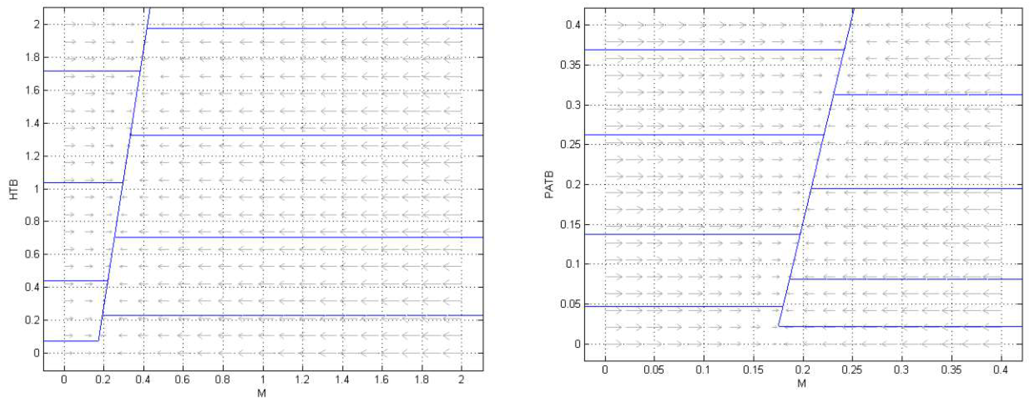
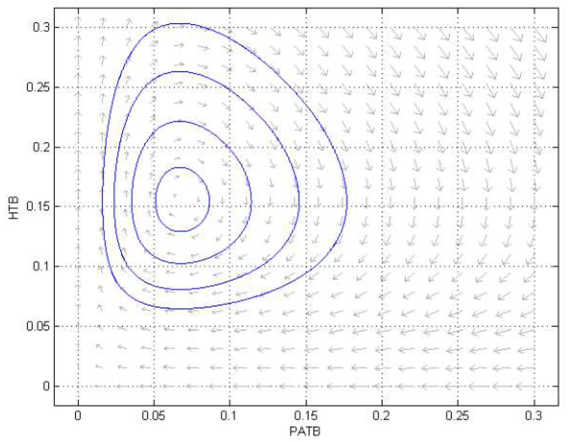
3.2. Numerical Simulation

From Figure 3 it can be observed that about 34% of the total HIV-infected population gets TB infection within 15 months. Approximately 30% of individuals infected with HIV go for treatment in 27 months. Co-infected individuals undergo treatment for TB in 11 months. Within 26 months, approximately 31% of HIV-infectives proceed to next stage, i.e., AIDS. About 22% of pre-AIDS infectives get TB infection and join pre-AIDS TB in 20 months. Individuals in the pre-AIDS class initially undergo medication then, due to ignorance or any other social reason, individuals leave the compartment and, after some time, joins the medication class again. Between approximately 1.7 and 4 months, individuals in the pre-AIDS class (not taking any kind of medication) suffer from AIDS, whereas those undergoing treatment get infected by AIDS within 28 months. This shows that medication is helpful. Even though it does not help the complete elimination of disease, the rate of disease spread can be controlled.

From Figure 4, we can conclude that individuals in Pre-AIDS class for a longer duration get AIDS at faster rate than the individuals who have just joined the pre-AIDS class.

Figure 5 indicates that individuals suffering from HIV suffer from TB also, and both the compartments stabilize after some time. Figure 6 shows that individuals in the pre-AIDS class also suffer from TB. The trajectory is stable.

Figure 7 shows the stability of the respective compartments.

Figure 8 shows that the newly HIV-TB infected individuals and individuals in Pre-AIDS TB class will oscillate cyclically. Here, neither compartment will die out completely nor they will grow indefinitely.

From Figure 9, it can be observed that, of the total population, 21% are HIV infected and 13% are HIV-TB infected, whereas the percentage of individuals in pre-AIDS and pre-AIDS TB stage is 16% and 6%, respectively. A total of 15% of the population undergoes treatment for both diseases. Since HIV-AIDS is not curable, even after taking treatment, 17% of cases lead to AIDS infections and 12% are infected by TB, moving towards the AIDS TB class.

4. Conclusions

In this paper, a mathematical model of HIV-TB considering the HIV-infected population is studied. Using data tabulated in Table 1, we have $R_0=2.262>1$, which shows the persistence of the disease in the society. HIV-AIDS cannot be eradicated completely from the infected population. Next, global stability is shown for the equilibrium points where there is no co-infection, and instances when there is no individual in the pre-AIDS TB class are shown using Castillo Chavez method. The equilibrium points where there is no co-infection and no individual in the pre-AIDS TB class proved to be globally unstable and is said to exhibit bifurcation. The endemic point is proven to be globally stable using Lyapunov function. Backward bifurcation analysis is studied, which indicates that a minimum of 95% of individuals join the pre-AIDS class. Numerical simulation is done to validate the model, which concludes that the medication plays a vital role in controlling disease spread. Here, we can observe that if treatment is provided at the initial stage of disease, its further progression can be prevented, and survival of individuals can be extended. The value of the reproduction number is highly affected by the rate at which individuals join the AIDS TB class. The pie-chart exhibits the distribution of the population in various compartments in the model.

References

1. Available online: https://www.who.int/news-room/fact-sheets/detail/hiv-aids (accessed on 3 January 2020).
2. Available online: https://www.who.int/tb/areas-of-work/tb-hiv/en/ (accessed on 3 January 2020).
3. Kwan, C.K.; Ernst, J.D. HIV and tuberculosis: A deadly human syndemic. Clin. Microbiol. Rev. 2011, 24, 351–376. [Google Scholar] [CrossRef] [PubMed] [Green Version]
4. Available online: https://www.avert.org/professionals/hiv-programming/hiv-tb-coinfection (accessed on 3 January 2020).
5. Kermack, W.O.; McKendrick, A.G. A contribution to the mathematical theory of epidemics. Proc. R. Soc. Lond. A Math. Phys. Char. 1927, 115, 700–721. [Google Scholar]
6. Cattani, C.; Ciancio, A. Qualitative analysis of second-order models of tumor—Immune system competition. Math. Comput. Model. 2008, 47, 1339–1355. [Google Scholar] [CrossRef]
7. Cattani, C.; Ciancio, A. Hybrid two scales mathematical tools for active particles modelling complex systems with learning hiding dynamics. Math. Models Methods Appl. Sci. 2007, 17, 171–187. [Google Scholar] [CrossRef]
8. Kirschner, D. Dynamics of Co-infection with M. tuberculosis and HIV-1. Theor. Popul. Biol. 1999, 55, 94–109. [Google Scholar] [CrossRef] [PubMed] [Green Version]
9. Naresh, R.; Tripathi, A. Modelling and analysis of HIV-TB co-infection in a variable size population. Math. Model. Anal. 2005, 10, 275–286. [Google Scholar] [CrossRef] [Green Version]
10. Huo, H.F.; Chen, R.; Wang, X.Y. Modelling and stability of HIV/AIDS epidemic model with treatment. Appl. Math. Model. 2016, 40, 6550–6559. [Google Scholar] [CrossRef]
11. Bhunu, C.P.; Garira, W.; Mukandavire, Z. Modeling HIV/AIDS and tuberculosis coinfection. Bull. Math. Biol. 2009, 71, 1745–1780. [Google Scholar] [CrossRef] [PubMed]
12. Roeger, L.I.W.; Feng, Z.; Castillo-Chavez, C. Modeling TB and HIV co-infections. Math. Biosci. Eng. 2009, 6, 815–837. [Google Scholar] [PubMed]
13. Singh, R.; Ali, S.; Jain, M. Epidemic model of HIV/AIDS transmission dynamics with different latent stages based on treatment. Am. J. Appl. Math. 2016, 4, 222–234. [Google Scholar] [CrossRef] [Green Version]
14. Silva, C.J.; Torres, D.F. Modeling TB-HIV syndemic and treatment. J. Appl. Math. 2014, 248407. [Google Scholar] [CrossRef] [Green Version]
15. Available online: https://aidsinfo.nih.gov/understanding-hiv-aids/fact-sheets/26/90/hiv-and-tuberculosis--tb- (accessed on 3 January 2020).
16. Diekmann, O.; Heesterbeek, J.A.P.; Metz, J.A. On the definition and the computation of the basic reproduction ratio R0 in models for infectious diseases in heterogeneous populations. J. Math. Biol. 1990, 28, 365–382. [Google Scholar] [CrossRef] [PubMed] [Green Version]
17. Freedman, H.I.; Ruan, S.; Tang, M. Uniform persistence and flows near a closed positively invariant set. J. Dyn. Differ. Equ. 1994, 6, 583–600. [Google Scholar] [CrossRef] [Green Version]
18. Thieme, H.R. Epidemic and demographic interaction in the spread of potentially fatal diseases in growing populations. Math. Biosci. 1992, 111, 99–130. [Google Scholar] [CrossRef]
19. Feng, Z.; Castillo-Chavez, C.; Capurro, A.F. A model for tuberculosis with exogenous reinfection. Theor. Popul. Biol. 2000, 57, 235–247. [Google Scholar] [CrossRef] [PubMed]
20. Castillo-Chavez, C.; Blower, S.; van den Driessche, P.; Kirschner, D.; Yakubu, A.A. (Eds.) Mathematical Approaches for Emerging and Reemerging Infectious Diseases: An Dntroduction; Springer Science & Business Media: Berlin, Germany.
21. LaSalle, J.P. The stability of dynamical systems. Soc. Ind. Appl. Math. 1976, 25. [Google Scholar] [CrossRef]
22. Khan, M.A.; Islam, S.; Khan, S.A. Mathematical modeling towards the dynamical interaction of leptospirosis. Appl. Math. Inf. Sci. 2014, 8, 1049–1056. [Google Scholar] [CrossRef] [Green Version]
Figure 1. Transmission of individuals in different compartments.
Axioms 09 00029 g001
Figure 2. Pre-AIDS class at equilibria versus R 0 .
Axioms 09 00029 g002
Figure 3. Transmission of HIV–TB co-infection.
Axioms 09 00029 g003
Figure 4. Intensity of pre-AIDS class versus AIDS class.
Axioms 09 00029 g004
Figure 5. Behavior of H v/s HTB.
Axioms 09 00029 g005
Figure 6. Trajectory of P A T B and P A .
Axioms 09 00029 g006
Figure 7. Phase transition plot of M with H T B and P A T B .
Axioms 09 00029 g007
Figure 8. Phase transition of co-infection and pre-stage of co-infection.
Axioms 09 00029 g008
Figure 9. Percentage wise distribution of different compartments.
Axioms 09 00029 g009