Article

Stability of Equilibria of Rumor Spreading Model under Stochastic Perturbations

Department of Mathematics, Ariel University, Ariel 40700, Israel
Axioms 2020, 9(1), 24; https://doi.org/10.3390/axioms9010024
Submission received: 2 February 2020 / Revised: 11 February 2020 / Accepted: 11 February 2020 / Published: 18 February 2020

Abstract

:
The known mathematical model of rumor spreading, which is described by a system of four nonlinear differential equations and is very popular in research, is considered. It is supposed that the considered model is influenced by stochastic perturbations that are of the type of white noise and are proportional to the deviation of the system state from its equilibrium point. Sufficient conditions of stability in probability for each from the five equilibria of the considered model are obtained by virtue of the Routh–Hurwitz criterion and the method of linear matrix inequalities (LMIs). The obtained results are illustrated by numerical analysis of appropriate LMIs and numerical simulations of solutions of the considered system of stochastic differential equations. The research method can also be used in other applications for similar nonlinear models with the order of nonlinearity higher than one.

1. Introduction

There are two classes of mathematical models of the type of epidemics: medical epidemics (see, for instance, the so-called SIR-epidemic model [1,2,3]) and different social epidemics (see, for instance, the alcohol consumption model [4] or the model of obesity epidemic [5]). During the last two decades, the rumor spreading model, that is an epidemic of the social type too, is extremely popular in research (see, [6,7,8,9,10,11,12,13,14,15,16,17,18,19,20,21,22,23,24,25,26,27,28,29]). Following [26], we will consider the rumor spreading model (the so-called I2SR-model) in the form
I ˙ ( t ) = p λ 1 I ( t ) S 1 ( t ) λ 2 I ( t ) S 2 ( t ) q I ( t ) , S ˙ 1 ( t ) = λ 1 I ( t ) S 1 ( t ) + α S 2 ( t ) δ 1 S 1 ( t ) R ( t ) q S 1 ( t ) , S ˙ 2 ( t ) = λ 2 I ( t ) S 2 ( t ) α S 2 ( t ) δ 2 S 2 ( t ) R ( t ) q S 2 ( t ) , R ˙ ( t ) = δ 1 S 1 ( t ) R ( t ) + δ 2 S 2 ( t ) R ( t ) q R ( t ) ,
where I ( t ) , S 1 ( t ) , S 2 ( t ) , R ( t ) are respectively the density of ignorants, the low rate of active spreaders, the high rate of active spreaders and stiflers at time t, p , q , α , δ 1 , δ 2 , λ 1 , λ 2 are positive parameters.
Please note that the sense of the parameters p , q , α , δ 1 , δ 2 , λ 1 , λ 2 that are used in the rumor spreading model (1) are described in [26]. We will consider the system (1) as a mathematical object and show how stability of nonlinear mathematical models of the similar type can be investigated under influence of stochastic perturbations. In particular, we will consider here the simple parameters λ i and δ i unlike from [26], where these parameters are considered in the form of the product of two parameters: λ i k ¯ and δ i k ¯ , i = 1 , 2 . We will not suppose in the general case as it is made in [26] that p = q and δ 1 = δ 2 . We will correct also some errors and inaccuracies which there are in [26]. For example, in [26] it is supposed that λ 2 > λ 1 (p. 856) but in the numerical examples the following values are used: λ 1 = 0.05 and λ 2 = 0.007 or λ 2 = 0.003 (p. 862), all equilibria and stability conditions are obtained under the assumption δ 1 = δ 2 = δ (p. 857) but in the numerical examples one can see δ 1 = 0.007 and δ 2 = 0.59 (p. 862) or δ 2 = 0.009 (p. 863) and so on.
The purpose of the proposed research is to calculate of equilibria of the system (1) and to obtain stability conditions for each from these equilibria under assumption that the system is exposed to stochastic perturbations. Sufficient conditions of stability in probability for each from the five equilibria of the considered model are obtained by virtue of the Routh–Hurwitz criterion [30] and the method of linear matrix inequalities (LMIs) [31,32]. The proposed research method can be used for a lot of other similar nonlinear models in different applications.

2. Equilibria of the Model

Equilibria E = ( I * , S 1 * , S 2 * , R * ) of the model (1) are defined by the system of algebraic equations
( λ 1 S 1 + λ 2 S 2 + q ) I = p , ( δ 1 R λ 1 I + q ) S 1 = α S 2 , ( δ 2 R λ 2 I + α + q ) S 2 = 0 , ( δ 1 S 1 + δ 2 S 2 q ) R = 0 ,
that follows from (1) by the condition that I ( t ) , S 1 ( t ) , S 2 ( t ) , R ( t ) are constants.
Please note that the solution of the system (2) is not unique. Solving the system (2) gives the following five equilibria E i = ( I i * , S 1 i * , S 2 i * , R i * ) , i = 0 , , 4 , where (see Appendix A.1)
E 0 = ( I 0 * , 0 , 0 , 0 ) , I 0 * = p q ; E 1 = ( I 1 * , S 11 * , 0 , 0 ) , I 1 * = q λ 1 , S 11 * = p q q λ 1 ; E 2 = ( I 2 * , S 12 * , 0 , R 2 * ) , I 2 * = p δ 1 q ( δ 1 + λ 1 ) , S 12 * = q δ 1 , R 2 * = p λ 1 q ( δ 1 + λ 1 ) q δ 1 ; E 3 = ( I 3 * , S 13 * , S 23 * , 0 ) , I 3 * = α + q λ 2 , S 13 * = α ( p λ 2 q ( α + q ) ) q ( λ 2 λ 1 ) ( α + q ) , S 23 * = ( q ( λ 2 λ 1 ) α λ 1 ) ( p λ 2 q ( α + q ) ) λ 2 q ( λ 2 λ 1 ) ( α + q ) ; E 4 = ( I 4 * , S 14 * , S 24 * , R 4 * ) , if ( δ 2 δ 1 ) ( λ 2 δ 1 λ 1 δ 2 ) 0 then S 14 * is a positive root of the quadratic equation S 1 2 ν 1 S 1 + ν 2 = 0 , ν 1 = q α + p δ 2 q ( δ 2 δ 1 ) + q ( λ 2 + δ 2 ) λ 2 δ 1 λ 1 δ 2 , ν 2 = α q ( λ 2 + δ 2 ) ( δ 2 δ 1 ) ( λ 2 δ 1 λ 1 δ 2 ) , S 14 * = α q 2 ( δ + λ 2 ) δ ( λ 2 λ 1 ) ( q α + p δ ) if δ 2 = δ 1 = δ , λ 2 > λ 1 ,    α δ 2 δ 1 if λ 2 δ 1 = λ 1 δ 2 , δ 2 > δ 1 , S 24 * = 1 δ 2 ( q δ 1 S 14 * ) , I 4 * = p λ 1 S 14 * + λ 2 S 24 * + q , R 4 * = λ 2 I 4 * α q δ 2 , S 14 * < q δ 1 , I 4 * > α + q λ 2 .
It is supposed that all nonzero elements of all equilibria are positive.
Putting N ( t ) = I ( t ) + S 1 ( T ) + S 2 ( t ) + R ( t ) and summing all equations of the system (1), we obtain
N ˙ ( t ) = p q N ( t ) , N ( t ) = N ( 0 ) p q e q t + p q , lim t N ( t ) = p q .
In accordance with (4) for all equilibria we have
N * = I i * + S 1 i * + S 2 i * + R i * = p q , i = 0 , , 4 .

3. Stochastic Perturbations, Centralization, and Linearization

Let us suppose that the system (1) is exposed to stochastic perturbations which are directly proportional to the deviation of the system (1) state ( I ( t ) , S 1 ( t ) , S 2 ( t ) , R ( t ) ) from the equilibrium ( I * , S 1 * , S 2 * , R * ) and are of the type of white noise ( w ˙ 0 ( t ) , w ˙ 1 ( t ) , w ˙ 2 ( t ) , w ˙ 3 ( t ) ), where ( w 0 ( t ) , w 1 ( t ) , w 2 ( t ) , w 3 ( t ) ) are mutually independent standard Wiener processes. Therefore, we obtain the following system of the Ito stochastic differential equations [33]
I ˙ ( t ) = p λ 1 I ( t ) S 1 ( t ) λ 2 I ( t ) S 2 ( t ) q I ( t ) + σ 0 ( I ( t ) I * ) w ˙ 0 ( t ) , S ˙ 1 ( t ) = λ 1 I ( t ) S 1 ( t ) + α S 2 ( t ) δ 1 S 1 ( t ) R ( t ) q S 1 ( t ) + σ 1 ( S 1 ( t ) S 1 * ) w ˙ 1 ( t ) , S ˙ 2 ( t ) = λ 2 I ( t ) S 2 ( t ) α S 2 ( t ) δ 2 S 2 ( t ) R ( t ) q S 2 ( t ) + σ 2 ( S 2 ( t ) S 2 * ) w ˙ 2 ( t ) , R ˙ ( t ) = δ 1 S 1 ( t ) R ( t ) + δ 2 S 2 ( t ) R ( t ) q R ( t ) + σ 3 ( R ( t ) R * ) w ˙ 3 ( t ) .
Please note that the equilibrium ( I * , S 1 * , S 2 * , R * ) of the deterministic system (1) is also a solution of the system with stochastic perturbations (6).
Let ( I * , S 1 * , S 2 * , R * ) be one of the equilibria of the system (1). Putting in (6) I ( t ) = y 0 ( t ) + I * , S 1 ( t ) = y 1 ( t ) + S 1 * , S 2 ( t ) = y 2 ( t ) + S 2 * , R ( t ) = y 3 ( t ) + R * , we obtain
y ˙ 0 ( t ) = p ( y 0 ( t ) + I * ) [ λ 1 ( y 1 ( t ) + S 1 * ) + λ 2 ( y 2 ( t ) + S 2 * ) + q ] + σ 0 y 0 ( t ) w ˙ 0 ( t ) , y ˙ 1 ( t ) = ( y 1 ( t ) + S 1 * ) [ λ 1 ( y 0 ( t ) + I * ) δ 1 ( y 3 ( t ) + R * ) q ] + α ( y 2 ( t ) + S 2 * ) + σ 1 y 1 ( t ) w ˙ 1 ( t ) , y ˙ 2 ( t ) = ( y 2 ( t ) + S 2 * ) [ λ 2 ( y 0 ( t ) + I * ) δ 2 ( y 3 ( t ) + R * ) α q ] + σ 2 y 2 ( t ) w ˙ 2 ( t ) , y ˙ 3 ( t ) = ( y 3 ( t ) + R * ) [ δ 1 ( y 1 ( t ) + S 1 * ) + δ 2 ( y 2 ( t ) + S 2 * ) q ] + σ 3 y 3 ( t ) w ˙ 3 ( t ) .
It is clear that stability of the zero solution of the system (7) is equivalent to stability of the equilibrium ( I * , S 1 * , S 2 * , R * ) of the system (6).
Removing from the system (7) nonlinear terms and using the system for equilibria (2) we obtain the linear part of the system (7)
z ˙ 0 ( t ) = p ( I * ) 1 z 0 ( t ) λ 1 I * z 1 ( t ) λ 2 I * z 2 ( t ) + σ 0 z 0 ( t ) w ˙ 0 ( t ) , z ˙ 1 ( t ) = λ 1 S 1 * z 0 ( t ) ( q + δ 1 R * λ 1 I * ) z 1 ( t ) + α z 2 ( t ) δ 1 S 1 * z 3 ( t ) + σ 1 z 1 ( t ) w ˙ 1 ( t ) , z ˙ 2 ( t ) = λ 2 S 2 * z 0 ( t ) ( α + q λ 2 I * + δ 2 R * ) z 2 ( t ) δ 2 S 2 * z 3 ( t ) + σ 2 z 2 ( t ) w ˙ 2 ( t ) , z ˙ 3 ( t ) = δ 1 R * z 1 ( t ) + δ 2 R * z 2 ( t ) ( q δ 1 S 1 * δ 2 S 2 * ) z 3 ( t ) + σ 3 z 3 ( t ) w ˙ 3 ( t ) .
Let us present the system (8) in the matrix form
d z ( t ) = A z ( t ) d t + C ( z ( t ) ) d w ( t ) ,
where z ( t ) = ( z 0 ( t ) , z 1 ( t ) , z 2 ( t ) , z 3 ( t ) ) , w ( t ) = ( w 0 ( t ) , w 1 ( t ) , w 2 ( t ) , w 3 ( t ) ) , C ( z ( t ) ) = d i a g ( σ 0 z 0 ( t ) , , σ 3 z 3 ( t ) ) ,
A = [ p ( I * ) 1 λ 1 I * λ 2 I *    0 λ 1 S 1 * ( q + δ 1 R * λ 1 I * ) α δ 1 S 1 * λ 2 S 2 * 0 ( α + q λ 2 I * + δ 2 R * ) δ 2 S 2 *     0 δ 1 R * δ 2 R * ( q δ 1 S 1 * δ 2 S 2 * ) ] .
Remark 1.
The order of nonlinearity of the nonlinear system (7) is higher than one. For systems of such type a sufficient condition for asymptotic mean square stability of the zero solution of its linear part (9) provides stability in probability of the zero solution of the initial nonlinear system (7) [30]. Therefore, a sufficient condition for asymptotic mean square stability of the zero solution of the linear Equation (9) provides stability in probability of the equilibrium ( I * , S 1 * , S 2 * , R * ) of the initial system (6).
Following Remark 1, below we will have sufficient conditions for asymptotic mean square stability of the zero solution of the linear Equation (9) for each from the equilibria (3).

4. Stability of the Equilibria

Consider some definitions and statements that will be used below [30].
Definition 1.
The zero solution of the system (7) is called stable in probability if for any ε 1 > 0 and ε 2 > 0 there exists δ > 0 such that the solution y ( t ) = ( y 0 ( t ) , y 1 ( t ) , y 2 ( t ) , y 3 ( t ) ) of the system (7) satisfies the condition P { sup t 0 | y ( t ) | > ε 1 } < ε 2 provided that P { | y ( 0 ) | < δ } = 1 .
Definition 2.
The zero solution of the system (9) is called:
-
mean square stable if for each ε > 0 there exists a δ > 0 such that E | z ( t ) | 2 < ε , t 0 , provided that E | z ( 0 ) | 2 < δ ;
-
asymptotically mean square stable if it is mean square stable and the solution z ( t ) of Equation (9) satisfies the condition lim t E | z ( t ) | 2 = 0 provided that E | z ( 0 ) | 2 < .
The generator L of the Ito stochastic differential Equation (9) is defined on the functions V ( t , z ) which have one continuous derivative with respect to t ( V t ), two continuous derivatives ( V and 2 V ) with respect to z and has the form [30,33]
L V ( t , z ( t ) ) = V t ( t , z ( t ) ) + V ( t , z ( t ) ) A z ( t ) + 1 2 T r [ C ( z ( t ) ) 2 V ( t , z ( t ) ) C ( z ( t ) ) ] .
Theorem 1.
Let there exist a function V ( t , z ) with continuous derivatives V t , V , 2 V , positive constants c 1 , c 2 , c 3 , such that the following conditions hold:
E V ( t , z ( t ) ) c 1 E | z ( t ) | 2 , E V ( 0 , z ( 0 ) ) c 2 E | z ( 0 ) | 2 , E L V ( t , z ( t ) ) c 3 E | z ( t ) | 2 .
Then the zero solution of Equation (9) is asymptotically mean square stable.
Lemma 1.
Let there exist a positive definite matrix P = p i j ( i , j = 1 , 2 , 3 , 4 ) such that the matrix (10) with the equilibrium ( I * , S 1 * , S 2 * , R * ) satisfies the linear matrix inequality (LMI)
P A + A P + P σ < 0 , P σ = d i a g { p 11 σ 0 2 , , p 44 σ 3 2 } .
Then the equilibrium ( I * , S 1 * , S 2 * , R * ) of the system (6) is stable in probability.
Proof. 
For the function V ( t , z ) = z P z from (11) and LMI (12) for some c > 0 we have
L V ( t , z ( t ) ) = 2 z ( t ) P A z ( t ) + T r [ C ( z ( t ) ) P C ( z ( t ) ) ] = z ( t ) ( P A + A P + P σ ) z ( t ) c | z ( t ) | 2 .
From Theorem 1 it follows that the zero solution of Equation (9) is asymptotically mean square stable. Via Remark 1 one can conclude that the equilibrium ( I * , S 1 * , S 2 * , R * ) of the system (6) is stable in probability. The proof is completed. □
Note to satisfy the LMI (12) the matrix A must be the Hurwitz matrix [30,31].
Definition 3.
The trace of the k - th order of a n × n -matrix A = a i j is defined as follows:
T k = 1 i 1 < < i k n a i 1 i 1 a i 1 i k a i k i 1 a i k i k , k = 1 , , n .
Here, in particular, T 1 = T r ( A ) , T n = det ( A ) , T n 1 = i = 1 n A i i , where A i i is the algebraic complement of the diagonal element a i i of the matrix A.
Lemma 2.
[30,31] Let T k , k = 1 , 2 , 3 , 4 , be the trace of the k-th order of a 4 × 4 -matrix A. The matrix A is the Hurwitz matrix if and only if
T 1 < 0 , T 1 T 2 < T 3 < 0 , 0 < T 1 2 T 4 < ( T 1 T 2 T 3 ) T 3 .
A 3 × 3 -matrix A is the Hurwitz matrix if and only if first two conditions (13) hold.
In general, the LMI (12) for each equilibrium (3) must be numerically investigated via MATLAB. However, in some particular cases this process can be simplified and analytical conditions can be obtained. Below it is shown in investigation of stability of the equilibria (3).

4.1. Stability of the Equilibrium E 0 = ( p q , 0 , 0 , 0 )

Theorem 2.
If
1 λ 1 > p q 2 , 1 λ 2 1 + α q > p q 2 ,
and
σ 0 2 < 2 q , σ 1 2 < 2 q λ 1 p q , σ 2 2 < 2 α + q λ 2 p q , σ 3 2 < 2 q ,
then the equilibrium E 0 is stable in probability.
Proof. 
For the equilibrium E 0 = p q , 0 , 0 , 0 the system (8) takes the form
z ˙ 0 ( t ) = q z 0 ( t ) λ 1 p q 1 z 1 ( t ) λ 2 p q 1 z 2 ( t ) + σ 0 z 0 ( t ) w ˙ 0 ( t ) , z ˙ 1 ( t ) = ( q λ 1 p q 1 ) z 1 ( t ) + α z 2 ( t ) + σ 1 z 1 ( t ) w ˙ 1 ( t ) , z ˙ 2 ( t ) = ( α + q λ 2 p q 1 ) z 2 ( t ) + σ 2 z 2 ( t ) w ˙ 2 ( t ) , z ˙ 3 ( t ) = q z 3 ( t ) + σ 3 z 3 ( t ) w ˙ 3 ( t ) .
The conditions (14) provide negativity of the coefficients before z 1 ( t ) and z 2 ( t ) in the second and the third equations (16). It is known [30] that the last two inequalities (15) are the necessary and sufficient conditions for asymptotic mean square stability of the zero solutions of the last two equations in (16) which do not depend on z 0 ( t ) and z 1 ( t ) and can be considered separately. Since lim t E z 2 2 ( t ) = 0 then the system of first two Equation (16) for z 0 ( t ) and z 1 ( t ) can be considered without the process z 2 ( t ) , i.e.,
z ˙ 0 ( t ) = q z 0 ( t ) λ 1 p q 1 z 1 ( t ) + σ 0 z 0 ( t ) w ˙ 0 ( t ) , z ˙ 1 ( t ) = ( q λ 1 p q 1 ) z 1 ( t ) + σ 1 z 1 ( t ) w ˙ 1 ( t ) .
Via Remark A2 (see Appendix A.2) the first two inequalities (15) are sufficient for asymptotic mean square stability of the zero solution of the system (17). Therefore, the conditions (14), (15) provide asymptotic mean square stability of the zero solution of the system (16) and via Remark 1 stability in probability of the equilibrium E 0 of the system (6). The proof is completed. □
Remark 2.
One can check that by the conditions (14) and (15) the matrix
A = [ q λ 1 p q 1 λ 2 p q 1 0 0 ( q λ 1 p q 1 ) α 0 0 0 ( α + q λ 2 p q 1 ) 0 0 0 0 q ]
of the system (16) satisfies the conditions (13).
Example 1.
Put
α = 0.4 , λ 1 = 0.5 , λ 2 = 0.7 , δ 1 = δ 2 = 0.2 , p = 0.8 , q = 0.7 , σ 0 = 1.18 , σ 1 = 0.50 , σ 2 = 0.77 , σ 3 = 1.18 .
By these values of the parameters the conditions (14) and (15) hold:
1 λ 1 = 2 > p q 2 = 1.63 , 1 λ 2 1 + α q = 2.24 > p q 2 = 1.63 , σ 0 2 = 1.3924 < 2 q = 1.4 , σ 1 2 = 0.25 < 2 q λ 1 p q = 0.257 , σ 2 2 = 0.5929 < 2 α + q λ 2 p q = 0.6 , σ 3 2 = 1.3924 < 2 q = 1.4 .
Using MATLAB it was shown that by the values of the parameters (19) the matrix (18) satisfies the LMI (12). The conditions (13) with
T 1 = 1.8286 < 0 , T 2 = 1.1286 > 0 , T 3 = 0.2640 < 0 , T 4 = 0.0189 > 0 , T 3 T 1 T 2 = 1.7997 > 0 , ( T 1 T 2 T 3 ) T 3 T 1 2 T 4 = 0.4119 > 0 ,
hold too. Therefore, the equilibrium E 0 is stable in probability.
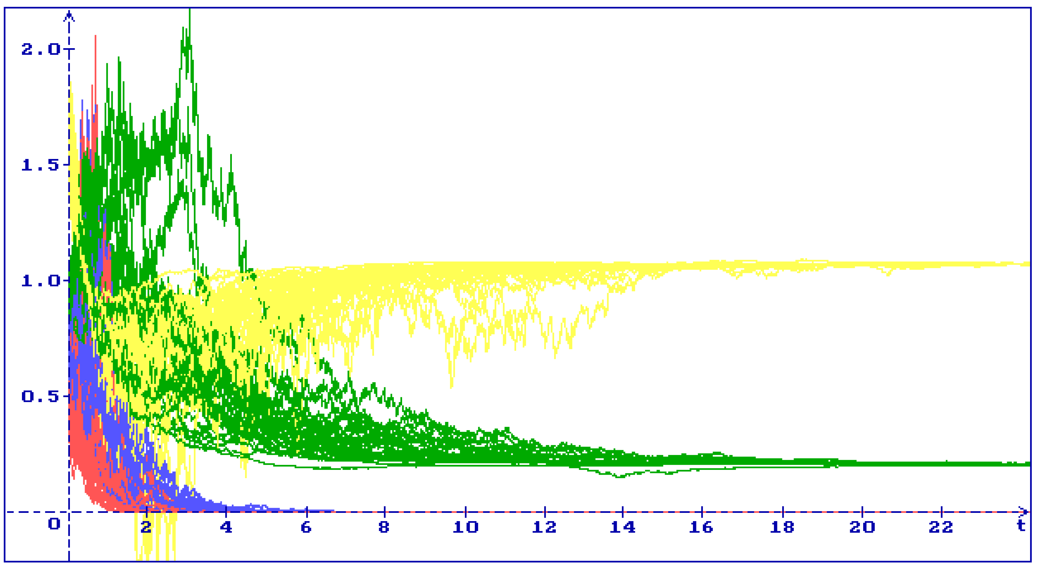
In Figure 1 one can see 30 trajectories of the system (6) solution for the equilibrium E 0 with the initial condition I ( 0 ) = 1.7 , S 1 ( 0 ) = 0.9 , S 2 ( 0 ) = 0.7 , R ( 0 ) = 0.5 : all trajectories I ( t ) (yellow), S 1 ( t ) (green), S 2 ( t ) (blue), R ( t ) (red) converge to the equilibrium E 0 = ( I * , S 1 * , S 2 * , R * ) = ( 1.1429 , 0 , 0 , 0 ) .

4.2. Stability of the Equilibrium E 1 = q λ 1 , p q q λ 1 , 0 , 0

Theorem 3.
If
1 λ 1 + 1 δ 1 > p q 2 > 1 λ 1 , 1 λ 2 1 + α q > 1 λ 1 ,
and
σ 0 2 < 2 p λ 1 q , σ 1 2 < 2 p λ 1 q + q p λ 1 1 q 2 p λ 1 1 , σ 2 2 < 2 α + q q λ 2 λ 1 , σ 3 2 < 2 q δ 1 p q q λ 1 ,
then the equilibrium E 1 is stable in probability.
Proof. 
For the equilibrium E 1 = q λ 1 , p q q λ 1 , 0 , 0 the system (8) takes the form
z ˙ 0 ( t ) = p q 1 λ 1 z 0 ( t ) q z 1 ( t ) q λ 2 λ 1 1 z 2 ( t ) + σ 0 z 0 ( t ) w ˙ 0 ( t ) , z ˙ 1 ( t ) = λ 1 p q q λ 1 z 0 ( t ) + α z 2 ( t ) δ 1 p q q λ 1 z 3 ( t ) + σ 1 z 1 ( t ) w ˙ 1 ( t ) , z ˙ 2 ( t ) = ( α + q q λ 2 λ 1 1 ) z 2 ( t ) + σ 2 z 2 ( t ) w ˙ 2 ( t ) , z ˙ 3 ( t ) = q δ 1 p q q λ 1 z 3 ( t ) + σ 3 z 3 ( t ) w ˙ 3 ( t ) .
The conditions (20) provide positivity of the nonzero component of the equilibrium E 1 and negativity of the coefficients before z 2 ( t ) and z 3 ( t ) in the last two equations (22). The last two inequalities (21) are the necessary and sufficient conditions for asymptotic mean square stability of the zero solutions of last two equations in (22) [30] which do not depend on z 0 ( t ) and z 1 ( t ) and can be considered separately. Since lim t E z 2 2 ( t ) = 0 and lim t E z 3 2 ( t ) = 0 then the system of first two Equation (22) for z 0 ( t ) and z 1 ( t ) can be considered without the processes z 2 ( t ) , z 3 ( t ) , i.e.,
z ˙ 0 ( t ) = p q 1 λ 1 z 0 ( t ) q z 1 ( t ) + σ 0 z 0 ( t ) w ˙ 0 ( t ) , z ˙ 1 ( t ) = λ 1 p q q λ 1 z 0 ( t ) + σ 1 z 1 ( t ) w ˙ 1 ( t ) .
Via Remark A2 (see Appendix A.2) first two inequalities (21) are sufficient for asymptotic mean square stability of the zero solution of the system (23). Therefore, the conditions (20) and (21) provide asymptotic mean square stability of the zero solution of the system (22) and via Remark 1 stability in probability of the equilibrium E 1 of the system (6). The proof is completed. □
Remark 3.
One can check that by the conditions (20) and (21) the matrix
A = [ p q 1 λ 1 q q λ 2 λ 1 1 0 λ 1 p q q λ 1 0 α δ 1 p q q λ 1 0 0 ( α + q q λ 2 λ 1 1 ) 0 0 0 0 q δ 1 p q q λ 1 ]
of the system (22) satisfies the conditions (13).
Example 2.
Put
α = 0.4 , λ 1 = 0.65 , λ 2 = 0.75 , δ 1 = δ 2 = 0.2 , p = 0.9 , q = 0.7 , σ 0 = 1.01 , σ 1 = 0.41 , σ 2 = 0.76 , σ 3 = 1.14 .
By these values of the parameters the conditions (20) and (21) hold:
1 λ 1 + 1 δ 1 = 6.538 > p q 2 = 1.837 > 1 λ 1 = 1.538 , 1 λ 2 1 + α q = 2.095 > 1 λ 1 = 1.538 , σ 0 2 = 1.0201 < 2 p λ 1 q < 1.671 , σ 1 2 = 0.1681 < 2 p λ 1 q + q p λ 1 1 q 2 p λ 1 1 = 0.2001 , σ 2 2 = 0.5776 < 2 α + q q λ 2 λ 1 = 0.5846 , σ 3 2 = 1.2996 < 2 q δ 1 p q q λ 1 = 1.3165 .
Using MATLAB it was shown that by the values of the parameters (25) the matrix (24) satisfies the LMI (12), the conditions (13) with
T 1 = 1.7863 < 0 , T 2 = 1.0818 > 0 , T 3 = 0.2511 < 0 , T 4 = 0.0183 > 0 , T 3 T 1 T 2 = 1.6813 > 0 , ( T 1 T 2 T 3 ) T 3 T 1 2 T 4 = 0.3638 > 0 ,
hold too. Therefore, the equilibrium E 1 is stable in probability.
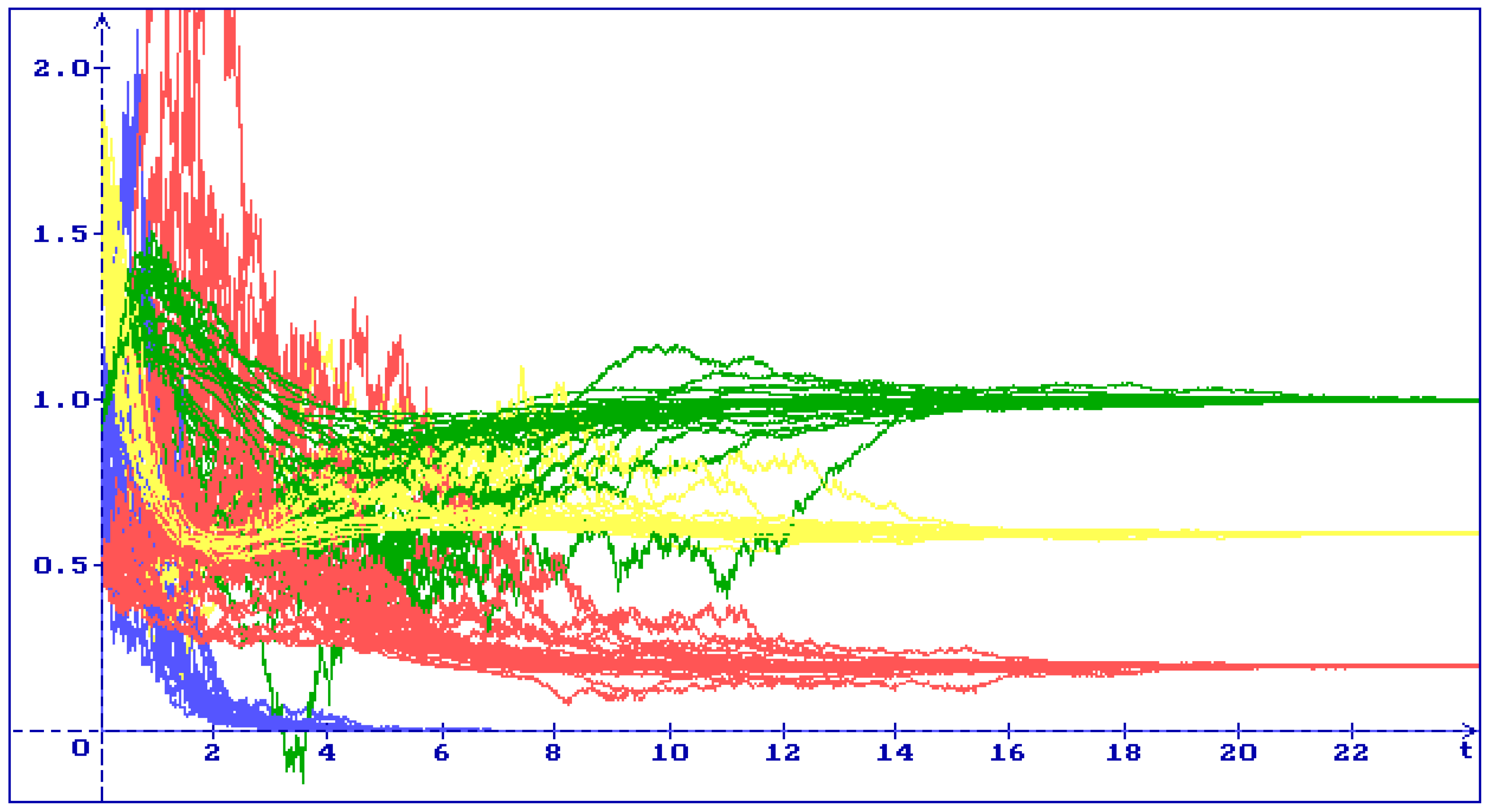
In Figure 2 one can see 30 trajectories of the system (6) solution for the equilibrium E 1 with the initial condition I ( 0 ) = 1.7 , S 1 ( 0 ) = 0.9 , S 2 ( 0 ) = 0.7 , R ( 0 ) = 0.5 : all trajectories I ( t ) (yellow), S 1 ( t ) (green), S 2 ( t ) (blue), R ( t ) (red) converge to the equilibrium E 1 = ( I * , S 1 * , S 2 * , R * ) = ( 1.0769 , 0.2088 , 0 , 0 ) .

4.3. Stability of the Equilibrium E 2 = ( I 2 * , S 12 * , 0 , R 2 * )

For the equilibrium E 2 the system (8) takes the form
z ˙ 0 ( t ) = q ( 1 + λ 1 δ 1 1 ) z 0 ( t ) λ 1 I 2 * z 1 ( t ) λ 2 I 2 * z 2 ( t ) + σ 0 z 0 ( t ) w ˙ 0 ( t ) , z ˙ 1 ( t ) = q λ 1 δ 1 1 z 0 ( t ) ( q + δ 1 R 2 * λ 1 I 2 * ) z 1 ( t ) + α z 2 ( t ) q z 3 ( t ) + σ 1 z 1 ( t ) w ˙ 1 ( t ) , z ˙ 2 ( t ) = ( α + q λ 2 I 2 * + δ 2 R 2 * ) z 2 ( t ) + σ 2 z 2 ( t ) w ˙ 2 ( t ) , z ˙ 3 ( t ) = δ 1 R 2 * z 1 ( t ) + δ 2 R 2 * z 2 ( t ) + σ 3 z 3 ( t ) w ˙ 3 ( t ) ,
where I 2 * and R 2 * are defined in (3).
Lemma 3.
If
p q 2 > 1 λ 1 + 1 δ 1 , 1 + α q > p ( λ 2 δ 1 λ 1 δ 2 ) q 2 ( δ 1 + λ 1 ) + δ 2 δ 1 ,
then the matrix
A = [ q ( 1 + λ 1 δ 1 1 ) λ 1 I 2 * λ 2 I 2 * 0     q λ 1 δ 1 1 0 α q     0 0 ( α + q λ 2 I 2 * + δ 2 R 2 * ) 0     0 δ 1 R 2 * δ 2 R 2 * 0 ]
of the system (26) is the Hurwitz matrix.
Proof. 
The first and the second conditions (27) provide respectively a positivity of R 2 * and a negativity of the coefficient before z 2 ( t ) in the third equation of the system (26). Please note that the inequality
σ 2 2 < 2 q 1 + α q p ( λ 2 δ 1 λ 1 δ 2 ) q 2 ( δ 1 + λ 1 ) δ 2 δ 1
is the necessary and sufficient condition for asymptotic mean square stability of the zero solution of the equation for z 2 ( t ) of the system (26). Therefore, by this condition lim t E z 2 2 ( t ) = 0 it is enough to show that the matrix
A = [ q ( 1 + λ 1 δ 1 1 ) λ 1 I 2 * 0    q λ 1 δ 1 1 0 q     0 δ 1 R 2 * 0 ]
is the Hurwitz matrix. Really, for the matrix (30) we have
T 1 = q ( 1 + λ 1 δ 1 1 ) < 0 , T 2 = q λ 1 2 δ 1 1 I 2 * + q δ 1 R 2 * > 0 , T 3 = q 2 δ 1 R 2 * ( 1 + λ 1 δ 1 1 ) < 0 ,
and
T 1 T 2 = ( q ( 1 + λ 1 δ 1 1 ) ) ( q λ 1 2 δ 1 1 I 2 * + q δ 1 R 2 * ) < q 2 δ 1 R 2 * ( 1 + λ 1 δ 1 1 ) = T 3 .
Therefore, the matrix (30) is the Hurwitz matrix. Therefore the matrix (28) is the Hurwitz matrix too. The proof is completed. □
Corollary 1.
If the conditions (27) and (29) hold then for small enough σ 0 2 , σ 1 2 , σ 3 2 the LMI (12) holds. It means that the zero solution of the linear system (26) is asymptotically mean square stable and therefore (Remark 1) the equilibrium E 2 is stable in probability.
Example 3.
Put
α = 0.4 , λ 1 = 1 , λ 2 = 1.3 , δ 1 = 0.5 , δ 2 = 0.7 , p = 0.9 , q = 0.5 , σ 0 = 0.55 , σ 1 = 0.30 , σ 2 = 0.72 , σ 3 = 0.44 .
By these values of the parameters the conditions (27) and (29) hold:
p q 2 = 3.6 > 1 λ 1 + 1 δ 1 = 3 , 1 + α q = 1.8 > p ( λ 2 δ 1 λ 1 δ 2 ) q 2 ( δ 1 + λ 1 ) + δ 2 δ 1 = 1.28 , σ 2 2 = 0.5184 < 2 q 1 + α q p ( λ 2 δ 1 λ 1 δ 2 ) q 2 ( δ 1 + λ 1 ) δ 2 δ 1 = 0.52 .
Using MATLAB it was shown that by the values of the parameters (31) the matrix (28) satisfies the LMI (12), via Lemma 3 the conditions (13) hold too. Therefore, the equilibrium E 2 is stable in probability.
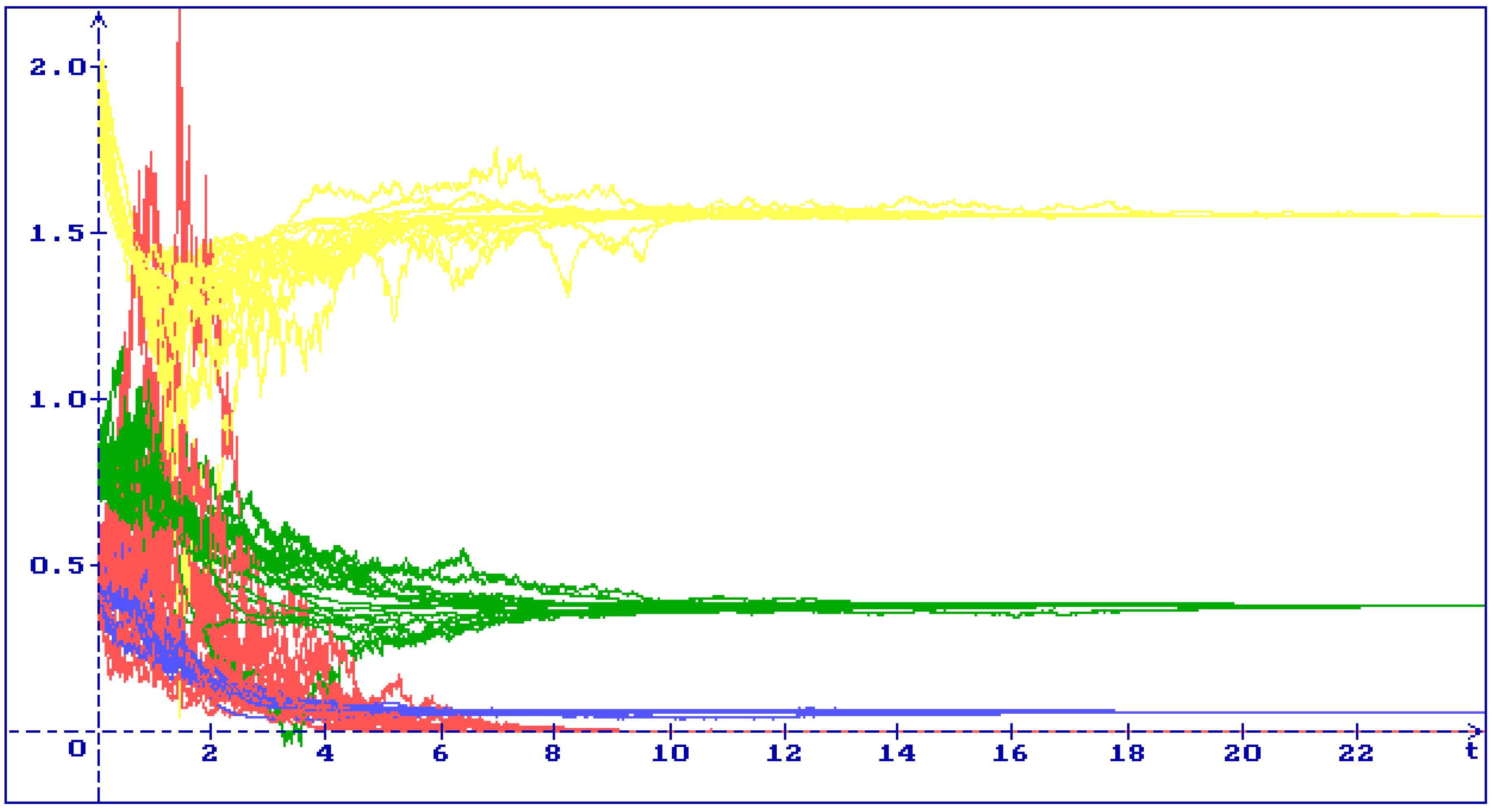
In Figure 3 one can see 30 trajectories of the system (6) solution for the equilibrium E 2 with the initial condition I ( 0 ) = 1.7 , S 1 ( 0 ) = 0.9 , S 2 ( 0 ) = 0.7 , R ( 0 ) = 0.5 : all trajectories I ( t ) (yellow), S 1 ( t ) (green), S 2 ( t ) (blue), R ( t ) (red) converge to the equilibrium E 2 = ( I * , S 1 * , S 2 * , R * ) = ( 0.6 , 1 , 0 , 0.2 ) . In accordance with (5) I * + S 1 * + S 2 * + R * = p q 1 = 1.8 .

4.4. Stability of the Equilibrium E 3 = ( I 3 * , S 13 * , S 23 * , 0 )

For the equilibrium E 3 the system (8) takes the form
z ˙ 0 ( t ) = p λ 2 ( α + q ) 1 z 0 ( t ) λ 1 λ 2 1 ( α + q ) z 1 ( t ) ( α + q ) z 2 ( t ) + σ 0 z 0 ( t ) w ˙ 0 ( t ) , z ˙ 1 ( t ) = λ 1 S 13 * z 0 ( t ) ( q λ 1 λ 2 1 ( α + q ) ) z 1 ( t ) + α z 2 ( t ) δ 1 S 13 * z 3 ( t ) + σ 1 z 1 ( t ) w ˙ 1 ( t ) , z ˙ 2 ( t ) = λ 2 S 23 * z 0 ( t ) δ 2 S 23 * z 3 ( t ) + σ 2 z 2 ( t ) w ˙ 2 ( t ) , z ˙ 3 ( t ) = ( q δ 1 S 13 * δ 2 S 23 * ) z 3 ( t ) + σ 3 z 3 ( t ) w ˙ 3 ( t ) ,
where S 13 * , S 23 * are defined in (3).
Lemma 4.
If
p q 2 > 1 λ 2 1 + α q , 1 λ 1 > 1 λ 2 1 + α q , q > δ 1 S 13 * + δ 2 S 23 * ,
then the matrix
A = [ p λ 2 ( α + q ) 1 λ 1 λ 2 1 ( α + q ) ( α + q ) 0    λ 1 S 13 * ( q λ 1 λ 2 1 ( α + q ) ) α δ 1 S 13 *    λ 2 S 23 * 0 0 δ 2 S 23 *     0 0 0 ( q δ 1 S 13 * δ 2 S 23 * ) ]
of the system (26) is the Hurwitz matrix.
Proof. 
The conditions (33) provide a positivity of S 13 * and S 23 * and a negativity of the diagonal elements of the matrix (34). Please note that the inequality
σ 3 2 < 2 ( q δ 1 S 13 * δ 2 S 23 * )
is the necessary and sufficient condition for asymptotic mean square stability of the zero solution of the equation for z 3 ( t ) of the system (32). Therefore, by this condition lim t E z 3 2 ( t ) = 0 and it is enough to show that the matrix
A = [ p λ 2 ( α + q ) 1 λ 1 λ 2 1 ( α + q ) ( α + q )    λ 1 S 13 * ( q λ 1 λ 2 1 ( α + q ) ) α    λ 2 S 23 * 0 0 ]
with
T 1 = p λ 2 ( α + q ) 1 ( q λ 1 λ 2 1 ( α + q ) ) < 0 , T 2 = p ( α + q ) 1 ( λ 2 q λ 1 ( α + q ) ) + ( α + q ) [ λ 1 2 λ 2 1 S 13 * + λ 2 S 23 * ] > 0 , T 3 = q ( α + q ) ( λ 2 λ 1 ) S 23 * < 0 ,
is the Hurwitz matrix, i.e., T 1 T 2 < T 3 . The proof is completed. □
Corollary 2.
If the conditions (33) and (35) hold then for small enough σ 0 2 , σ 1 2 , σ 2 2 the LMI (12) holds. It means that the zero solution of the linear system (32) is asymptotically mean square stable and therefore (Remark 1) the equilibrium E 3 is stable in probability.
Example 4.
Put
α = 0.8 , λ 1 = 0.3 , λ 2 = 0.9 , δ 1 = 0.8 , δ 2 = 0.7 , p = 1.2 , q = 0.6 , σ 0 = 0.91 , σ 1 = 0.50 , σ 2 = 0.40 , σ 3 = 0.70 .
By these values of the parameters the conditions (33) and (35) hold:
p q 2 = 3.33 > 1 λ 2 1 + α q = 2.59 , 1 λ 1 = 3.33 > 1 λ 2 1 + α q = 2.59 , q = 0.6 > δ 1 S 13 * + δ 2 S 23 * = 0.1715 , σ 3 2 = 0.49 < 2 ( q δ 1 S 13 * δ 2 S 23 * ) = 0.5015 .
Using MATLAB it was shown that by the values of the parameters (37) the matrix (34) satisfies the LMI (12), for the matrix (36) T 1 = 0.9048 < 0 , T 2 = 0.2362 > 0 , T 3 = 0.0320 < 0 , T 3 T 1 T 2 = 0.1817 > 0 , the conditions (13) hold too. Therefore, the equilibrium E 3 is stable in probability.
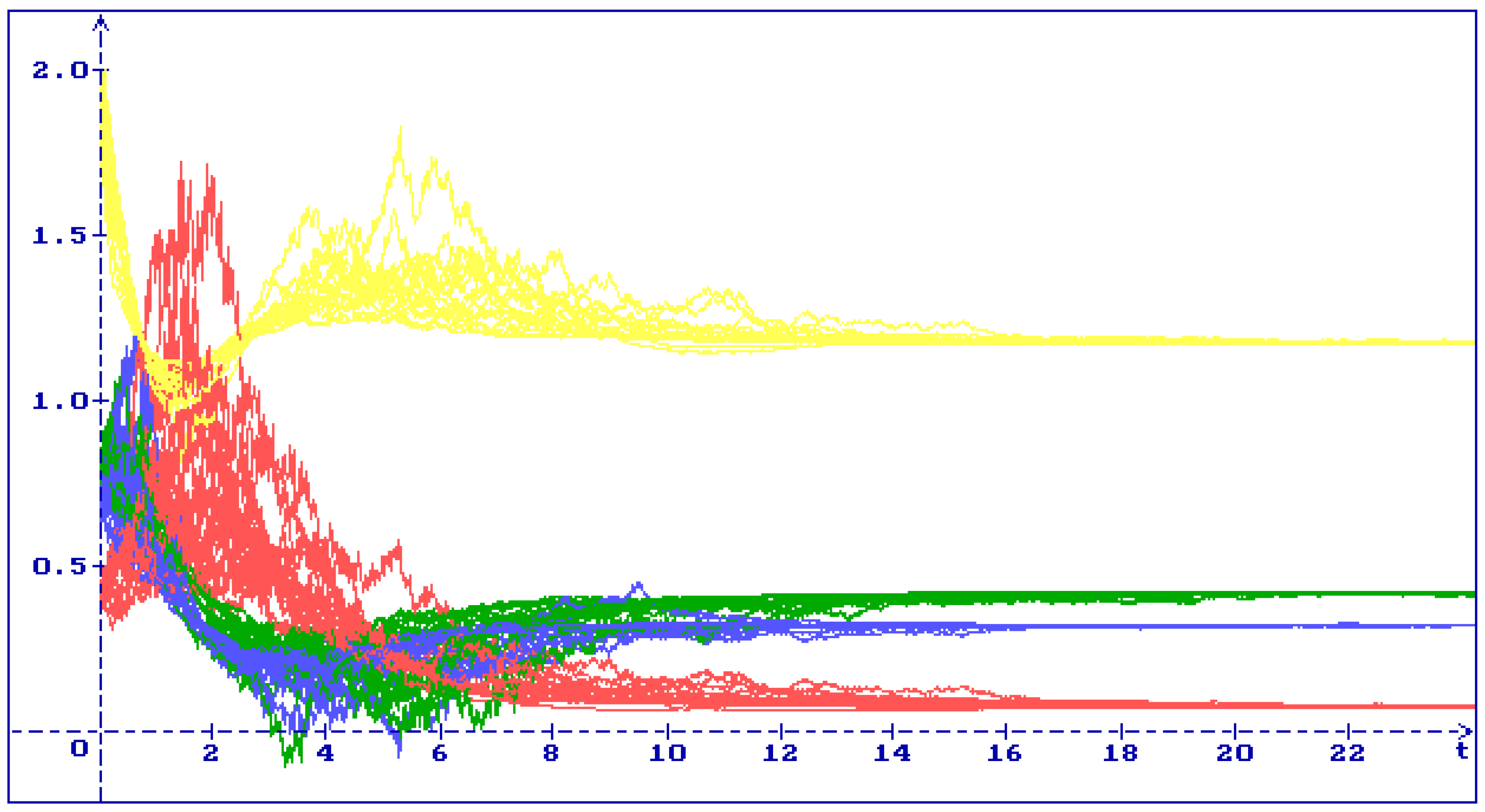
In Figure 4 one can see 30 trajectories of the system (6) solution for the equilibrium E 3 with the initial condition I ( 0 ) = 1.9 , S 1 ( 0 ) = 0.8 , S 2 ( 0 ) = 0.4 , R ( 0 ) = 0.4 : all trajectories I ( t ) (yellow), S 1 ( t ) (green), S 2 ( t ) (blue), R ( t ) (red) converge to the equilibrium E 3 = ( I * , S 1 * , S 2 * , R * ) = ( 1.5556 , 0.3810 , 0.0634 , 0 ) . In accordance with (5) I * + S 1 * + S 2 * + R * = p q 1 = 2 .

4.5. Stability of the Equilibrium E 4 = ( I 4 * , S 14 * , S 24 * , R 4 * )

For the equilibrium E 4 the system (8) by virtue of (2) takes the form
z ˙ 0 ( t ) = p ( I 4 * ) 1 z 0 ( t ) λ 1 I 4 * z 1 ( t ) λ 2 I 4 * z 2 ( t ) + σ 0 z 0 ( t ) w ˙ 0 ( t ) , z ˙ 1 ( t ) = λ 1 S 14 * z 0 ( t ) α S 24 * ( S 14 * ) 1 z 1 ( t ) + α z 2 ( t ) δ 1 S 14 * z 3 ( t ) + σ 1 z 1 ( t ) w ˙ 1 ( t ) , z ˙ 2 ( t ) = λ 2 S 24 * z 0 ( t ) δ 2 S 24 * z 3 ( t ) + σ 2 z 2 ( t ) w ˙ 2 ( t ) , z ˙ 3 ( t ) = δ 1 R 4 * z 1 ( t ) + δ 2 R 4 * z 2 ( t ) + σ 3 z 3 ( t ) w ˙ 3 ( t ) ,
where I 4 * , S 14 * , S 24 * , R 4 * are defined in (3).
Let us show that the matrix
A = [ p ( I 4 * ) 1 λ 1 I 4 * λ 2 I 4 * 0 λ 1 S 14 * α S 24 * ( S 14 * ) 1 α δ 1 S 14 * λ 2 S 24 * 0 0 δ 2 S 24 *    0 δ 1 R 4 * δ 2 R 4 * 0 ]
of the system (38) is the Hurwitz matrix. Really, the conditions (13) for the matrix (39) hold with
T 1 = p ( I 4 * ) 1 α S 24 * ( S 14 * ) 1 < 0 , T 2 = α p S 24 * ( I 4 * S 14 * ) 1 + I 4 * ( λ 1 2 S 14 * + λ 2 2 S 24 * ) + R 4 * ( δ 1 2 S 14 * + δ 2 2 S 24 * ) > 0 , T 3 = α S 24 * ( λ 1 λ 2 I 4 * + δ 1 δ 2 R 4 * ) p ( I 4 * ) 1 R 4 * ( δ 1 2 S 14 * + δ 2 2 S 24 * ) α ( S 24 * ) 2 ( S 14 * ) 1 ( λ 2 2 I 4 * + δ 2 2 R 4 * ) < 0 , T 4 = α p R 4 * ( I 4 * S 14 * ) 1 ( δ 1 2 ( S 14 * ) 2 + δ 2 2 ( S 24 * ) 2 ) + ( λ 2 δ 1 λ 1 δ 2 ) 2 I 4 * S 14 * S 24 * R 4 * > 0 .
Example 5.
Put
α = 0.4 , λ 1 = 0.3 , λ 2 = 0.9 , δ 1 = δ 2 = 0.8 , p = 1.2 , q = 0.6 , σ 0 = 0.51 , σ 1 = 0.51 , σ 2 = 0.55 , σ 3 = 0.34 .
Using MATLAB it was shown that by the values of the parameters (40) the matrix (39) satisfies the LMI (12), the conditions (13) hold too: T 1 = 1.3259 < 0 , T 2 = 0.7020 > 0 , T 3 = 0.1828 < 0 , T 4 = 0.0187 > 0 , T 3 T 1 T 2 = 0.7479 > 0 , ( T 1 T 2 T 3 ) T 3 T 1 2 T 4 = 0.1039 > 0 . Therefore, the equilibrium E 4 is stable in probability.
In Figure 5 one can see 30 trajectories of the system (6) solution for the equilibrium E 4 with the initial condition I ( 0 ) = 1.9 , S 1 ( 0 ) = 0.8 , S 2 ( 0 ) = 0.7 , R ( 0 ) = 0.4 : all trajectories I ( t ) (yellow), S 1 ( t ) (green), S 2 ( t ) (blue), R ( t ) (red) converge to the equilibrium E 4 = ( I * , S 1 * , S 2 * , R * ) = ( 1.1765 , 0.4250 , 0.3250 , 0.0735 ) . In accordance with (5) I * + S 1 * + S 2 * + R * = p q 1 = 2 .
Please note that decreasing δ 2 from δ 2 = 0.8 to δ 2 = 0.7 , we obtain that S 1 * unlike from the previous case is calculated via quadratic equation (see (3)). By that with the same values of all other parameters the equilibrium E 4 a bit changed E 4 = ( I * , S 1 * , S 2 * , R * ) = ( 1.1534 , 0.4543 , 0.3379 , 0.0544 ) , I * + S 1 * + S 2 * + R * = p q 1 = 2 , but remains stable in probability and the conditions (13) hold with T 1 = 1.3379 < 0 , T 2 = 0.6971 > 0 , T 3 = 0.1686 < 0 , T 4 = 0.0143 > 0 , T 3 T 1 T 2 = 0.7641 > 0 , ( T 1 T 2 T 3 ) T 3 T 1 2 T 4 = 0.1033 > 0 .

5. Conclusions

In this paper, it is shown how the dynamics of the very popular I2SR rumor spreading model can be investigated under stochastic perturbations. It is shown that for some equilibria of the considered model it is possible to get conditions for stability in probability in an analytical form, for other equilibria stability condition can be obtained numerically by an appropriate linear matrix inequality via MATLAB.
The proposed way of research can be used for more detail investigation both the considered I2SR rumor spreading model and also all other known type of rumor spreading models [6,7,8,9,10,11,12,13,14,15,16,17,18,19,20,21,22,23,24,25,26,27,28,29].
Besides, this research method can be used for a detailed investigation of many other nonlinear mathematical models (with the order of nonlinearity higher than one) in different other applications. In particular, the proposed method can be used for systems with exponential nonlinearity [34,35], together with stochastic perturbations of the type of white noise other types of perturbations can be used, for instance, perturbations of the type of Poisson’s jumps [35], the method does not depend on the dimension of the considered system and can be used for systems of more than four equations.

Funding

This research received no external funding.

Conflicts of Interest

The author declares no conflict of interest.

Appendix A

Appendix A.1. Equilibria of the System (1)

The equilibria E 0 , , E 3 of the system (1) are obtained from the system (2) quite simply (see (3)). To get the equilibrium E 4 note that from the second and the third equations of the system (2) we obtain
R = 1 δ 1 ( α S 2 S 1 1 q + λ 1 I ) = 1 δ 2 ( λ 2 I ( α + q ) ) .
From this and the first equation of the system (2) we have
I = ( α + q ) δ 1 + ( α S 2 S 1 1 q ) δ 2 λ 2 δ 1 λ 1 δ 2 = p λ 1 S 1 + λ 2 S 2 + q ,
and therefore
( ( α + q ) δ 1 + ( α S 2 S 1 1 q ) δ 2 ) ( λ 1 S 1 + λ 2 S 2 + q ) = p ( λ 2 δ 1 λ 1 δ 2 ) .
From the last equation of the system (2) and R * 0 it follows that
S 2 S 1 1 = 1 δ 2 q S 1 δ 1 .
Substituting (A2) into (A1) we obtain the equation for S 1
( α + q ) δ 1 + α q S 1 δ 1 q δ 2 λ 1 S 1 + λ 2 δ 2 q δ 1 S 1 + q = p ( λ 2 δ 1 λ 1 δ 2 ) , q ( α ( δ 2 δ 1 ) S 1 ) q ( λ 2 + δ 2 ) ( λ 2 δ 1 λ 1 δ 2 ) S 1 = p δ 2 ( λ 2 δ 1 λ 1 δ 2 ) S 1 , q ( δ 2 δ 1 ) ( λ 2 δ 1 λ 1 δ 2 ) S 1 2 [ ( q α + p δ 2 ) ( λ 2 δ 1 λ 1 δ 2 ) + q 2 ( δ 2 δ 1 ) ( λ 2 + δ 2 ) ] S 1 + α q 2 ( λ 2 + δ 2 ) = 0 .
If ( δ 2 δ 1 ) ( λ 2 δ 1 λ 1 δ 2 ) 0 then S 1 is a positive root of the quadratic equation S 1 2 ν 1 S 1 + ν 2 = 0 , where
ν 1 = q α + p δ 2 q ( δ 2 δ 1 ) + q ( λ 2 + δ 2 ) λ 2 δ 1 λ 1 δ 2 , ν 2 = α q ( λ 2 + δ 2 ) ( δ 2 δ 1 ) ( λ 2 δ 1 λ 1 δ 2 ) .
Remark A1.
Please note that a positive root of the quadratic equation S 1 2 ν 1 S 1 + ν 2 = 0 may not exist, for instance, if ν 1 < 0 and ν 2 > 0 . In this case a positive equilibrium E 4 does not exist too. On the other hand for some values of the parameters the quadratic equation S 1 2 ν 1 S 1 + ν 2 = 0 may have two positive roots, for instance, if ν 1 > 0 and 0 < 4 ν 2 < ν 1 2 : S 1 * = 1 2 ( ν 1 ± ν 1 2 4 ν 2 ) . In this case there are two equilibria of the type of E 4 .
If δ 1 = δ 2 = δ , λ 2 > λ 1 then S 1 * = α q 2 ( δ + λ 2 ) δ ( λ 2 λ 1 ) ( q α + p δ ) . If λ 2 δ 1 = λ 1 δ 2 , δ 2 > δ 1 then S 1 * = α δ 2 δ 1 .
If S 1 * is defined then via (2)
S 2 * = 1 δ 2 ( q δ 1 S 1 * ) , I * = p λ 1 S 1 * + λ 2 S 2 * + q , R * = λ 2 I * α q δ 2 .
For positivity of the equilibrium E 4 must be S 1 * < q δ 1 and I * > α + q λ 2 .

Appendix A.2. Stability of the System of Two Stochastic Differential Equations

Consider the system of two stochastic differential equations
x ˙ 1 ( t ) = a 11 x 1 ( t ) + a 12 x 2 ( t ) + σ 1 x 1 ( t ) w ˙ 1 ( t ) , x ˙ 2 ( t ) = a 21 x 1 ( t ) + a 22 x 2 ( t ) + σ 1 x 2 ( t ) w ˙ 2 ( t ) ,
where a i j , σ i , i , j = 1 , 2 , are constants, w 1 ( t ) and w 2 ( t ) are mutually independent standard Wiener processes [30,33].
Lemma A1.
[30] Put A = a i j , i , j = 1 , 2 , A i = det ( A ) + a i i 2 , μ i = 1 2 σ i 2 , i = 1 , 2 , and suppose that the following conditions hold
T r ( A ) = a 11 + a 22 < 0 , det ( A ) = a 11 a 22 a 12 a 21 > 0 , μ 1 < | T r ( A ) | det ( A ) A 2 , μ 2 < | T r ( A ) | det ( A ) A 2 μ 1 A 1 | T r ( A ) | μ 1 .
Then the zero solution of the system (A3) is asymptotically mean square stable.
Remark A2.
Please note that if a 12 a 21 = 0 then the last two conditions in (A4) take the form μ 1 < a 11 , μ 2 < a 22 .

References

  1. Beretta, E.; Kolmanovskii, V.; Shaikhet, L. Stability of epidemic model with time delays influenced by stochastic perturbations. Math. Comput. Simul. 1998, 45, 269–277. [Google Scholar] [CrossRef]
  2. Magal, P.; Webb, G. The parameter identification problem for SIR epidemic models: Identifying unreported cases. J. Math. Biol. 2018, 77, 1629–1648. [Google Scholar] [CrossRef] [PubMed]
  3. Kiouach, D.; Sabbar, Y. Stability and Threshold of a Stochastic SIRS Epidemic Model with Vertical Transmission and Transfer from Infectious to Susceptible Individuals. Discret. Dyn. Nat. Soc. 2018, 2018, 7570296. [Google Scholar] [CrossRef] [Green Version]
  4. Santonja, F.-J.; Shaikhet, L. Analysing social epidemics by delayed stochastic models. Discret. Dyn. Nat. Soc. 2012, 2012, 530472. [Google Scholar] [CrossRef] [Green Version]
  5. Santonja, F.-J.; Shaikhet, L. Probabilistic stability analysis of social obesity epidemic by a delayed stochastic model. Nonlinear Anal. Real World Appl. 2014, 17, 114–125. [Google Scholar] [CrossRef]
  6. Dietz, K. Epidemics and Rumours: A Survey. J. R. Stat. Soc. Ser. A Gener. 1967, 130, 505–528. [Google Scholar] [CrossRef] [Green Version]
  7. Zanette, D.H. Dynamics of rumor propagation on small-world networks. Phys. Rev. E 2002, 65, 041908. [Google Scholar] [CrossRef] [Green Version]
  8. Galam, S. Modelling rumors: The no plane pentagon french hoax case. Physica A 2003, 320, 571–580. [Google Scholar] [CrossRef] [Green Version]
  9. Moreno, Y.; Nekovee, M.; Pacheco, A.F. Dynamics of rumor spreading in complex networks. Phys. Rev. E 2004, 69, 066130. [Google Scholar] [CrossRef] [Green Version]
  10. Nekovee, M.; Moreno, Y.; Bianconi, G.; Marsili, M. Theory of rumour spreading in complex social networks. Physica A 2007, 374, 457–470. [Google Scholar] [CrossRef] [Green Version]
  11. Kawachi, K. Deterministic models for rumor transmission. Nonlinear Anal. Real World Appl. 2008, 9, 1989–2028. [Google Scholar] [CrossRef]
  12. Zhang, Z.; Zhang, Z. An interplay model for rumour spreading and emergency development. Physica A 2009, 388, 4159–4166. [Google Scholar] [CrossRef]
  13. Roshani, F.; Naimi, Y. Effects of degree-biased transmission rate and nonlinear infectivity on rumor spreading in complex social networks. Phys. Rev. E 2012, 85, 036109. [Google Scholar] [CrossRef] [Green Version]
  14. Zhao, L.J.; Wang, J.J.; Chen, Y.C.; Wang, Q.; Cheng, J.J.; Cui, H.X. SIHR rumor spreading model in social networks. Physica A 2012, 391, 2444–2453. [Google Scholar] [CrossRef]
  15. Wang, Y.; Yang, X.; Han, Y.; Wang, X. Rumor spreading model with trust mechanism in complex social networks. Commun. Theor. Phys. 2013, 59, 510–516. [Google Scholar] [CrossRef]
  16. Zhao, L.; Qiu, X.; Wang, X.; Wang, J. Rumor spreading model considering forgetting and remembering mechanisms in homogeneous networks. Physica A 2013, 392, 987–994. [Google Scholar] [CrossRef]
  17. Wang, J.; Zhao, L.; Huang, R. SIRaRu rumor spreading model in complex networks. Physica A 2014, 398, 43–55. [Google Scholar] [CrossRef]
  18. Wang, J.; Zhao, L.; Huang, R. 2SI2R rumor spreading model in homogeneous networks. Physica A 2014, 413, 153–161. [Google Scholar] [CrossRef]
  19. Zan, Y.; Wu, J.; Li, P.; Yu, Q. SICR rumor spreading model in complex networks: Counterattack and self-resistance. Physica A 2014, 405, 159–170. [Google Scholar] [CrossRef]
  20. Ji, K.; Liu, J.; Xiang, G. Anti-rumor dynamics and emergence of the timing threshold on complex network. Physica A 2014, 411, 87–94. [Google Scholar] [CrossRef] [Green Version]
  21. Afassinou, K. Analysis of the impact of education rate on the rumor spreading mechanism. Physica A 2014, 414, 43–52. [Google Scholar] [CrossRef]
  22. Xia, L.L.; Jiang, G.P.; Song, B.; Song, Y.R. Rumor spreading model considering hesitating mechanism in complex social networks. Physica A 2015, 437, 295–303. [Google Scholar] [CrossRef]
  23. Zhang, N.; Huang, H.; Duarte, M.; Zhang, J. Risk analysis for rumor propagation in metropolises based on improved 8-state ICSAR model and dynamic personal activity trajectories. Physica A 2016, 451, 403–419. [Google Scholar] [CrossRef]
  24. Wan, C.; Li, T.; Wang, Y.; Liu, X. Rumor Spreading of a SICS Model on complex social networks with counter mechanism. Open Access Libr. J. 2016, 3, 1–11. [Google Scholar] [CrossRef]
  25. Jie, R.; Qiao, J.; Xu, G.; Meng, Y. A study on the interaction between two rumors in homogeneous complex networks under symmetric conditions. Physica A 2016, 454, 129–142. [Google Scholar] [CrossRef]
  26. Huo, L.; Wang, L.; Song, N.; Ma, C.; He, B. Rumor spreading model considering the activity of spreaders in the homogeneous network. Physica A 2017, 468, 855–865. [Google Scholar] [CrossRef]
  27. Liu, Q.M.; Li, T.; Su, M.C. The analysis of an SEIR rumor propagation model on heterogeneous network. Physica A 2017, 469, 372–380. [Google Scholar] [CrossRef]
  28. Zhu, L.; Wang, Y.G. Rumor spreading model with noise interference in complex social networks. Physica A 2017, 469, 750–760. [Google Scholar] [CrossRef]
  29. Zhang, Y.; Su, Y.; Li, W.; Liu, H. Rumor and authoritative information propagation model considering super spreading in complex social networks. Physica A 2018, 506, 395–411. [Google Scholar] [CrossRef]
  30. Shaikhet, L. Lyapunov Functionals and Stability of Stochastic Functional Differential Equations; Springer Science & Business Media: Berlin, Germany, 2013. [Google Scholar]
  31. Shaikhet, L.; Bunimovich-Mendrazitsky, S. Stability Analysis of Delayed Immune Response BCG Infection in Bladder Cancer Treatment Model by Stochastic Perturbations. Comput. Math. Methods Med. 2018, 2018, 9653873. [Google Scholar] [CrossRef] [PubMed]
  32. Fridman, E.; Shaikhet, L. Simple LMIs for stability of stochastic systems with delay term given by Stieltjes integral or with stabilizing delay. Syst. Control Lett. 2019, 124, 83–91. [Google Scholar] [CrossRef]
  33. Gikhman, I.I.; Skorokhod, A.V. Stochastic Differential Equations; Springer: Berlin/Heidelberg, Germany, 1972. [Google Scholar]
  34. Shaikhet, L. Stability of the zero and positive equilibria of two connected neoclassical growth models under stochastic perturbations. Commun. Nonlinear Sci. Numer. Simul. 2019, 68, 86–93. [Google Scholar] [CrossRef]
  35. Shaikhet, L. Stability of the neoclassical growth model under perturbations of the type of Poisson’s jumps: Analytical and numerical analysis. Commun. Nonlinear Sci. Numer. Simul. 2019, 72, 78–87. [Google Scholar] [CrossRef]
Figure 1. 30 trajectories of the system (6) solution with the initial condition I ( 0 ) = 1.7 , S 1 ( 0 ) = 0.9 , S 2 ( 0 ) = 0.7 , R ( 0 ) = 0.5 : all trajectories I ( t ) (yellow), S 1 ( t ) (green), S 2 ( t ) (blue), R ( t ) (red) converge to the equilibrium E 0 = ( I * , S 1 * , S 2 * , R * ) = ( 1.1429 , 0 , 0 , 0 ) .
Axioms 09 00024 g001
Figure 2. 30 trajectories of the system (6) solution with the initial condition I ( 0 ) = 1.7 , S 1 ( 0 ) = 0.9 , S 2 ( 0 ) = 0.7 , R ( 0 ) = 0.5 : all trajectories I ( t ) (yellow), S 1 ( t ) (green), S 2 ( t ) (blue), R ( t ) (red) converge to the equilibrium E 1 = ( I * , S 1 * , S 2 * , R * ) = ( 1.0769 , 0.2088 , 0 , 0 ) .
Axioms 09 00024 g002
Figure 3. 30 trajectories of the system (6) solution with the initial condition I ( 0 ) = 1.7 , S 1 ( 0 ) = 0.9 , S 2 ( 0 ) = 0.7 , R ( 0 ) = 0.5 : all trajectories I ( t ) (yellow), S 1 ( t ) (green), S 2 ( t ) (blue), R ( t ) (red) converge to the equilibrium E 2 = ( I * , S 1 * , S 2 * , R * ) = ( 0.6 , 1 , 0 , 0.2 ) .
Axioms 09 00024 g003
Figure 4. 30 trajectories of the system (6) solution with the initial condition I ( 0 ) = 1.9 , S 1 ( 0 ) = 0.8 , S 2 ( 0 ) = 0.4 , R ( 0 ) = 0.4 : all trajectories I ( t ) (yellow), S 1 ( t ) (green), S 2 ( t ) (blue), R ( t ) (red) converge to the equilibrium E 3 = ( I * , S 1 * , S 2 * , R * ) = ( 1.5556 , 0.3810 , 0.0634 , 0 ) .
Axioms 09 00024 g004
Figure 5. 30 trajectories of the system (6) solution with the initial condition I ( 0 ) = 1.9 , S 1 ( 0 ) = 0.8 , S 2 ( 0 ) = 0.7 , R ( 0 ) = 0.4 : all trajectories I ( t ) (yellow), S 1 ( t ) (green), S 2 ( t ) (blue), R ( t ) (red) converge to the equilibrium E 4 = ( I * , S 1 * , S 2 * , R * ) = ( 1.1765 , 0.4250 , 0.3250 , 0.0735 ) .
Axioms 09 00024 g005