2.2. Background
In this article, we show how to define a metric on
(see Introduction). For any Cantorian set
S, we use
to denote the cardinality of
S. Let
d be an arbitrary metric on
satisfying
for all
. Observe that
d is a metric (for our generalization purpose) on
, which lays a foundation for our latter definition of a metric on
. Let
be arbitrary. Let
denote the set of all the functions from
A to
B, in which the repeated elements are deemed distinct.
Example 1. Suppose and , and . Then, . For clarity, one could simply associate A and B with their ranked multiplicities as follows: and and ρ could also be represented by . To save space, we simply use for the representation in this article.
For any function , we use and to denote its domain and codomain, respectively. For the previous example, and . We use to denote the image , in particular to denote the image of and to denote the pre-image of S. If , we use to denote whose domain is restricted to S. One candidate in mind is .
Definition 8. (Bijective embeddings) Define Example 2. Suppose ρ is defined in Example 1. Since , by the above definition, one has . On the other hand, suppose , then , since . Note that . Moreover, if , then ; similarly, if , then . Take A and B in Example 1 for example. One has .
Definition 9. For any function , we call it a a matched function. We call a matched pair. Every remaining element in is called a mismatched element.
On this basis, we could define the distance for the matched elements and the distance for the mismatched elements as follows:
Definition 10. For any , definewhere and and denote the domain and codomain of φ, respectively. represents the distance of all the matched elements (or the sum of the distances of all the matched pairs), while represents the distance of all the mismatched elements in the range. iff . For example, if and is defined by , then the matched part yields , where denotes the th repetition of i and the mismatched part . Next, we define the set of all minimal distances consisting of the matched parts and the mismatched parts. Definition 11. (Minimal matched functions) Define Definition 12. (Distance function) Define by By the definition, one has
for any
. In the following, we show that
is indeed a metric. The reasoning will be proceeded by their relations (i.e., larger, less than and equal to) between cardinalities of
, and
C, i.e.,
, and
. To validate that
is a metric, we need to consider all the 27 relations between
and
: for example,
. In order to facilitate our computing, we encode the 27 relations by the following set
in which each
represents the relation
and
, respectively, where
, and 3 represent the relation
and > correspondingly. For example,
represents the relation
, and
. By the transitivity of their cardinalities, only 13 of the 27 relations are valid (shown in Lemma 1). Moreover, these 13 relations could be further reduced to 8 relations by the symmetry of
, i.e.,
as shown in Corollary 1. If
is a bijective function, we use
to denote its inverse function. In the following, let
, and
be arbitrary. Before we proceed further, we have the definitions:
We use to denote , if and to denote , if .
We use to denote , if and to denote , if .
We use to denote , if and to denote , if .
Though there are 27 relations between the cardinalities of , and C, only 13 of them are valid as shown in the following lemma.
Lemma 1. There are only 13 relations which do not violate the transitivity property in terms of their cardinalities: Proof. The result follows immediately from their relations. Take the relation for example. Recall that represents the relation , in which the property of transitivity holds. One could verify that each of the other 12 relations also holds the transitivity property. However, the other 15 relations fail the transitivity property: for example ( i.e., ). ☐
Lemma 2. (Non-negative, symmetric)
.
iff .
.
Proof. The first statement follows immediately from the definition and the third one follows from the fact that . Here we show the second one. Suppose , then , where I is the identity function. Suppose . Then, there are two cases: either or . For the former one, one has , i.e., . For the latter one, one has and thus , i.e., . Hence, we have shown iff . ☐
In the following, we show the triangle inequality of . Let us show the following corollary first.
Corollary 1. To show δ satisfy the triangle inequality, it suffices to consider the following eight relations: Proof. By Equation (
7) and Lemma 1,
A and
C are interchangeable, i.e., the relations
are equivalent to (respectively)
☐
By this corollary, we only need to consider the triangle inequality of the above-mentioned eight relations.
Lemma 3. If , then .
Proof. Since
, it follows
and
Since
, by the definition of
d, it follows
i.e.,
. ☐
Lemma 4. If , then .
Proof. By the definition
, it follows
where
denotes
. Furthermore,
Henceforth, by the properties of
d and the definition of
☐
Lemma 5. If , then .
Proof. By the definition
, it follows
Henceforth, by the triangle inequality of
d ☐
Lemma 6. If , then .
Proof. By the triangle inequality of
d and the definitions of
☐
Lemma 7. If , then .
Proof. By the definitions,
where
denotes
. Moreover,
Hence, by the triangle inequality of
d and the definitions of
☐
Lemma 8. If , then .
Proof. By the definitions of
where
denotes
;
Then, by the triangle inequality of
d and the definitions of
☐
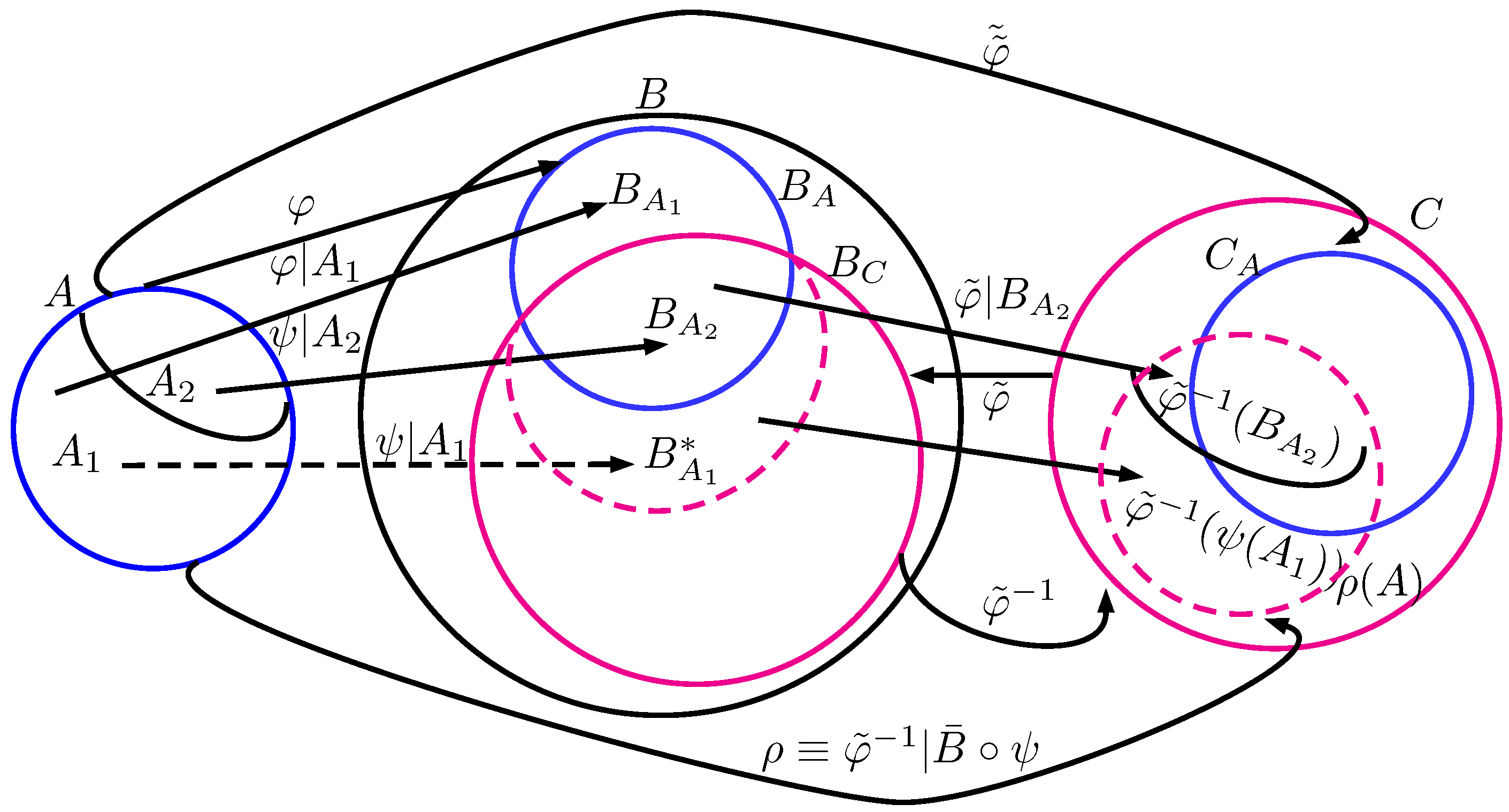
Lemma 9. If , then .
Proof. We derive the three components one by one. Firstly, suppose
is a function satisfying
(as shown in
Figure 1), i.e.,
for all
. By the definitions of
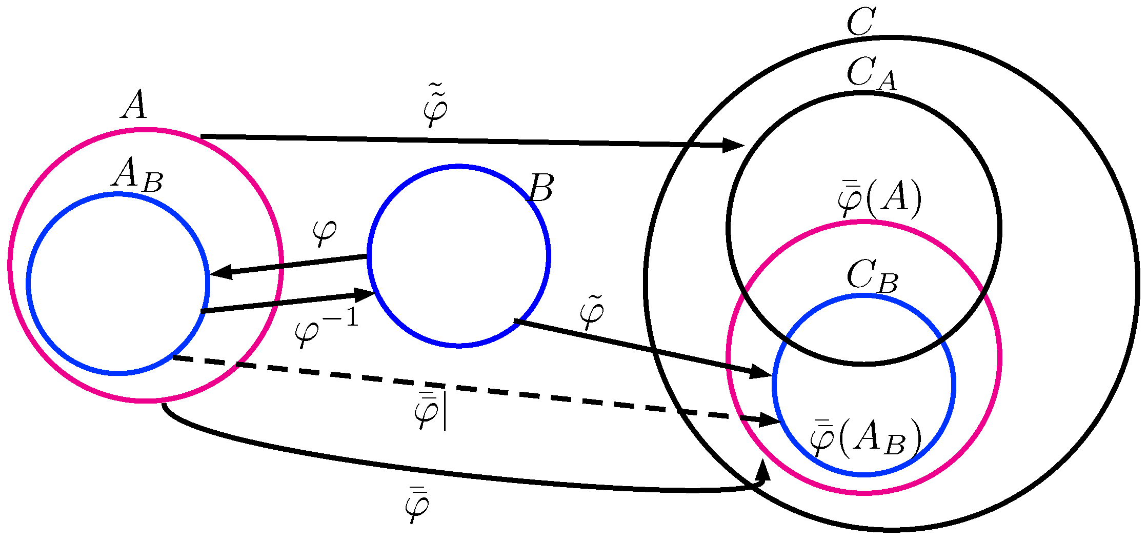
Lemma 10. If , then .
Proof. Suppose
. Suppose
. Suppose
Choose a function
, in which
, i.e.,
. Suppose
, where
. Let
denote the composition
(or simply
). Then,
and
as shown in
Figure 2. Furthermore, by the definition of
,
Henceforth, by Equations (
3)–(
5), it follows
☐
Theorem 1. is a metric space.
Proof. By Lemmas 2–10 and Corollary 1, the result follows immediately. ☐


