A Gradient System for Low Rank Matrix Completion

Abstract

In this article we present and discuss a two step methodology to find the closest low rank completion of a sparse large matrix. Given a large sparse matrix M, the method consists of fixing the rank to r and then looking for the closest rank-r matrix X to M, where the distance is measured in the Frobenius norm. A key element in the solution of this matrix nearness problem consists of the use of a constrained gradient system of matrix differential equations. The obtained results, compared to those obtained by different approaches show that the method has a correct behaviour and is competitive with the ones available in the literature.

1. Introduction

A large class of datasets are naturally stored in matrix form. In many important applications, the challenge of filling a matrix from a sampling of its entries can arise; this is known as the matrix completion problem. Clearly, such a problem needs some additional constraints to be well-posed. One of its most interesting variants is to find the lower rank matrices that best fit the given data. This constrained optimization problem is known as low-rank matrix completion.

Let $M\in {\mathbb{R}}^{m\times n}$ be a matrix that is only known on a subset, $\Omega$, of its entries. In [1], the authors provided conditions on the sampling of observed entries, such that the problem which arises has a high probability of not being undetermined. The classical mathematical formulation for the low rank matrix completion problem is :

$$\begin{array}{c}\hfill minrank\left(X\right)\\ \hfill s.t.P_{\Omega }\left(X\right)=P_{\Omega }\left(M\right)\end{array}$$

where $P_{\Omega }$ is the projection onto $\Omega$ defined as a function

$$P_{\Omega }:{\mathbb{R}}^{m\times n}⟶{\mathbb{R}}^{m\times n}$$

such that

$$X_{i,j}⟼\left\{\begin{array}{c}{X}_{i,j}if(i,j)\in \Omega \hfill \\ 0if(i,j)\notin \Omega \hfill \end{array}\right.$$

This approach may seem like the most natural to describe the problem, but it is not very useful in practice, since it is well known to be NP-hard [2]. In [3], the authors stated the problem as

$$\begin{array}{c}\hfill {min\left|\right|X\left|\right|}_{\ast }\\ \hfill s.t.P_{\Omega }\left(X\right)=P_{\Omega }\left(M\right)\end{array}$$

where ${\left|\right|\left|\right|}_{\ast }$ is the nuclear norm of the matrix, which is the sum of its singular values. This is a convex optimization problem and the authors proved that when $\Omega$ is sampled uniformly at random and is sufficiently large, the previous relaxation can recover any matrix of rank r with high probability. We will consider the following formulation as in [4,5],

$$\begin{array}{c}\hfill min\frac{1}{2}\left|\right|P_{\Omega }\left(X\right)-P_{\Omega }\left(M\right){\left|\right|}_F^2\\ \hfill s.t.rank\left(X\right)=r\end{array}$$

Notice that, the projection $P_{\Omega }\left(X\right)$ can be written as a Hadamard product. If we identify the subset $\Omega$ of the fixed entries with the matrix $\Omega$ such that

$${\Omega }_{i,j}=\left\{\begin{array}{c}1if(i,j)\in \Omega \hfill \\ 0if(i,j)\notin \Omega \hfill \end{array}\right.$$

it is clear that $P_{\Omega }\left(X\right)=\Omega \circ X$. By considering the manifold

$${\mathcal{M}}_r=\{X\in {\mathbb{R}}^{n\times m}:rank\left(X\right)=r\}$$

we can write the problem as

$$\underset{X\in {\mathcal{M}}_r}{min}\frac{1}{2}\left|\right|\Omega \circ {(X-M)\left|\right|}_F^2$$

(1)

This approach is based on the assumption of knowing in advance the rank r of the target matrix. A key feature of the problem is that $r\ll min\{m,n\}$, that translates, from a practical point of view in a small increase of the cost to eventually update r. In [6] is well explained the possibility of estimating the rank (unknown a priori) based on the gap between singular values of the “trimmed” partial target matrix M. Furthermore, the authors highlight that in collaborative filtering applications, r ranged between 10 and 30. In [4], the author employed optimization techniques widely exploiting the structure of smooth Riemaniann manifold of ${\mathcal{M}}_r$. The same tools are used in [5], where the authors considered the matrix completion in the presence of outliers. In the recent work [7], the authors provide a non convex relaxation approach for matrix completion in presence of non Gaussian noise and or outliers, by employing the correntropy induced losses. In [8], the authors survey on the literature on matrix completions and deal with target matrices, whose entries are affected by a small amount of noise. Recently, the problem became popular thanks to collaborative filtering applications [9,10] and the Netflix problem [11]. It can also be employed in other fields of practical applications such as sensor network localization [12], signal processing [13] and reconstruction of damaged images [14]. A very suggestive use of modeling as low rank matrix completion problem has been done in biomathmatics area, as shown in [15] for gene-disease associations. Applications to minimal representation of discrete systems can be considered as of more mathematical feature [16]. What makes the problem interesting are not just the multiple applications, but also its variants, such as, for example, structured [17] and Euclidean distance matrix cases [18]. In this paper a numerical technique to solve the low rank matrix completion problem is provided, which makes use of a gradient system of matrix ODEs.

2. General Idea : Two-Level Method

Let us write the unknown matrix X of the problem (1) as $X=\epsilon E$ with $\epsilon >0$ and ${\left|\right|E\left|\right|}_F=1$. For a fixed norm $\epsilon >0$, we aim to minimize the functional

$$F_{\epsilon }\left(E\right):=\left|\right|\Omega \circ {(\epsilon E-M)\left|\right|}_F^2$$

(2)

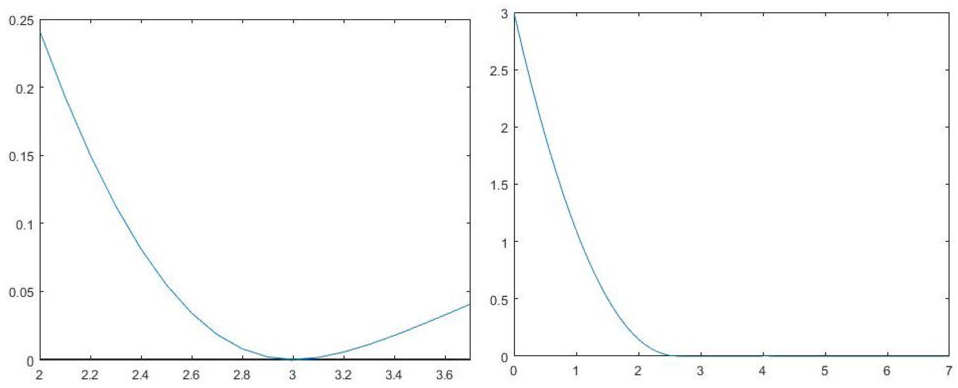
constrained by $E\in {\mathcal{M}}_r$ and ${\left|\right|E\left|\right|}_F=1$ (see [19]). By computing the stationary point of a suitable differential equation, we will find a local minimum $E_{\epsilon }$ of the functional. Setting $f\left(\epsilon \right)=F_{\epsilon }\left(E_{\epsilon }\right)$, we will look for the minimum value of $\epsilon$, say ${\epsilon }_{\ast }$, such that $f\left({\epsilon }^{\ast }\right)=0$, by using a Newton-like method. The behaviour of $f\left(\epsilon \right)$ in a left neighbourhood of ${\epsilon }^{\ast }$ is well understood. For $\epsilon \ge {\epsilon }^{\ast }$ it is more challenging. We discuss two possible scenarios; ${\epsilon }^{\ast }$ can be a strict local minimum point or $f\left(\epsilon \right)$ can become identically zero when $\epsilon$ exceeds ${\epsilon }^{\ast }$. The two situations depend on the rank constraint and on the sparsity pattern. To motivate our assumption, we now present two simple illustrative examples. Suppose that we aim to recover the matrix

$$M=\left(\begin{array}{ccc}1& 1& \ast \\ 1& \ast & 1\\ 1& \ast \end{array}\right).$$

If we constrain the problem by imposing that the rank of the solution has to be equal to 1, we have a strict point of minimum for ${\epsilon }^{\ast }=3$ and the optimal rank-1 matrixthat fits perfectly the given entries of M is

$$S=\left(\begin{array}{ccc}1& 1& 1\\ 1& 1& 1\\ 1& 1& 1\end{array}\right).$$

If we consider the problem of recovering the matrix

$$Y=\left(\begin{array}{ccc}1& 1& 1\\ 1& \ast & 1\\ \ast & 1\end{array}\right)$$

requiring that the solution has to be of rank 2, we have that the solutions of minimal norm ${\epsilon }^{\ast }=2.6458$ are

$$X_1=\left(\begin{array}{ccc}1& 1& 1\\ 1& 1& 1\\ 0& 0& 1\end{array}\right),X_2=\left(\begin{array}{ccc}1& 1& 1\\ 1& 0& 1\\ 1& 0& 1\end{array}\right)$$

However, for all $\epsilon >{\epsilon }^{\ast }$, we have a point of minimum of $f\left(\epsilon \right)$. To understand this behaviour, we can intuitively think that there are a lot of “possibilities” to realize a rank-2 matrix “filling” the unknown entries of Y. For example,

$$X_1(\alpha ,\beta )={\left\{\left(\begin{array}{ccc}1& 1& 1\\ 1& 1& 1\\ \alpha & \beta & 1\end{array}\right)\right\}}_{\alpha ,\beta \in \mathbb{R},\alpha \ne 1\vee \beta \ne 1},X_1(\alpha ,\beta )={\left\{\left(\begin{array}{ccc}1& 1& 1\\ 1& \alpha & 1\\ 1& \beta & 1\end{array}\right)\right\}}_{\alpha ,\beta \in \mathbb{R},\alpha \ne 1\vee \beta \ne 1}$$

are families of solutions of the problem.In the Figure 1, we show the graphics of $f\left(\epsilon \right)$ for the two problems considered.

The paper is structured as follows. In Section 3 and Section 5 we discuss the two level method designed to solve the problem (1). A characterization of local extremizers for the functional (2) is given in Section 4. In Section 6 we present a suitable splitting method for rank-r matricial ODEs employed in the context of the inner iteration. Finally, numerical experiments are showed in Section 7.

3. Differential Equation for E

3.1. Minimizing $F_{\epsilon }\left(E\right)$ for Fixed $\epsilon$

Suppose that $E\left(t\right)$ is a smooth matrix valued function of t. (We omit the argument t of $E\left(t\right)$). Our goal is to find an optimal direction $\dot{E}=Z$ (see [19,20]) such that the functional (2) is characterized by the maximal local decrease, in a way that the matrix E remains in the manifold ${\mathcal{M}}_r$ .

To deal with this goal, we differentiate (2) with respect to t

$$\begin{array}{c}\hfill {\displaystyle \frac{d}{dt}}{F}_{\epsilon }\left(E\right)={\displaystyle \frac{d}{dt}}\frac{1}{2}\left|\right|\Omega \circ {(\epsilon E-M)\left|\right|}_F^2=\frac{1}{2}{\displaystyle \frac{d}{dt}}〈\Omega \circ (\epsilon E-M),\Omega \circ (\epsilon E-M)〉=\epsilon \langle \Omega \circ \dot{E},\Omega \circ (\epsilon E-M)\rangle \end{array}$$

Setting

$$G:=\Omega \circ (\epsilon E-M)$$

(3)

and since by definition of $\Omega$, $\Omega \circ \Omega =\Omega$, it is clear that $\Omega \circ G=G$.

Thus, we have

$$\begin{array}{c}\hfill \langle \Omega \circ \dot{E},\Omega \circ G\rangle =\langle \Omega \circ \dot{E},G\rangle =\sum _{i,j}{\Omega }_{ij}{\dot{E}}_{ij}{G}_{ij}=\sum _{i,j}{\dot{E}}_{ij}{\Omega }_{ij}{G}_{ij}=\langle \dot{E},\Omega \circ G\rangle =\langle \dot{E},G\rangle \end{array}$$

Hence, we have

$${\displaystyle \frac{d}{dt}}{F}_{\epsilon }\left(E\left(t\right)\right)=\epsilon \langle \dot{E},G\rangle$$

(4)

which identifies G as the free gradient of the functional. We have now to include the constraint ${\left|\right|E\left|\right|}_F^2=1$. By differentiation

$${\displaystyle \frac{d}{dt}}{\left|\right|E\left|\right|}_F^2=0\Rightarrow \langle E,\dot{E}\rangle =0$$

we gain a linear constraint for $\dot{E}$. By virtue of the rank constraint in (5), we must guarantee that the motion of E remains in the manifold ${\mathcal{M}}_r$ for all t. In order to get it, we require the derivative $\dot{E}$ to lie in the tangent space in E to ${\mathcal{M}}_r$, for all t. These considerations led us to the following optimization problem.

$$Z_{\ast }=\underset{{\left|\right|Z\left|\right|}_F=1,\langle E,Z\rangle =0,Z\in {\mathcal{T}}_E{\mathcal{M}}_r}{arg\; min}\langle Z,G\rangle$$

(5)

where ${\mathcal{T}}_E{\mathcal{M}}_r$ denotes the tangent space to ${\mathcal{M}}_r$ at E. The constraint ${\left|\right|Z\left|\right|}_F=1$ is simply introduced to get a unique direction Z. In the following, we will denote by $P_E(·)$ the orthogonal projection on ${\mathcal{T}}_E{\mathcal{M}}_r$.

3.2. Rank-r Matrices and Their Tangent Matrices

See [21]. Every real rank-r matrix E of dimension $n\times m$ can be written in the form

$$E=US{V}^T$$

(6)

where $U\in {\mathbb{R}}^{n\times r}$ and $V\in {\mathbb{R}}^{m\times r}$ have orthonormal columns, i.e.,

$$U^{T}U=I_r,V^{T}V=I_r$$

and nonsingular $S\in {\mathbb{R}}^{r\times r}$. In particular, when S is diagonal, we find the SVD. The decomposition (6) is not unique; simply replacing U by $\overline{U}=UP$ and V by $\widehat{V}=VQ$ with orthogonal matrices $P,Q\in {\mathbb{R}}^{r\times r}$ and S by $\widehat{S}=P^{T}SQ$, we get the same matrix $E=US{V}^T=\widehat{U}\widehat{S}{\widehat{V}}^T$. However, we can make the decomposition unique in the tangent space. For all E in the manifold ${\mathcal{M}}_r$, let us consider the tangent space ${\mathcal{T}}_E{\mathcal{M}}_r$. It is a linear space and every tangent matrix is of the form

$$\dot{E}=\dot{U}S{V}^T+U\dot{S}{V}^T+US{\dot{V}}^T$$

where $\dot{S}\in {\mathbb{R}}^{r\times r}$, $U^T\dot{U}$ and $V^T\dot{V}$ are skew-symmetric $r\times r$ matrices. $\dot{S},\dot{U},\dot{V}$ are uniquely determined by $\dot{E}$ and $U,V,S$ by imposing the gauge conditions

$$U^T\dot{U}=0,V^T\dot{V}=0$$

We consider the following important result from [21], thanks to which it is possible to obtain a formula for the projection of a matrix onto the tangent space to a rank-r matrices.

Lemma 1.

The orthogonal projection onto the tangent space ${\mathcal{T}}_E{\mathcal{M}}_r$ at $E=US{V}^T\in {\mathcal{M}}_r$ is given by

$$P_E\left(Z\right)=Z-(I-U{U}^T)Z(I-V{V}^T)$$

for $Z\in {\mathbb{R}}^{n\times m}$.

3.3. Steepest Descent Dynamics

Lemma 2.

Let $E\in {\mathbb{R}}^{n\times m}$ be a real matrix of unit Frobenius norm, such that it is not proportional to $P_E\left(G\right)$. Then, the solution of (5) is given by

$$\mu Z_{\ast }=-P_E\left(G\right)+\langle E,P_E\left(G\right)\rangle E$$

(7)

where μ is the reciprocal of the Frobenius norm on the right-hand side.

Proof. 

Let be $E_{\perp }=\{Z\in {\mathbb{R}}^{n\times m}:\langle E,Z\rangle =0\}$. The function $\langle Z,G\rangle$ is an inner product and the feasible region $\mathcal{R}=E_{\perp }\cap {\mathcal{T}}_E{\mathcal{M}}_r$ is a linear subspace, since it is intersection of subspaces. By observing that the inner product with a given vector is minimized over a subspace by orthogonally projecting the vector onto the subspace, we can say that the solution of (5) is a matrix proportional to the normalized orthogonal projection of the free gradient G onto $\mathcal{R}$. Therefore,

$$P_{\mathcal{R}}\left(G\right)=P_{E^{\perp }}\left(P_E\left(G\right)\right)=P_E\left(G\right)-{\displaystyle \frac{\langle E,P_E\left(G\right)\rangle }{\langle E,E\rangle }}{P}_E\left(G\right)$$

Note that $P_{\mathcal{R}}\left(G\right)=P_{E^{\perp }}\left(P_E\left(G\right)\right)$, since $P_{E^{\perp }}$ and $P_E$ commute. Since ${\left|\right|E\left|\right|}_F=1$, we have that the solution is given by (7). ☐

The Expression (4), jointly with the Lemma 2 suggest to consider the following gradient system for $F_{\epsilon }\left(E\right)$

$$\dot{E}=-P_E\left(G\right)+\langle E,P_E\left(G\right)\rangle E$$

(8)

To get the differential equation in a form involving the factors in $E=US{V}^T$, we use the following result.

Lemma 3

(See [21]). For $E=US{V}^T\in {\mathcal{M}}_r$, with nonsingular $S\in {\mathbb{R}}^{r\times r}$ and with $U\in {\mathbb{R}}^{n\times r}$ and ${\mathbb{R}}^{n\times r}$ having orthonormal columns, the equation $\dot{E}=P_E\left(Z\right)$ is equivalent to $\dot{E}=\dot{U}S{V}^T+U\dot{S}{V}^T+US{\dot{V}}^T$, where

$$\left\{\begin{array}{c}\dot{S}=U^{T}ZV,\hfill \\ \dot{U}=(I-U{U}^T)ZV{S}^{-1},\hfill \\ \dot{V}=(I-V{V}^T)Z^{T}V{S}^{-T}\hfill \end{array}\right.$$

In our case $Z=-P_E\left(G\right)+\langle E,P_E\left(G\right)\rangle E$, this yields that the differential Equation (8) for $E=US{V}^T$ is equivalent to the following system of differential equations for $S,V,U$,

$$\left\{\begin{array}{c}\dot{S}=U^T(-P_E\left(G\right)+\langle E,P_E\left(G\right)\rangle E)V,\hfill \\ \dot{U}=(I-U{U}^T)(-P_E\left(G\right)+\langle E,P_E\left(G\right)\rangle E)V{S}^{-1},\hfill \\ \dot{V}=(I-V{V}^T){(-P_E\left(G\right)+\langle E,P_E\left(G\right)\rangle E)}^{T}V{S}^{-T}\hfill \end{array}\right.$$

(9)

The following monotonicity result is an immediate consequence of the fact that the differential equation is the gradient flow for $F_{ϵ}$ on the manifold of matrices, of fixed rank r, and unit norm.

Theorem 1.

Let be $E\left(t\right)\in {\mathcal{M}}_r$ a solution of unit Frobenius norm of the matrix differential Equation (8). Then

$$\frac{d}{dt}{F}_{\epsilon }\left(E\left(t\right)\right)\le 0$$

Proof. 

By Cauchy-Schwarz inequality,

$$\begin{array}{c}\hfill |\langle E,P_E\left(G\right)\rangle {|\le |\left|E\right||}_F\left|\right|P_E{\left(G\right)\left|\right|}_F=\left|\right|P_E\left(G\right){\left|\right|}_F\end{array}$$

Therefore, using (8),

$$\begin{array}{cc}\hfill \frac{d}{dt}{F}_{\epsilon }\left(E\left(t\right)\right)=\epsilon \langle \dot{E},G\rangle & =\epsilon \langle -P_E\left(G\right)+\langle E,\langle P_E\left(G\right)\rangle E,G\rangle =\epsilon \left(-\langle P_E\left(G\right),G\rangle +\langle E,P_E\left(G\right)\rangle \langle E,G\rangle \right)=\hfill \\ & \hfill \epsilon \left(-\langle P_E\left(G\right),P_E\left(G\right)\rangle +{\langle E,P_E\left(G\right)\rangle }^2\right)=\epsilon \left(-\left|\right|P_E\left(G\right){\left|\right|}_F^2+\langle E,P_E\left(G\right)\rangle \right)\le 0\end{array}$$

 ☐

4. Stationary points

Since we are interested to minimize $F_{\epsilon }\left(E\right)$, we focus on the equilibria of (8), which represents local minima of (2).

Lemma 4.

The following statements are equivalent along the solutions of (8):

(a) 

${\displaystyle \frac{d}{dt}}{F}_{\epsilon }\left(E\right)=0$.

(b) 

$\dot{E}=0$.

(c) 

E is a real multiple of $P_E\left(G\right)$.

Proof. 

From the expression (4), clearly (b) implies (a).

Supposing (c), we can write $P_E\left(G\right)=\alpha E$ with $\alpha \in \mathbb{R}$ and by substitution in (8) we get

$$\dot{E}=-\alpha E+\langle E,\alpha E\rangle E=\alpha \left(-E+{\left|\right|E\left|\right|}_{F}E\right)=\alpha \left(-E+E\right)=0$$

that is (b). So, it remains to show that (a) implies (c).

Note that:

$$\begin{array}{c}\hfill {\displaystyle \frac{d}{dt}}{F}_{\epsilon }\left(E\left(t\right)\right)=\epsilon \langle \dot{E},G\rangle =\epsilon \langle -P_E\left(G\right)+\langle E,P_E\left(G\right)\rangle E,G\rangle \\ \hfill =\epsilon \langle -P_E\left(G\right),G\rangle +\langle E,P_E\left(G\right)\rangle \langle E,G\rangle =\epsilon \left(-\left|\right|P_E\left(G\right){\left|\right|}_F^2+{\langle E,P_E\left(G\right)\rangle }^2\right)\end{array}$$

So, since $\epsilon >0$, we have

$${\displaystyle \frac{d}{dt}}{F}_{\epsilon }\left(E\left(t\right)\right)=0⟺-\left|\right|P_E\left(G\right){\left|\right|}_F^2+{\langle E,P_E\left(G\right)\rangle }^2=0$$

the last equality holds only if $E=\alpha P_E\left(G\right)$ for $\alpha \in \mathbb{R}$, that is (c). ☐

The following result characterizes the local extremizers.

Theorem 2.

Let $E_{\ast }\in {\mathcal{M}}_r$ be a real matrix of unit Frobenius norm. Then, the following two statements are equivalent:

(a) 

Every differentiable path $E\left(t\right)\in {\mathcal{M}}_r$ (for small $t\ge 0$ ) with ${\left|\right|E\left|\right|}_F=1$ and $E\left(0\right)=E_{\ast }$ satisfies

$${\displaystyle \frac{d}{dt}}{F}_{\epsilon }\left(E\left(t\right)\right)\ge 0$$

(b) 

There exists a $\gamma >0$ such that

$$E_{\ast }=-\gamma P_E\left(G\right)$$

Proof. 

The strategy of the proof is similar to [22]. Assume that (a) does not hold. Then, there exists a path $E\left(t\right)\in {\mathcal{M}}_r$ through $E_{\ast }$ such that ${\displaystyle \frac{d}{dt}}{F}_{\epsilon }\left(E\left(t\right)\right){\mid }_{t=0}<0$. Thus, Lemma 2 shows that also the solution path of (8) passing through $E_{\ast }$ is such a path. So $E_{\ast }$ is not a stationary point of (8), and according to the Lemma 4, it is not a real multiple of $P_E\left(G\right)$.

If $E_{\ast }$ is not a multiple of $P_E\left(G\right)$, then $E_{\ast }$ is not a stationary point of (8) and Theorem 1 and Lemma 4 ensure that ${\displaystyle \frac{d}{dt}}{F}_{\epsilon }\left(E\left(t\right)\right)\le 0$ along the solution path of (8). If $E_{\ast }=\gamma P_E\left(G\right)$ with $\gamma \ge 0$, we can consider the path $E\left(t\right)=(1-t)E_{\ast }$ for small $t\ge 0$. This path is such that

$${\left|\right|E\left|\right|}_F=\left|\right|(1-t)E_{\ast }{\left|\right|}_F=|1-t|\left|\right|E_{\ast }{\left|\right|}_F\le 1$$

and,

$${\displaystyle \frac{d}{dt}}E\left(t\right)=-E_{\ast }$$

So, we have

$$\begin{array}{c}\hfill {\displaystyle \frac{d}{dt}}{F}_{\epsilon }\left(E\left(t\right)\right)=\epsilon \langle \dot{E},G\rangle =-\epsilon \langle E_{\ast },G\rangle =-\epsilon \gamma \langle P_E\left(G\right),G\rangle =\\ \hfill -\epsilon \gamma \langle P_E\left(G\right),P_E\left(G\right)\rangle =-\epsilon \gamma \left|\right|P_E\left(G\right){\left|\right|}_F^2<0\end{array}$$

in contradiction with (a). ☐

5. Numerical Solution of Rank-r Matrix Differential Equation

We have seen that the matrix ODE (8) is equivalent to the system (9), involving the factors of the decomposition (6). In (9), the inverse of S appear. Therefore, when S is nearly singular, problems of stability can arise, working with a standard numerical methods for ODEs . To avoid this difficulties, we employ the first order projector-splitting integrator of [23]. The algorithm directly approximate the solution of the Equation (8). It starts from the normalized rank r matrix $E_0=U_0{S}_0{V}_0^{\ast }$ at the time $t_0$, obtained by the SVD of the matrix to recover. At the time $t_1=t_0+h$, one step of the method works as follows

Projector-splitting integrator
Data: $E_0=U_0{S}_0{V}_0^{\ast }$, $G_0=G\left(E_0\right)$		% G is the free gradient (3)
Result: $E_1$
begin;
Set	$K_1=U_0{S}_0-G_0{V}_0$;
Compute	$U_1\widehat{S_1}=K_1$;	% QR factorization
		% $U_1$ orthonormal columns
		% $\widehat{S_1}$ $r\times r$ matrix
Set	$\overline{S_0}=\widehat{S_1}+h{U}_1^T{G}_0{V}_0$;
Set	$L_1=V_0{\overline{S_0}}^T-h{G}_0^T{U}_1$;
Compute	$V_1{S}_1^T=L_1$;	% QR factorization
		% $V_1$ orthonormal columns
		% $S_1$ $r\times r$ matrix
Set	$\widehat{E_1}=U_1{S}_1{V}_1^T$;
Normalize	$E_1={\displaystyle \frac{\widehat{E_1}}{\left|\right|E_1{\left|\right|}_F}}$;

$E_1$ is taken as approximation to $E\left(t_1\right)$. All the nice features of the integrator are presented in [23], but it is already clear that, there is no matrix inversion in the steps of the algorithm.

6. Iteration on $\epsilon$

In this section we show the outer iteration to manage $\epsilon$ (see [22]).

6.1. Qualitative Tools

For every fixed $\epsilon >0$, the gradient system (8) returns a stationary point $E\left(\epsilon \right)$ of unit Frobenius norm that is a local minimum of $F_{\epsilon }$.

Setting $f\left(\epsilon \right)=F_{\epsilon }\left(E\left(\epsilon \right)\right)$, our purpose is to solve the problem

$$min\{\epsilon >0:f(\epsilon )=0\}$$

employing a Newton-like method. We assume that $E\left(\epsilon \right)$ is a smooth function of $\epsilon$, so that, also the function $f\left(\epsilon \right)=F_{\epsilon }\left(E\left(\epsilon \right)\right)$ is differentiable with respect to $\epsilon$. Let us focus on its derivative,

$$\begin{array}{c}\hfill f^{\prime }\left(\epsilon \right)={\displaystyle \frac{d}{d\epsilon }}{F}_{\epsilon }\left(E\left(\epsilon \right)\right)={\displaystyle \frac{d}{d\epsilon }}\left|\right|\Omega \circ {(\epsilon E-M)\left|\right|}_F^2={\displaystyle \frac{d}{d\epsilon }}〈\Omega \circ (\epsilon E-M),\Omega \circ (\epsilon E-M)〉=\\ \hfill 〈{\displaystyle \frac{d}{d\epsilon }}(\Omega \circ (\epsilon E-M)),\Omega \circ (\epsilon E-M)〉=〈\Omega \circ ({\displaystyle \frac{d}{d\epsilon }}\left(\epsilon E\left(\epsilon \right)\right)),\Omega \circ (\epsilon E-M)〉=\\ \hfill 〈{\displaystyle \frac{d}{d\epsilon }}\left(\epsilon E\left(\epsilon \right)\right),\Omega \circ (\epsilon E-M)〉=\langle E\left(\epsilon \right)+\epsilon E^{\prime }\left(\epsilon \right),G\rangle \end{array}$$

If we denote ${\epsilon }^{\ast }=min\{\epsilon >0:f\left(\epsilon \right)=0\}$.

By the expression of the free gradient (3), it is clear that

$$\begin{array}{c}\hfill 0=f\left({\epsilon }^{\ast }\right)=\frac{1}{2}\left|\right|\Omega \circ ({\epsilon }^{\ast }{E}^{\ast }-M){\left|\right|}^2=\frac{1}{2}\left|\right|G\left({\epsilon }^{\ast }\right){\left|\right|}^2\iff G\left({\epsilon }^{\ast }\right)=0\end{array}$$

Therefore,

$$\begin{array}{c}\hfill f^{\prime }\left({\epsilon }^{\ast }\right)=\langle E\left({\epsilon }^{\ast }\right)+{\epsilon }^{\ast }{E}^{\prime }(\epsilon \ast ),G\left({\epsilon }^{\ast }\right)\rangle =\langle E\left({\epsilon }^{\ast }\right)+{\epsilon }^{\ast }{E}^{\prime }\left({\epsilon }^{\ast }\right),0)\rangle =0\end{array}$$

This means that ${\epsilon }^{\ast }$ is a double root for $f\left(\epsilon \right)$.

6.2. Numerical Approximation of ${\epsilon }^{\ast }$

The presence of the double root ensures that $f\left(\epsilon \right)$ is convex for $\epsilon \le {\epsilon }^{\ast }$, therefore, the classical Newton method will approach ${\epsilon }^{\ast }$ from the left. In this case, we are not able to find an analytical formulation for the derivative $f^{\prime }\left(\epsilon \right)$, so we approximate it with backward finite differences.

Algorithm for computing ${\epsilon }^{\ast }$

7. Numerical Experiments

In the following experiments we randomly generate some matrices of low rank. As in [3,4], r is the fixed rank, we generate two random matrices $A_L,A_R\in {\mathbb{R}}^{n\times r}$ with i.i.d. standard Gaussian entries. We build the matrix $A=A_L{A}_R^T$ and generate a uniformly distributed sparsity pattern $\Omega$. We work on the matrix M, that is the matrix resulting from the projection of A onto the pattern $\Omega$. In this way we are able to compare the accuracy of the matrix solution of our code with the true solution A. As stopping criteria for the integrator of the ODE in the inner level, we use

$$\left|\right|\Omega \circ {(X-M)\left|\right|}_F/{\left|\right|M\left|\right|}_F<tol$$

where $tol$ is an input tolerance parameter together with a maximum number of iterations and a minimum value for the integrator stepsize. We provide a stepsize control that reduces the step h with a factor $\gamma$ (the default value is 1.25), when the functional is not decreasing, but increases the step as $h\gamma$ when the value of the objective decreases with respect to the previous iteration. Some computational results are shown in the

Table 1. Computational results from recovering three matrices of different dimensions and $30\%$ of known entries. The rank is fixed to be 10.

Dim	$\mathit{f}\left({\mathit{\epsilon }}_{\ast }\right)$	Err	Iter
$2000\times 300$	1.0944 × 10${}^{-24}$	1.8960 × 10${}^{-12}$	6
$2000\times 650$	2.0948 × 10${}^{-24}$	2.5971 × 10${}^{-12}$	5
$2000\times 1000$	1.3071 × 10${}^{-23}$	6.4837 × 10${}^{-12}$	7

and

Table 2. Computational results from recovering three matrices of different ranks and $30\%$ of known entries. The dimension is always $1000\times 1000$.

Rank	$\mathit{f}\left({\mathit{\epsilon }}_{\ast }\right)$	Err	Iter
10	3.6533 × 10${}^{-24}$	1.0079 × 10${}^{-12}$	10
20	7.6438 × 10${}^{-24}$	4.9793 × 10${}^{-12}$	9
30	6.4411 × 10${}^{-24}$	6.6683 × 10${}^{-12}$	9

. In particular, they show the values of the cost function evaluated in ${\epsilon }^{\ast }$, computed by the outer method, thanks to which, the accuracy of the method when we recover matrices of different rank and different dimension is highlight.

7.1. Computational Variants of the Outer Level

Observe that the presence of the double root would allow us to use a modified Newton iteration (from the left)

$${\epsilon }_{k+1}={\epsilon }_k-2{\displaystyle \frac{f\left({\epsilon }_k\right)}{f^{\prime }\left({\epsilon }_k\right)}}$$

getting quadratic convergence. Since our purpose is to find an upper bound for ${\epsilon }_{\ast }$, if it should happen that ${\epsilon }_k>{\epsilon }_{\ast }$, we need a bisection iteration to preserve the approximation from the left. Furthermore, we can observe that, if we indicate by $g\left(\epsilon \right)={\left|\right|G\left|\right|}_F$, where G is defined in (3), it is clear that $f\left(\epsilon \right)={\displaystyle \frac{1}{2}}{g}^2\left(\epsilon \right)$, therefore they have common zeros. This allows us to employ the function $g\left(\epsilon \right)$ instead of $f\left(\epsilon \right)$ in the outer level, joining classical Newton and bisection. In practice, this results to be the most efficient approach.

Table 3. Computational results obtained by coupling modified Newton method and bisection.

Iter	$\mathit{\epsilon }$	$\mathit{f}\left(\mathit{\epsilon }\right)$
1	4.666972133737625 × 10${}^2$	145.0744
2	4.684932414610240 × 10${}^2$	122.9347
3	4.884388614255482 × 10${}^2$	0.2481
4	4.885195311133194 × 10${}^2$	0.2074
5	4.893418324967433 × 10${}^2$	4.1842 × 10${}^{-4}$
⋮	⋮	⋮
18	4.893805094395407 × 10${}^2$	9.4499 × 10${}^{-21}$
19	4.893805094397171 × 10${}^2$	5.8554 × 10${}^{-24}$
20	4.893805094397174 × 10${}^2$	5.3080 × 10${}^{-24}$

and

Table 4. Computational results got by employing the function $g\left(\epsilon \right)$.

Iter	$\mathit{\epsilon }$	$\mathit{g}\left(\mathit{\epsilon }\right)$
1	4.664656983250553 × 10${}^2$	17.2083
2	4.880638859063273 × 10${}^2$	0.9850
3	4.893752126994476 × 10${}^2$	0.0040
4	4.893805081705695 × 10${}^2$	9.4925 × 10${}^{-7}$
5	4.893805094397189 × 10${}^2$	2.0713 × 10${}^{-12}$
6	4.893805094397218 × 10${}^2$	2.2306 × 10${}^{-13}$
7	4.893805094397220 × 10${}^2$	3.2750 × 10${}^{-13}$

show the behaviours of the two alternative approaches on a test matrix M of dimension $150\times 150$, ≈50% of known entries and rank 15.

We tested also the classic Newton method on M. The comparison is summarized in

Table 5. Comparison between different approach to the outer iteration. The table show the number of iterations done by each method and the optimal values of the cost function.

Method	Iter	$\mathit{f}\left({\mathit{\epsilon }}_{\ast }\right)$
N2	20	4.9734 × 10${}^{-24}$
g	7	5.3630 × 10${}^{-26}$
N	70	9.3812 × 10${}^{-26}$

and

Table 6. Comparison between different approach to the outer iteration. The table show the real error and the time.

Method	Err	Time
N2	5.2117 × 10${}^{-13}$	27.684 s
g	4.4562 × 10${}^{-13}$	3.6980 s
N	3.7471 × 10${}^{-13}$	57.648 s

.

The accuracy is the same for all the choices, but in the case of selecting g instead of f, the computational cost is sharply reduced, both in terms of number of iterations and in terms of timing.

7.2. Experiments with Quasi Low Rank Matrices

The following simulations are devoted to check the “robustness” of the method with respect to small perturbations of the singular values. More precisely, we consider a rank r matrix A, built as introduced in this section, and we perturbe it in order to get a matrix $A_P$ of almost rank r. In other words, we aim to get a matrix $A_P$ that has r significant singular values, whereas the remaining ones become very small. Let $A=U\Sigma V^T$ be the $SVD$ decomposition of A, therefore $\Sigma$ is diagonal with only the first r diagonal values different form zero. If $\widehat{\Sigma }$ is the diagonal matrix such that the first r diagonal entries are zero and the remaining ones (all or a part of them) are put equal to random small values, we build $A_P$ as

$$A_P=U(\Sigma +\widehat{\Sigma })V^T$$

where,

$$\begin{array}{c}\hfill \Sigma =\left(\begin{array}{c}{\sigma }_1\\ & .& & 0\\ & & {\sigma }_r\\ & 0& & 0\\ & & & & 0\end{array}\right),\widehat{\Sigma }=\left(\begin{array}{c}0\\ & .& & 0\\ & & 0\\ & 0& & {\widehat{\sigma }}_r+1\\ & & & & {\widehat{\sigma }}_n\end{array}\right)\end{array}$$

Table 7. Computational results from recovering three matrices of different ranks and $30\%$ of known entries. The dimension is always $1000\times 1000$.

${\widehat{\mathit{\sigma }}}_{\mathit{r}+1,\mathit{r}+1}$	${\mathit{\epsilon }}_{\ast }$	$\mathit{f}\left({\mathit{\epsilon }}_{\ast }\right)$	Err
≈ 1 × 10${}^{-4}$	6.167926656792961 × 10${}^2$	2.4002 × 10${}^{-5}$	0.0037
≈ 1 × 10${}^{-6}$	6.167937831641854 × 10${}^2$	1.9209 × 10${}^{-9}$	7.2224 × 10${}^{-5}$
≈ 1 × 10${}^{-8}$	6.167937831639130 × 10${}^2$	1.9211 × 10${}^{-13}$	2.8729 × 10${}^{-7}$
0	6.167937832319908 × 10${}^2$	2.1332 × 10${}^{-23}$	7.7963 × 10${}^{-12}$

shows the numerical results, obtained by considering a rank 9 matrix A, of size 200 and perturbations of different amplitude.

The columns ${\widehat{\sigma }}_{r+1,r+1}$ and $err$ contain the orders of magnitude of the greater perturbed singular value, and the values of the real error, computed as the Frobenius distance between A and the optimal matrix, that comes out the code, respectively. As it is natural to expect, the optimal matrix remains close to A, but the error is affected by the perturbations as they grow.

Another interesting example in terms of robustness, when we work with quasi low rank matrices, is given by considering matrices with exponentially decaying singular values. In particular we build a $n\times n$ matrix A, which singular values are given by the sequence ${\left\{exp(-x_i)\right\}}_{i=1,..,n}$ where $x_1\le x_2\le ...\le x_n$ are random increasing numbers in an interval $[a,b]$. We build the matrix M to recover, by projecting A onto a sparsity pattern $\Omega$. In the following experiment we fix $n=100$, $a=20$ and $b=1$. The singular values of A range in the interval [0.3511, 2.0870 × 10${}^{-9}$], and the mask M has about $30\%$ of known elements. We choose the values of rank in the experiments for the completion by considering the changes of order of magnitude of singular values.

Table 8. The table show the behaviours of the codes when we recover the matrix M fixing different values of the rank, accordingly with the order of magnitude of the singular value of the exact full rank solution A.

r	${\widehat{\mathit{\sigma }}}_{\mathit{r}+1,\mathit{r}+1}$	$\mathit{f}\left({\mathit{\epsilon }}_{\ast }\right)$	f
4	≈ 1 × 10${}^{-2}$	0.0061	0033
20	≈ 1 × 10${}^{-3}$	4.98621 × 10${}^{-11}$	4.2904 × 10${}^{-8}$
24	≈ 1 × 10${}^{-4}$	8.98261 × 10${}^{-32}$	6.0490 × 10${}^{-16}$

shows the results, in particular, the value of the cost function $f\left({\epsilon }_{\ast }\right)$ which we compare to f, the one given by the code of [4].

7.3. Experiment with Theoretical Limit Number of Samples

In the seminal paper [1], the authors focus on determine a lower bound for the cardinality $\Omega$ of the known set of entries, such that it is possible recovering the matrix with high probability. In particular they proved that, most of $n\times n$ matrix of rank r (assumed not too large) can be perfectly recovered solving a convex optimization problem, if $|\Omega |\ge C{n}^{1.2}rlogn$, for some positive constant C.

Table 9. The table show the behaviours of the codes when we recover the $50\times 50$ matrix M with ≈49.88% of given elements. The rank is 3. Our results are marked by an asterisk.

f	Err	Time
1.951391 × 10${}^{-26}$	3.37141 × 10${}^{-13}$	0.066 s
f${}^{\ast }$	Err${}^{\ast }$	Time${}^{\ast }$
4.08441 × 10${}^{-27}$	1.0071 × 10${}^{-13}$	2.28 s

shows the results when we compare our code with the method in [4]. In particular, we present the best value of the objective functions, the real errors and the computational times. We consider $n=50$, $r=3$, therefore, according with the previous bound, we have to set $|\Omega |\ge C$ 1.2832 × 10${}^3$ . This means that, for $C=1$, the corresponding target matrix M will have ≈51.33% of given entries.

7.4. Behaviour with Respect to Different Ranks

Given a test matrix M, our purpose, in this section, is to understand the behaviour of the cost function, when we set the rank different from the exact one. In particular, we consider a matrix M, with ≈44.71% of known elements, of dimension $70\times 70$, and such that the exact rank of the solution is 8. We compute the values of the cost function evaluated in the best fixed rank k approximation (say $b^k$) and in the solution given by our code (say $f^k$). For every fixed rank k, the error is given by

$$|b^k-f^k{|/|\left|M\right||}_F^2$$

The results are shown in the

Table 10. The table shows the values of the cost function for different value of the rank and the relative errors. The true rank is 8. The values of the objective for the different ranks are represented on the figure (b).

(a)			(b)
Rank	f	Err
1	6.73461 × 10${}^3$	0.0008
2	5.07831 × 10${}^3$	0.0086
3	3.57211 × 10${}^3$	0.0136
4	2.35091 × 10${}^3$	0.0177
5	1.53641 × 10${}^3$	0.0029
6	0.9613	0.0070
7	0.4461	0.0019
8	9.1260 × 10${}^{-31}$	0.22641 × 10${}^{-7}$
9	1.6394 × 10${}^{-30}$	2.76671 × 10${}^{-7}$
10	3.9834 × 10${}^{-15}$	2.83831 × 10${}^{-7}$

(a).

8. Conclusions

The matrix completion problem consists of recovering a matrix from a few samples of its entries. We formulate the problem as a minimization of the Frobenius distance on the set of the fixed entries, over the manifold of the matrices of fixed rank. In this paper we introduce a numerical technique to deal with this problem. The method works on two levels; the inner iteration computes the fixed norm matrix that best fits the data entries, solving low rank matrix differential equations, the outer iteration optimizes the norm by employing a Newton-like method. A key feature of the method is to avoid the problem of the lack of vector space structure for ${\mathcal{M}}_r$, moving the dynamics in the tangent space. Numerical experiments show the high accuracy of the method and its robustness with respect to small perturbations of the singular values. However, in presence of very challenging problems it could be suitable to relax tolerance parameters. The method is particularly suited for problems for which guessing the rank is simple. In the field of research on low rank matrix completion, it would be useful to study real databases types of matrices in order to try to establish gaps for the values of the rank. Moreover, since this is a typical context, in which we work with very large matrices, future work could be devoted to develop methods working in parallel. Structured variants, such as nonnegative low rank completions, are suggested from applications. These may be subject of a future work.

References

1. Candés, E.J.; Recht, B. Exact Matrix Completion via Convex Optimization. Found. Comput. Math. 2009, 9, 717–772. [Google Scholar] [CrossRef] [Green Version]
2. Gillis, N.; Glineur, F. Low-rank matrix approximation with weights or missing data is NP-hard. SIAM J. Matrix Anal. Appl. 2011, 4, 1149–1165. [Google Scholar] [CrossRef]
3. Cai, J.F.; Candés, E.J.; Shen, Z. A singular value thresholding algorithm for matrix completion. SIAM J. Optim. 2010, 20, 1956–1982. [Google Scholar] [CrossRef]
4. Vandereycken, B. Low-Rank matrix completion by Riemaniann optimization. SIAM J. Optim. 2013, 23, 367–384. [Google Scholar] [CrossRef]
5. Cambier, L.; Absil, P.-A. Robust Low-Rank Matrix Completion by Riemannian Optimization. SIAM J. Sci. Comput. 2016, 38, 440–460. [Google Scholar] [CrossRef]
6. Keshavan, R.H.; Montanari, A.; Oh, S. Matrix Completion from a Few Entries. IEEE Trans. Inf. Theory 2010, 38, 440–460. [Google Scholar] [CrossRef]
7. Yang, Y.; Feng, Y.; Suykens, J.A.K. Correntropy Based Matrix Completion. Entropy 2018, 20, 171. [Google Scholar] [CrossRef]
8. Candés, E.J.; Plan, Y. Matrix completion with noise. Proc. IEEE 2010, 98, 925–936. [Google Scholar] [CrossRef]
9. Goldberg, D.; Nichols, D.; Oki, B.M.; Terry, D. Using collaborative filtering to weave an information tapestry. Commun. ACM 1992, 35, 61–70. [Google Scholar] [CrossRef]
10. Rodger, A. Toward reducing failure risk in an integrated vehicle health maintenance system: A fuzzy multi-sensor data fusion Kalman filter approach for IVHMS. Expert Syst. Appl. 2012, 39, 9821–9836. [Google Scholar] [CrossRef]
11. Bennet, J.; Lanning, S. The netflix prize. In Proceedings of the KKD Cup and Workshop, San Jose, CA, USA, 12 August 2007; p. 35. [Google Scholar]
12. Nguyen, L.T.; Kim, S.; Shim, B. Localization in the Internet of Things Network: A Low-Rank Matrix Completion Approach. Sensors 2016, 16, 722. [Google Scholar] [CrossRef] [PubMed]
13. Wang, X.; Weng, Z. Low-rank matrix completion for array signal processing. In Proceedings of the IEEE International Conference on Acoustics, Speech and Signal Processing (ICASSP), Kyoto, Japan, 25–30 March 2012. [Google Scholar]
14. Cai, M.; Cao, F.; Tan, Y. Image Interpolation via Low-Rank Matrix Completion and Recovery. IEEE Trans. Circuits Syst. Video Technol. 2015, 25, 1261–1270. [Google Scholar]
15. Natarajan, N.; Dhillon, I.S. Inductive Matrix Completion for Predicting Gene-Disease Associations. Bioinformatics 2014, 30, i60–i68. [Google Scholar] [CrossRef] [PubMed]
16. Bakonyi, M.; Woederman, H.J. Matrix Completion, Moments, and Sums of Hermitian Squares; Princeton University Press: Princeton, NJ, USA, 2011. [Google Scholar]
17. Markovsky, I.; Usevich, K. Structured Low-Rank Approximation with Missing Data. SIAM J. Matrix Anal. Appl. 2013, 34, 814–830. [Google Scholar] [CrossRef] [Green Version]
18. Mishra, B.; Meyer, G.; Sepulchre, R. Low-rank optimization for distance matrix completion. In Proceedings of the 50th IEEE Conference on Decision and Control and European Control Conference, Orlando, FL, USA, 12–15 December 2011. [Google Scholar]
19. Guglielmi, N.; Lubich, C. Low-rank dynamics for computing extremal points of real pseudospectra. SIAM J. Matrix Anal. Appl. 2013, 34, 40–66. [Google Scholar] [CrossRef]
20. Guglielmi, N.; Lubich, C. Differential equations for roaming pseudospectra: paths to extremal points and boundary tracking. SIAM J. Numer. Anal. 2011, 49, 1194–1209. [Google Scholar] [CrossRef]
21. Koch, O.; Lubich, C. Dynamical low-rank approximation. SIAM J. Matrix Anal. Appl. 2007, 29, 434–454. [Google Scholar] [CrossRef]
22. Guglielmi, N.; Lubich, C.; Mehrmann, V. On the nearest singular matrix pencil. SIAM J. Matrix Anal. Appl. 2017, 38, 776–806. [Google Scholar] [CrossRef]
23. Lubich, C.; Oseledets, I.V. A projector-splitting integrator for dynamical low-rank approximation. Numer. Math. 2014, 54, 171–188. [Google Scholar] [CrossRef]
Figure 1. The figure on the left represents the graphic of f ( ε ) when we consider the problem of recovering M by a rank-1 matrix. The figure in the right shows that f ( ε ) is identically equals to zero, when ε ε , if we require the rank of the solution to be equal to 2, when we compete Y.
Axioms 07 00051 g001