Trees, Stumps, and Applications

Abstract

The traditional derivation of Runge–Kutta methods is based on the use of the scalar test problem $y^{\prime }(x)=f(x,y(x))$. However, above order 4, this gives less restrictive order conditions than those obtained from a vector test problem using a tree-based theory. In this paper, stumps, or incomplete trees, are introduced to explain the discrepancy between the two alternative theories. Atomic stumps can be combined multiplicatively to generate all trees. For the scalar test problem, these quantities commute, and certain sets of trees form isomeric classes. There is a single order condition for each class, whereas for the general vector-based problem, for which commutation of atomic stumps does not occur, there is exactly one order condition for each tree. In the case of order 5, the only nontrivial isomeric class contains two trees, and the number of order conditions reduces from 17 to 16 for scalar problems. A method is derived that satisfies the 16 conditions for scalar problems but not the complete set based on 17 trees. Hence, as a practical numerical method, it has order 4 for a general initial value problem, but this increases to order 5 for a scalar problem.

1. Introduction

Trees have a well-established role in the analysis of numerical methods for ordinary differential equations. In this paper, the more general concept of a stump is introduced and applied to the analysis of B-series and the composition rule. It is also shown how stumps can be used to analyse the order of nonautonomous scalar problems for which the order conditions for Runge–Kutta methods are slightly different. A new explanation is given for this discrepancy.

In Section 2, a brief survey is given of the theory of Runge–Kutta methods, showing the structure of the elementary differentials on which B-series are based and the relationship of elementary differentials to trees. This is followed by Section 3, in which stumps are introduced. These are a generalisation of trees, but, by restricting to “atomic stumps”, they also provide a means of generating all trees. Isomeric classes of trees generated in this way provide a framework for the analysis of order conditions in the scalar case, as shown in Section 4. The paper concludes with the derivation of a method of “ambiguous order”. That is, the method has order 4 in general, but this increases to 5 for a scalar problem.

The theory of stumps, isomeric trees, and applications to scalar differential equations appear in greater detail in [1]. The theory of trees and applications to vector-based numerical methods can be found, for example, in [2]. The order of the method in [3] was studied in [4].

2. Trees, Elementary Differentials, and B-Series

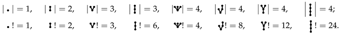
Trees are graphs such as , , , , , , , . The “root” of a tree is the lowest point in the diagram, and all vertices, except for the root, have a single parent. For a given tree t, the “order of t”, written as $|t|$, is the number of vertices in t. If a vertex v is the parent of $v^{\prime }$, then $v^{\prime }$ is a child of v. If there exists a path

$$(v_0,v_1,v_2,\dots ,v_n),\mathrm{where}{v}_i\mathrm{is}\mathrm{a}\mathrm{child}\mathrm{of}{v}_{i-1},i=1,2,\dots ,n,$$

then $v_n$ is a “descendant” of $v_0$. The product of the number of descendants for every vertex in a tree t is defined to be the “factorial of t” and is written as $t!$.

For the first eight trees, the order and factorial are the following:

2.1. Notation and Recursions

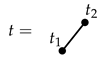
In this paper, $\tau$ := , and we recall two recursions to build other trees in terms of $\tau$. There are two convenient constructions for building complicated trees in terms of simpler trees. They are the following:

• Given trees $t_1$, $t_2$, …, $t_m$, define $t=[t_1{t}_2\cdots t_m]$ from the diagram

  

  The notation $\left[t_1^{k_1}{t}_2^{k_2}\dots t_m^{k_m}\right]$ is used to show repetitions of $t_1$, … Assuming the $t_i$ are distinct, then the “symmetry” $\sigma (t)$ is defined recursively by

  $$\begin{array}{cc}\hfill \sigma (\tau )& =1,\hfill \\ \hfill \sigma \left(\left[t_1^{k_1}{t}_2^{k_2}\cdots t_m^{k_m}\right]\right)& =\prod _{i=1}^m{k}_i!\sigma {(t_i)}^{k_i}.\hfill \end{array}$$
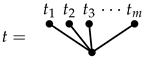
• Given trees $t_1$ and $t_2$, define $t=t_1\ast t_2$ from the diagram

  

2.2. Polish Notation Tree Construction

Polish notation or prefix (as distinct from infix or postfix) notation is credited to Lukasiewicz. A famous reference to his work is [5]. We generalise the notation so that ${\tau }_m$ acts as a prefix operator on m operands and thus ${\tau }_m{t}_1{t}_2\cdots t_m$ has the same meaning as $[t_1{t}_2\cdots t_m]$. This gives a third and bracketless scheme for writing trees. In Table 1, the various notations are given side by side. It is noted that the notation based on $t\ast t^{\prime }$ does not always give a unique factorisation.

Table 1. Tree notations.

Tree	Notation 1	Notation 2	Polish Notation
	$\tau$	$\tau$	$\tau$
	$[\tau ]$	$\tau \ast \tau$	${\tau }_1\tau$
	$[{\tau }^2]$	$(\tau \ast \tau )\ast \tau$	${\tau }_2\tau \tau$
	$[[\tau ]]$	$\tau \ast (\tau \ast \tau )$	${\tau }_1{\tau }_1\tau$
	$[{\tau }^3]$	$((\tau \ast \tau )\ast \tau )\ast \tau$	${\tau }_3\tau \tau \tau$
	$[\tau [\tau ]]$	$(\tau \ast \tau )\ast (\tau \ast \tau )=(\tau \ast (\tau \ast \tau ))\ast \tau$	${\tau }_2\tau {\tau }_1\tau$
	$[[{\tau }^2]]$	$\tau \ast ((\tau \ast \tau )\ast \tau )$	${\tau }_1{\tau }_2\tau \tau$
	$[[[\tau ]]]$	$\tau \ast (\tau \ast (\tau \ast \tau ))$	${\tau }_1{\tau }_1{\tau }_1\tau$

2.3. Elementary Differentials

Given an autonomous initial value problem,

$$y^{\prime }(x)=f(y(x)),y(x_0)=y_0,y:\mathbb{R}\to {\mathbb{R}}^N,f:{\mathbb{R}}^N\to {\mathbb{R}}^N,$$

(1)

we write $\mathbf{f}=(y_0)$ and also write the sequence of Fréchet derivatives of f, evaluated at $y_0$, as ${\mathbf{f}}^{\prime }$, ${\mathbf{f}}^{″}$, ${\mathbf{f}}^{(3)}$, … It is noted that, in linear algebra terms, these are linear, bilinear, and multilinear operators. In this paper, we always use Polish notation so that ${\mathbf{f}}^{(m)}$ acting on the m vectors $v_1$, $v_2$, …, $v_m$ is written as ${\mathbf{f}}^{(m)}{v}_1{v}_2\cdots v_m$.

Definition 1.

The elementary differential $\mathbf{F}(t)$ associated with the tree t is defined by

$$\begin{array}{cc}\hfill \mathbf{F}(\tau )& =\mathbf{f}\hfill \\ \hfill \mathbf{F}([t_1{t}_2\cdots t_m])& ={\mathbf{f}}^{(m)}\mathbf{F}(t_1)\mathbf{F}(t_2)\cdots \mathbf{F}(t_m).\hfill \end{array}$$

It is noted that the recursion formula can also be written as

$$\mathbf{F}({\tau }_m{t}_1{t}_2\cdots t_m)={\mathbf{f}}^{(m)}\mathbf{F}(t_1)\mathbf{F}(t_2)\cdots \mathbf{F}(t_m).$$

This makes it possible, in the Polish form of tree notation, to perform a simple substitution. That is, every $\tau$ is replaced by f, and every τ_m is replaced by f^(m).

2.4. Application to B-Series

Given a function $a:T\to \mathbb{R}$, the corresponding B-series is a formal Taylor series:

$$y_0+\sum _{t\in T}\frac{a(t)h^{|t|}}{\sigma (t)}\mathbf{F}(t).$$

Two special cases are the following:

• $t\mapsto 1/t!$, which gives the Taylor series for the solution to Equation (1) at $x=x_0+h$. The series is

  $$y_0+\sum _{t\in T}\frac{h^{|t|}}{t!\sigma (t)}\mathbf{F}(t).$$

  (2)
• $t\mapsto \mathsf{\Phi }(t)$, where $\mathsf{\Phi }(t)$ is the corresponding elementary weight for a specific Runge–Kutta method. This gives the Taylor series for the approximation computed by this Runge–Kutta method:

  $$y_0+\sum _{t\in T}\frac{\mathsf{\Phi }(t)h^{(|t|)}}{\sigma (t)}\mathbf{F}(t).$$

  (3)

By comparing Equations (2) and (3), we recover the conditions for a Runge–Kutta method to have order p:

$$\mathsf{\Phi }(t)=\frac{1}{t!},|t|\le p.$$

(4)

3. Trees, Forests, and Stumps

A sequence of items built from $\tau$, ${\tau }_1$, ${\tau }_2$, …, can be contracted by the rules of Polish operations to form a sequence of trees, together with a final subsequence that might not be a tree but would become one if further operands are appended on the right. The sequence of trees on the left is usually referred to as a forest and can be converted into a single tree by a suitable operator to the left of this subsequence.

Incomplete “trees” are referred to as stumps. Examples are

$${\tau }_1,{\tau }_2,{\tau }_2{\tau }_1\tau ,{\tau }_1{\tau }_2\tau ,{\tau }_1{\tau }_1{\tau }_1.$$

The “valency” of a stump is the number of copies of $\tau$, appended to the right, that would be required to convert it into a tree. It is convenient to refer to a tree as a stump with zero valency.

The word “forestump” is introduced to refer to a sequence of items made up from factors $\tau$ and ${\tau }_m$, $m=1,2,\dots$ When a particular forestump is contracted to form as many trees as possible, then the final form will be the formal product of a forest of trees followed by a single stump (possibly the empty stump).

3.1. Bicolour Diagrams to Represent Stumps

We now introduce a generalisation of the way trees are represented diagrammatically to include stumps. We regard stumps as modified trees with some leaves removed but with the edges from these missing leaves to their parents retained.

In the examples given here, a white disc represents the absence of a vertex. The number of white discs is the valency, with the remark that trees are stumps with zero valency.

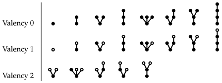
Right multiplication by one or more additional stumps implies grafting to open valency positions. It is noted that the third and fourth examples of valency 2 stumps are mirror images. This is significant in determining the precedence of the operands.

3.1.1. Products of Stumps

Given two stumps s and $s^{\prime }$, the product $s{s}^{\prime }$ has a nontrivial product if $s^{\prime }$ is not the trivial stump and s has valency of at least 1; that is, if s is not a tree, the product is formed by grafting the root of $s^{\prime }$ to the rightmost open valency in s.

Two examples of grafting illustrate the significance of stump orientations:

If s is a tree or $s^{\prime }$ is the trivial stump, no contraction takes place.

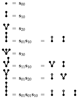
3.1.2. Atomic Stumps

An atomic stump is a graph of the following form:

It is noted that no more than two generations can be present.

If m of the children of the root are represented by black discs and n are represented by white discs, then the atomic stump is denoted by ${\mathrm{s}}_{mn}$. The reason for the designation “atomic” is that every tree can be written as the product of atoms.

This is illustrated for trees of up to order 4:

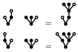
3.1.3. Isomeric Trees

In the factorisation of trees into products of atoms, the factors are written in a specific order, with each factor operating on later factors. However, if we interpret the atoms just as symbols that can commute with each other, we obtain a new equivalence relation, written as ∼.

Definition 2.

Two trees are isomeric if their atomic factors are the same.

Nothing interesting happens up to order 4, but for order 5, we find that

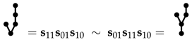
It is a simple exercise to find all isomeric classes of any particular order, but, as far as the author knows, this has not been done above order 6.

For orders 5 and 6, the isomers are, line by line, the following:

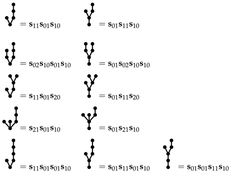
We see in Section 4 that isomeric classes for scalar differential equations have a similar role to individual trees in the case of differential systems of arbitrarily high dimension. We let $a_n$ denote the number of trees with order n and $A_n$ denote the accumulated total $a_1+a_2+\cdots +a_n$. Similarly, we let $b_n$ denote the number of isomeric classes with order n and $B_n$ denote the accumulated total for this quantity. These are shown in Table 2 up to order 6.

Table 2. Trees and isomeric classes for various orders.

n	1	2	3	4	5	6
$a_n$	1	1	2	4	9	20
$A_n$	1	2	4	8	17	37
$b_n$	1	1	2	4	8	15
$B_n$	1	2	4	8	16	31

4. Scalar Differential Equations

Early studies of Runge–Kutta methods derived order conditions for the scalar initial value problem

$$y^{\prime }(x)=f(x,y(x)),$$

(5)

instead of using the autonomous test problem (Equation (1)).

The full set of conditions up to some specified order becomes the starting point for finding accurate Runge–Kutta methods. The derivations of these conditions to order 5 were the pioneering contributions of Runge, Heun, and then Kutta [6,7,8]. We follow their arguments for the same model problem (Equation (5)). In this derivation, ${\partial }_{x}f:=\partial f/\partial x$ and ${\partial }_{y}f:=\partial f/\partial y$, with similar notations for higher partial derivatives. First, we find the second derivative of y by the chain rule:

$$y^{″}={\partial }_{x}f+({\partial }_{y}f)f.$$

Similarly, we find the third derivative:

$$\begin{array}{cc}\hfill y^{(3)}& =\left({\partial }_x^{2}f+({\partial }_x{\partial }_{y}f)f\right)+{\partial }_{y}f\left({\partial }_{x}f+({\partial }_{y}f)f\right)+({\partial }_x{\partial }_{y}f)f+({\partial }_y^{2}f)f^2\hfill \\ & ={\partial }_x^{2}f+2({\partial }_x{\partial }_{y}f)f+({\partial }_y^{2}f)f^2+({\partial }_{x}f{\partial }_{y}f)f+{({\partial }_{y}f)}^{2}f\hfill \end{array}$$

and carry on to find fourth and higher derivatives. By evaluating $y^{(n)}$ at $x=x_0$, we can find the Taylor expansions to use in Equation (5). A more complicated calculation leads to the detailed series of Equation (8) in the case of any particular Runge–Kutta method and hence to the determination of its order. We pursue this line of enquiry below.

The greatest achievement in this line of work was given in [3], where sixth order methods involving eight stages were derived. In all the derivations of new methods, up to the publication of this tour de force, a tacit assumption was made. This was that a method derived to have a specific order for a general scalar problem will have this same order for a coupled system of scalar problems; that is, it will have this order for a problem with $N>1$. This bald assumption is untrue, and it becomes necessary to carry out the order analysis in a multidimensional setting.

4.1. Nonautonomous Vector-Valued Problems

This analysis was carried out in a scalar context, in contrast to later work, for which the application was always to vector-valued problems. To cater for problems that are both nonautonomous and, at the same time, vector-valued, we can use the terminology of the present section but with a multidimensional interpretation.

This is done by regarding factors such as ${\partial }_{y}f$ and ${\partial }_y^{2}f$ as linear operators and bilinear operators, respectively, that operate on vector-valued terms to the right, using Polish notation. To maintain this interpretation, when a problem is nonscalar, this requires the strict order of factors to be observed. Of course, in the traditional scalar interpretation, all factors commute, and the order of factors could have been altered.

4.2. Systematic Derivation of Taylor Series

The evaluation of $y^{(n)}$, $n=1,2,\dots ,5$, is now carried out in a systematic manner. We let

$$D_{mn}=\sum _{i=0}^m\left(\genfrac{}{}{0pt}{}{m}{i}\right)({\partial }_x^{m-i}{\partial }_y^{n+i}f)f^i.$$

(6)

We also let ${\mathit{D}}_{mn}$ denote $D_{mn}$ evaluated at $(x_0,y_0)$.

Lemma 1.

$$\frac{\mathrm{d}}{\mathrm{d}x}{D}_{mn}=D_{m+1,n}+m{D}_{m-1,n+1}{D}_{10}.$$

(7)

Proof. 

$$\begin{array}{c}\frac{\mathrm{d}}{\mathrm{d}x}\sum _{i=0}^m\left(\genfrac{}{}{0pt}{}{m}{i}\right)({\partial }_x^{m-i}{\partial }_y^{n+i}f)f^i\hfill \\ =\left(\sum _{i=0}^m\left(\genfrac{}{}{0pt}{}{m}{i}\right)({\partial }_x^{m-i+1}{\partial }_y^{n+i}f)f^i+\sum _{i=0}^m\left(\genfrac{}{}{0pt}{}{m}{i}\right)({\partial }_x^{m-i}{\partial }_y^{n+i+1}f)f^{i+1}\right)+\sum _{i=0}^m\left(\genfrac{}{}{0pt}{}{m}{i}\right)i({\partial }_{x}f)({\partial }_x^{m-i}{\partial }_y^{n+i}{\partial }_{y}f)f^{i-1}\hfill \\ =\sum _{i=0}^{m+1}\left(\left(\genfrac{}{}{0pt}{}{m}{i}\right)+\left(\genfrac{}{}{0pt}{}{m}{i-1}\right)\right){\partial }_x^{m-i+1}({\partial }_y^{n+i}f)f^i+\sum _{i=0}^m\left(i\frac{m!}{i!(m-i)!}\right)({\partial }_{x}f)({\partial }_x^{m-i}{\partial }_y^{n+i}{\partial }_{y}f)f^{i-1}\hfill \\ =\sum _{i=0}^{m+1}\left(\genfrac{}{}{0pt}{}{m+1}{i}\right)({\partial }_x^{m-i+1}{\partial }_y^{n+i}f)f^i+m\sum _{i=0}^{m-1}\left(\genfrac{}{}{0pt}{}{m-1}{i}\right)({\partial }_{x}f)({\partial }_x^{m-i-1}{\partial }_y^{n+1+i}{\partial }_{y}f)f^i\hfill \\ =D_{m+1,n}+m{D}_{m-1,n+1}{D}_{10}.\hfill \end{array}$$

 ☐

Using Lemma 1, we find in turn that

$$\begin{array}{cc}\hfill y^{\prime }& =D_{00}\hfill \\ \hfill y^{″}& =D_{10}\hfill \\ \hfill y^{‴}& =D_{20}+D_{01}{D}_{10}\hfill \\ \hfill y^{(4)}& =D_{30}+2D_{11}{D}_{10}+D_{11}{D}_{10}+D_{01}(D_{20}+D_{01}{D}_{10})\hfill \\ & =D_{30}+3D_{11}{D}_{10}+D_{01}{D}_{20}+D_{01}^2{D}_{10}\hfill \\ \hfill y^{(5)}& =D_{40}+3D_{21}{D}_{10}+3(D_{21}+D_{02}{D}_{10})D_{10}+3D_{11}(D_{20}+D_{01}{D}_{10})\hfill \\ & +D_{11}{D}_{20}+D_{01}(D_{30}+2D_{11}{D}_{10})+2D_{01}{D}_{11}{D}_{10}+D_{01}^2(D_{20}+D_{01}{D}_{10})\hfill \\ & =D_{40}+6D_{21}{D}_{10}+3D_{02}{D}_{10}{D}_{10}+4D_{11}{D}_{20}+7D_{11}{D}_{01}{D}_{10}\hfill \\ & +D_{01}{D}_{30}+D_{01}^2{D}_{20}+D_{01}^3{D}_{10}.\hfill \end{array}$$

(8)

To find the order conditions for a Runge–Kutta method, up to order 5, we need to systematically find the Taylor series for the stages and finally for the output. In this analysis, we assume that ${\sum }_{j=1}^s{a}_{ij}=c_i$ for all stages. For the stages, it is sufficient to work only to order 4, so that the scaled stage derivatives include $h^5$ terms.

As a step towards finding the Taylor expansions of the stages and the output, we need to find the series for $hf(Y)$ for a given series $Y=y_0+\cdots$. In the following result, we use an arbitrary weighted series using the terms in Equation (8).

Lemma 2.

If

$$\begin{array}{cc}\hfill Y& =y_0+a_{1}h{\mathit{D}}_{00}+a_2{h}^2{\mathit{D}}_{10}+a_3{h}^3\frac{1}{2}{\mathit{D}}_{20}+a_4{h}^3{\mathit{D}}_{01}{\mathit{D}}_{10}\hfill \\ & +a_5{h}^4\frac{1}{6}{\mathit{D}}_{30}+a_6{h}^4{\mathit{D}}_{11}{\mathit{D}}_{10}+a_7{h}^4\frac{1}{2}{\mathit{D}}_{01}{\mathit{D}}_{20}+a_8{h}^4{\mathit{D}}_{01}^2{\mathit{D}}_{10}+\mathcal{O}(h^5),\hfill \end{array}$$

then

$$hf(x_0+h{a}_1,Y)=h{T}_1+h^2{T}_2+h^3{T}_3+h^4{T}_4+h^5{T}_5+\mathcal{O}(h^6),$$

where

$$\begin{array}{cc}\hfill T_1& ={\mathit{D}}_{00},\hfill \\ \hfill T_2& =a_1{\mathit{D}}_{10},\hfill \\ \hfill T_3& =\frac{1}{2}{a}_1^2{\mathit{D}}_{20}+a_2{\mathit{D}}_{01}{\mathit{D}}_{10}\hfill \\ \hfill T_4& =\frac{1}{6}{a}_1^3{\mathit{D}}_{30}+a_1{a}_2{\mathit{D}}_{11}{\mathit{D}}_{10}+\frac{1}{2}{a}_3{\mathit{D}}_{01}{\mathit{D}}_{20}+a_4{\mathit{D}}_{01}^2{\mathit{D}}_{10}\hfill \\ \hfill T_5& =\frac{1}{24}{a}_1^4{\mathit{D}}_{40}+\frac{1}{2}{a}_1^2{a}_2{\mathit{D}}_{21}{\mathit{D}}_{10}+a_1{a}_3{\mathit{D}}_{11}{\mathit{D}}_{20}+\left(a_1{a}_4+a_6\right){\mathit{D}}_{11}{\mathit{D}}_{01}{\mathit{D}}_{10}\hfill \\ & +\frac{1}{2}{a}_2^2{\mathit{D}}_{02}{\mathit{D}}_{10}^2+\frac{1}{6}{a}_5{\mathit{D}}_{30}{\mathrm{D}}_{01}+\frac{1}{2}{a}_7{\mathit{D}}_{01}^2{\mathit{D}}_{20}+a_8{\mathit{D}}_{01}^3{\mathit{D}}_{10}.\hfill \end{array}$$

Proof. 

Throughout this proof, an expression of the form ${\partial }_x^k{\partial }_y^{m}f$ is assumed to have been evaluated at $(x_0,y_0)$. Evaluate $T_1$, $T_2$, $T_3$, and $T_4$:

$$T_{1}h+T_2{h}^2+T_3{h}^3+T_4{h}^4+\mathcal{O}(h^5),$$

where

$$\begin{array}{cc}\hfill T_1& =f(x_0,y_0)={\mathit{D}}_{00},\hfill \\ \hfill T_2& =a_1{\partial }_{x}f+a_1({\partial }_{y}f)f=a_1{\mathit{D}}_{10},\hfill \\ \hfill T_3& =\frac{1}{2}{a}_1^2{\partial }_x^{2}f+a_1^2({\partial }_x{\partial }_y){\mathit{D}}_{00}+\frac{1}{2}{a}_1^2({\partial }_y^{2}f){\mathit{D}}_{00}^2+a_2({\partial }_{y}f){\mathit{D}}_{10}\hfill \\ & =\frac{1}{2}{a}_1^2{\mathit{D}}_{20}+a_2{\mathit{D}}_{01}{\mathit{D}}_{10},\hfill \\ \hfill T_4& =\frac{1}{6}{a}_1^3{\partial }_x^{3}f+\frac{1}{2}{a}_1^3({\partial }_x^2{\partial }_{y}f){\mathit{D}}_{10}+\frac{1}{2}{a}_1^3({\partial }_x{\partial }_y^{2}f){\mathit{D}}_{10}^2+\frac{1}{6}{a}_1^3{\partial }_y^{3}f{\mathit{D}}_{10}^3\hfill \\ & +a_1{a}_2({\partial }_x{\partial }_{y}f){\mathit{D}}_{10}+a_1{a}_2({\partial }_y^{2}f){\mathit{D}}_{10}{\mathit{D}}_{01}+a_3({\partial }_{y}f){\mathit{D}}_{20}+a_4({\partial }_{y}f){\mathit{D}}_{01}{\mathit{D}}_{10}\hfill \\ & =\frac{1}{6}{a}_1^3{\mathit{D}}_{30}+a_1{a}_2{\mathit{D}}_{11}{\mathit{D}}_{10}+a_3{\mathit{D}}_{01}{\mathit{D}}_{20}+a_4{\mathit{D}}_{01}^2{\mathit{D}}_{10}.\hfill \end{array}$$

The evaluation of $T_5$ is similar but more complicated and is omitted. ☐

For the stage values of a Runge–Kutta method, we have

$$\begin{array}{cc}\hfill Y_i& =y_0+\sum _{j=1}^s{a}_{ij}hf(x_0+h{c}_j,Y_j)\hfill \\ & =y_0+h{c}_i{\mathit{D}}_{00}+\mathcal{O}(h^2)\hfill \end{array}$$

and then, to one further order,

$$\begin{array}{cc}\hfill Y_i& =y_0+\sum _{j=1}^s{a}_{ij}hf(x_0+h{c}_j,y_0+h{c}_j{\mathit{D}}_{00})+\mathcal{O}(h^3)\hfill \\ & =y_0+h{c}_i{\mathit{D}}_{00}+h^2\sum _j{a}_{ij}{c}_j{\mathit{D}}_{10}+\mathcal{O}(h^3).\hfill \end{array}$$

A similar expression can be written down for the output from a step:

$$y_1=y_0+h\sum _i{b}_i{\mathit{D}}_{00}+h^2\sum _i{b}_i{c}_i{\mathit{D}}_{10}+\mathcal{O}(h^3).$$

A comparison with the exact solution, $y_0+h{y}^{\prime }(x_0)+\frac{1}{2}{h}^2{y}^{″}(x_0)+\mathcal{O}(h^3)$, evaluated using Equation (8), gives, under second order conditions,

$$\begin{array}{cc}\hfill \sum _i{b}_i{\mathit{D}}_{00}& ={\mathit{D}}_{00},\hfill \\ \hfill \sum _i{b}_i{c}_i{\mathit{D}}_{10}& =\frac{1}{2}{\mathit{D}}_{10}.\hfill \end{array}$$

This analysis can be taken further in a straightforward and systematic way and is summarised, as far as order 5, in Theorem 1. This theorem, for which the detailed proof is omitted, has to be read together with Table 3.

Table 3. Data for Theorem 1 with reference numbers (O1)–(O11) and (O14)–(O17) shown.

p	$\mathit{\sigma }$	T	$\mathit{\varphi }=\mathit{e}$
1	1	${\mathit{D}}_{00}$	$\sum b_i=1$	(O1)
2	1	${\mathit{D}}_{10}$	$\sum b_i{c}_i=\frac{1}{2}$	(O2)
3	2	${\mathit{D}}_{20}$	$\sum b_i{c}_i^2=\frac{1}{3}$	(O3)
	1	${\mathit{D}}_{01}{\mathit{D}}_{10}$	$\sum b_i{a}_{ij}{c}_j=\frac{1}{6}$	(O4)
4	6	${\mathit{D}}_{30}$	$\sum b_i{c}_i^3=\frac{1}{4}$	(O5)
	1	${\mathit{D}}_{11}{\mathit{D}}_{10}$	$\sum b_i{c}_i{a}_{ij}{c}_j=\frac{1}{8}$	(O6)
	2	${\mathit{D}}_{01}{\mathit{D}}_{20}$	$\sum b_i{a}_{ij}{c}_j^2=\frac{1}{12}$	(O7)
	1	${\mathit{D}}_{01}^2{\mathit{D}}_{10}$	$\sum b_i{a}_{ij}{a}_{jk}{c}_k=\frac{1}{24}$	(O8)
5	24	${\mathit{D}}_{40}$	$\sum b_i{c}_i^4=\frac{1}{6}$	(O9)
	2	${\mathit{D}}_{21}{\mathit{D}}_{10}$	$\sum b_i{c}_i^2{a}_{ij}{c}_j=\frac{1}{10}$	(O10)
	2	${\mathit{D}}_{11}{\mathit{D}}_{20}$	$\sum b_i{c}_i{a}_{ij}{c}_j^2=\frac{1}{15}$	(O11)
	1	${\mathit{D}}_{11}{\mathit{D}}_{01}{\mathit{D}}_{10}$	$\sum b_i(c_i+c_j)a_{ij}{a}_{jk}{c}_k=\frac{7}{120}$
	2	${\mathit{D}}_{02}{\mathit{D}}_{10}^2$	$\sum b_i{a}_{ij}{c}_j{a}_{ik}{c}_k=\frac{1}{20}$	(O14)
	6	${\mathit{D}}_{01}{\mathit{D}}_{30}$	$\sum b_i{a}_{ij}{c}_3^3=\frac{1}{20}$	(O15)
	2	${\mathit{D}}_{01}^2{\mathit{D}}_{20}$	$\sum b_i{a}_{ij}{a}_{jk}{c}_k^2=\frac{1}{60}$	(O16)
	1	${\mathit{D}}_{01}^3{\mathit{D}}_{10}$	$\sum b_i{a}_{ij}{a}_{jk}{a}_{k\ell }{c}_{\ell }=\frac{1}{120}$	(O17)

Theorem 1.

In the statement of this result, the quantities p, $\mathit{T}$, σ, and ϕ are given in Table 3.

1.

The Taylor expansion for the exact solution to the initial value problem

$$y^{\prime }(x)=f(x,y),y(x_0)=y_0$$

(9)

to within $\mathcal{O}(h^6)$ is $y_0$ plus the sum of terms of the form

$$\mathit{e}{h}^p{\sigma }^{-1}\mathit{T}.$$

2.

The Taylor expansion for the numerical solution $y_1$ to Equation (9), using a Runge–Kutta method $(A,b^{\mathrm{T}},c)$, to within $\mathcal{O}(h^6)$ is $y_0$ plus the sum of terms of the form

$$\varphi h^p{\sigma }^{-1}\mathit{T}.$$

3.

The conditions to order 5, for the solution of Equation (5) using $(A,b^{\mathrm{T}},c)$, are the equations of the form

$$\varphi =\mathit{e}.$$

4.3. Order Conditions for Vector Problems

The order conditions for the autonomous vector problem, given by Equation (4) for $p=5$, are identical to (O1)–(O11) and (O14)–(O17) together with the two cases of (4) missing from Table 3:

$$\begin{array}{}\mathrm{(O12)}& \hfill \sum b_i{c}_i{a}_{ij}{a}_{jk}{c}_k& =\frac{1}{30},\hfill \mathrm{(O13)}& \hfill \sum b_i{a}_{ij}{c}_j{a}_{jk}{c}_k& =\frac{1}{40}.\hfill \end{array}$$

Although these do not occur in Table 3, the sum of (O12) and (O13) is equal to

$$\sum b_i(c_i+c_j)a_{ij}{a}_{jk}{c}_k=\frac{7}{120},$$

(10)

which does occur as an un-numbered entry in Table 3. Apart from this discrepancy, the order conditions for the scalar and vector problems exactly agree as far as order 5.

4.4. Derivation of Ambiguous Method

We now construct a method that has order 5 for a scalar problem but only order 4 for a vector-based problem. This means that all the conditions $\mathsf{\Phi }(t)=1/t!$ need to be satisfied for the 17 trees such that $|t|\le 5$, except for (O12) and (O13), which can be replaced by Equation (10). In constructing this method, it is convenient to introduce a vector $d^{\mathrm{T}}$ defined as

$$d^{\mathrm{T}}=b^{\mathrm{T}}A+b^{\mathrm{T}}C-b^{\mathrm{T}}.$$

This satisfies the property

$$d^{\mathrm{T}}{c}^{n-1}=0,n=1,2,3,4,$$

(11)

because

$$d^{\mathrm{T}}{c}^{n-1}=b^{\mathrm{T}}A{c}^{n-1}+b^{\mathrm{T}}{c}^n-b^{\mathrm{T}}{c}^{n-1}=\frac{1}{n(n+1)}+\frac{1}{n+1}-\frac{1}{n}=0.$$

In the method to be constructed, some assumptions are made. These are

$$\begin{array}{cc}\hfill \sum _{j=1}^{i-1}{a}_{ij}{c}_j& =\frac{1}{2}{c}_i^2,i\ne 2,3,\hfill \end{array}$$

(12)

$$\begin{array}{cc}\hfill c_6& =1,\hfill \end{array}$$

(13)

$$\begin{array}{cc}\hfill b_2=b_3& =0.\hfill \end{array}$$

(14)

From Equations (13) and (14) and some of the order conditions, it follows that ${\sum }_{i=1}^6{b}_i{c}_i(c_i-c_4)(c_i-c_5)(1-c_i)=0$, implying that $\frac{1}{120}(20c_4{c}_5-10(c_4+c_5)+4)=0$ and hence that $(\frac{1}{2}-c_4)(c_5-\frac{1}{2})=\frac{1}{20}$. We choose the convenient values $c_4=\frac{1}{4}$ and $c_5=\frac{7}{10}$ together with $c_2=\frac{1}{2}$ and $c_3=1$. The value of b is found from (O1), (O2), (O3), (O5), and (O9), and d is found from Equation (11) with the requirement that $d_6=0$. The results are

$$\begin{array}{cc}\hfill b& =\phantom{t}[\begin{array}{cccccc}\frac{1}{14}& 0& 0& \frac{32}{81}& \frac{250}{567}& \frac{5}{54}\end{array}],\hfill \\ \hfill d& =\theta [\begin{array}{cccccc}1& 7& \frac{7}{9}& -\frac{112}{27}& \frac{125}{27}& 0\end{array}],\hfill \end{array}$$

where $\theta$ is a parameter, assumed to be nonzero. The third row of A can be found from

$$d_2\left(-\frac{1}{2}{c}_2^2\right)+d_3\left(a_{32}{c}_2-\frac{1}{2}{c}_3^2\right)=0,$$

(15)

because, from several order conditions,

$$\begin{array}{cccccccc}\hfill d^{\mathrm{T}}\left(Ac-\frac{1}{2}{c}^2\right)& =b^{\mathrm{T}}{A}^{2}c\hfill & +b^{\mathrm{T}}CAc\hfill & -b^{\mathrm{T}}Ac\hfill & -\frac{1}{2}{b}^{\mathrm{T}}A{c}^2\hfill & -\frac{1}{2}{b}^{\mathrm{T}}{c}^3\hfill & +\frac{1}{2}{b}^{\mathrm{T}}{c}^2& \\ & =\frac{1}{24}\hfill & +\frac{1}{8}\hfill & -\frac{1}{6}\hfill & -\frac{1}{24}\hfill & -\frac{1}{8}\hfill & +\frac{1}{6}& =0.\end{array}$$

From Equation (15), it is found that $a_{32}=\frac{13}{4}$. The values of $a_{42}$ and $a_{52}$ can be written in terms of the other elements of rows 4 and 5 of A, and row 6 can be found in terms of the other rows. There are now four free parameters remaining ($a_{43}$, $a_{53}$, $a_{54}$, and $\theta$) and four conditions that are not automatically satisfied. These are (O11), (O16), (O17), and Equation (10). The solutions are given in the complete tableau.

$$\begin{array}{c}0\\ \frac{1}{2}& \frac{1}{2}\\ 1& -\frac{9}{4}\phantom{-}& \frac{13}{4}\\ \frac{1}{4}& \frac{9}{64}& \frac{5}{32}& -\frac{3}{64}\phantom{-}\\ \frac{7}{10}& \frac{63}{625}& \frac{259}{2500}& \frac{231}{2500}& \frac{252}{625}\\ 1& -\frac{27}{50}\phantom{-}& -\frac{139}{50}\phantom{-}& -\frac{21}{50}\phantom{-}& \frac{56}{25}& \frac{5}{2}\\ & \frac{1}{14}& 0& 0& \frac{32}{81}& \frac{250}{567}& \frac{5}{54}\end{array}$$

(16)

5. Numerical Test

A suitable single differential equation to test the order of convergence of this method, together with a closely related autonomous system, is

$$\begin{array}{cc}\hfill \frac{dy}{dx}& =\frac{y-x}{y+x},\hfill \end{array}$$

(17)

$$\begin{array}{cc}\hfill \frac{d}{dt}\left[\begin{array}{c}x\\ y\end{array}\right]& =\frac{1}{\sqrt{x^2+y^2}}\left[\begin{array}{c}y+x\\ y-x\end{array}\right]\hfill \end{array}$$

(18)

The solution of Equation (17), in parametric coordinates, is

$$\begin{array}{cc}\hfill x& =\xi (t):=tsin(ln(t)),\hfill \\ \hfill y& =\eta (t):=tcos(ln(t)),\hfill \end{array}$$

and this is also the solution to Equation (18).

Two experiments were carried out:

• The scalar problem (Equation (17)) was solved using the method of Equation (16) on the interval $[\xi (\pi /6),\xi (5{\pi }^{\prime }12)]$.
• The two-dimensional problem of Equation (18), using the same method, was solved on the interval $[\pi /6,5{\pi }^{\prime }12]$.

In each case, $n=10\times 2^i$ for $i=0,1,2,3,4$. The errors for the two methods and the various numbers of steps are shown in Table 4. Also shown are the errors for n steps divided by the error for $2n$ steps.

Table 4. Variation of global errors for a range of step sizes.

n	Problem 1 Error	Ratio	Problem 2 Error	Ratio
10	$5.3177\times {10}^{-7}$	30.956	$1.1830\times {10}^{-5}$	15.068
$10\times 2$	$1.7179\times {10}^{-8}$	31.402	$7.8506\times {10}^{-7}$	15.157
$10\times 2^2$	$5.4705\times {10}^{-10}$	31.679	$5.1794\times {10}^{-8}$	15.485
$10\times 2^3$	$1.7268\times {10}^{-11}$	31.788	$3.3448\times {10}^{-9}$	15.720
$10\times 2^4$	$5.4323\times {10}^{-13}$	—	$2.1278\times {10}^{-10}$	—

As expected, the numerical behaviour for experiment 1 was consistent with order 5. In contrast, for experiment 2, the numerical behaviour was consistent only with order 4.

6. Discussion

There is little scientific interest in the solution of scalar initial value problems, and there is no advantage in constructing numerical methods that are suitable only for this special class of problems. Hence, in the search for useful numerical methods, it is an advantage to use tree-based theory. The results presented here emphasise the danger of using scalar theory to derive methods of order higher than 4 because they could be incorrect.

References

- Butcher, J.C. B-Series; Algebraic Analysis of Numerical Methods; Springer: Berlin, Germany, In preparation.
- Butcher, J.C. Numerical Methods for Ordinary Differential Equations, 3rd ed.; John Wiley & Sons: Chichester, UK, 2016. [Google Scholar]
- Hut’a, A. Une amélioration de la méthode de Runge–Kutta–Nyström pour la résolution numérique des équations différentielles du premier ordre. Acta Fac. Nat. Univ. Comenian. Math. 1956, 1, 201–224. [Google Scholar]
- Butcher, J.C. On the integration processes of A.Hut’a. J. Austral. Math. Soc. 1963, 3, 202–206. [Google Scholar] [CrossRef]
- ukasiewicz, J.; Tarski, J. Investigations into the Sentential Calculus. Comp. Rend. Soc. Sci. Lett. Vars. 1930, 23, 31–32. (In German) [Google Scholar]
- Heun, K. Neue Methode zur approximativen Integration der Differentialgleichungen einer unabhängigen Veränderlichen. Z. Math. Phys. 1900, 45, 23–38. [Google Scholar]
- Kutta, W. Beitrag zur näherungsweisen Integration totaler Differentialgleichungen. Z. Math. Phys. 1901, 46, 435–453. [Google Scholar]
- Runge, C. Über die numerische Auflösung von Differentialgleichungen. Math. Ann. 1895, 46, 167–178. [Google Scholar] [CrossRef]
© 2018 by the author. Licensee MDPI, Basel, Switzerland. This article is an open access article distributed under the terms and conditions of the Creative Commons Attribution (CC BY) license (http://creativecommons.org/licenses/by/4.0/).