A Model for the Universe that Begins to Resemble a Quantum Computer

Abstract

This article presents a sequential growth model for the Universe that acts like a quantum computer. The basic constituents of the model are a special type of causal set (causet) called a c-causet. A c-causet is defined to be a causet that has a unique labeling. We characterize c-causets as those causets that form a multipartite graph or equivalently those causets whose elements are comparable whenever their heights are different. We show that a c-causet has precisely two c-causet offspring. It follows that there are $2^n$ c-causets of cardinality $n+1$. This enables us to classify c-causets of cardinality $n+1$ in terms of n-bits. We then quantize the model by introducing a quantum sequential growth process. This is accomplished by replacing the n-bits by n-qubits and defining transition amplitudes for the growth transitions. We mainly consider two types of processes, called stationary and completely stationary. We show that for stationary processes, the probability operators are tensor products of positive rank-one qubit operators. Moreover, the converse of this result holds. Simplifications occur for completely stationary processes. We close with examples of precluded events.

1. Introduction

One frequently hears people say that the Universe acts like a giant quantum computer, but when pressed, they are usually short on the details. This article attempts to begin giving these details. It should be emphasized that only a basic framework is presented, and much work remains to be done. If this idea is correct, then great benefits will result. One benefit is the better understanding of the Universe itself, and another is the ability to greatly increase our computational power.

We first present a theory of discrete quantum gravity in terms of causal sets (causets) [1,2,3]. Unlike previous sequential growth models, the basic elements of this theory are a special type of causet called a covariant causet (c-causet). A c-causet is defined to be a causet that has a unique labeling. That is, two different labelings of a c-causet are isomorphic. The restriction of a growth model to c-causets provides great simplifications. For example, every c-causet possesses a unique c-causet history and has precisely two covariant offspring. It follows that there are $2^n$ c-causets of cardinality $n+1$. This enables us to classify c-causets of cardinality $n+1$ in terms of n-bits. The framework of a classical computer is already emerging. We characterize c-causets as those causets that form a multipartite graph or equivalently those causets whose elements are comparable whenever their heights are different.

We next quantize the model by introducing a quantum sequential growth process. This is accomplished by replacing the n-bits with n-qubits and defining transition amplitudes for the growth transitions. The transition amplitudes are given by complex-valued coupling constants $c_{n,j}$, $j=0,1,\dots ,2^{n-1}$. If the coupling constants are independent of j, we call the process stationary, and if they are independent of n and j, we call the process completely stationary. We show that for stationary processes, the probability operators that determine the quantum dynamics are tensor products of rank-one qubit operators. Moreover, the converse of this result holds. Simplifications occur for completely stationary processes. In this case, all of the qubit operators are the same and can be related to spin operators. We close with some examples of precluded events in the completely stationary case.

2. Covariant Causets

In this article, we call a finite partially ordered set a causet. If two causets are order isomorphic, we consider them to be identical. If a and b are elements of a causet x, we interpret the order $a<b$ as meaning that b is in the causal future of a and a is in the causal past of b. An element $a\in x$ is maximal if there is no $b\in x$ with $a<b$. If $a<b$ and there is no $c\in x$ with $a<c<b$, then a is a parent of b and b is a child of a. If $a,b\in x$, we say that a and b are comparable if $a\le b$ or $b\le a$. A chain in x is a set of mutually comparable elements of x, and an antichain is a set of mutually incomparable elements of x. The height of $a\in x$ is the cardinality of the longest chain whose largest element is a. The height of x is the maximum of the heights of its elements. We denote the cardinality of x by $\left|x\right|$.

If x and y are causets with $\left|y\right|=\left|x\right|+1$, then x produces y if y is obtained from x by adjoining a single maximal element a to x. In this case, we write $y=x\uparrow a$ and use the notation $x\to y$. If $x\to y$, we also say that x is a producer of y and y is an offspring of x. In general, x may produce many offspring, and y may be the offspring of many producers.

A labeling for a causet x is a bijection $\ell :x\to \left\{1,2,\dots ,\left|x\right|\right\}$, such that $a,b\in x$ with $a<b$ implies that $\ell \left(a\right)<\ell \left(b\right)$. A labeled causet is a pair $(x,\ell )$, where ℓ is a labeling of x. For simplicity, we frequently write $x=(x,\ell )$ and call x an ℓ-causet. Two ℓ-causets x and y are isomorphic if there exists a bijection $\varphi :x\to y$, such that $a<b$ if and only if $\varphi \left(a\right)<\varphi \left(b\right)$ and $\ell \left[\varphi \left(a\right)\right]=\ell \left(a\right)$ for every $a\in x$. Isomorphic ℓ-causets are considered identical as ℓ-causets. It is not hard to show that any causet can be labeled in many different ways, but there are exceptions, and these are the ones of importance in this work. A causet is covariant if it has a unique labeling (up to ℓ-causet isomorphism). Covariance is a strong restriction, which says that the elements of the causet have a unique “birth order” up to isomorphism. We call a covariant causet a c-coset.

We denote the set of c-causets with cardinality n by ${\mathcal{P}}_n$ and the set of all c-causets by $\mathcal{P}=\cup {\mathcal{P}}_n$. Notice that any nonempty c-causet y has a unique producer. Indeed, if y had two different producers $x_1,x_2$, then $x_1$ and $x_2$ could be labeled differently, and these could be used to give different labelings for y. If $x\in \mathcal{P}$, then the parent-child relation $a\prec b$ makes x into a graph $(x,\prec )$. A graph G is multipartite if there is a partition of its vertices $V=\cup V_j$, such that the vertices of $V_j$ and $V_{j+1}$ are adjacent and there are no other adjacencies.

Theorem 2.1. The following statements for a causet x are equivalent. (a) x is covariant, (b) the graph $(x,\prec )$ is multipartite, (c) $a,b\in x$ are comparable whenever a and b have different heights.

Proof. Conditions (b) and (c) are clearly equivalent. To prove that (a) implies (b), suppose x is covariant and let $x={\cup }_{i=0}^m{y}_i$, where $y_i$ is the set of elements in x of height i. Suppose $a\in y_n$, $b\in y_{n+1}$ and $a\nless b$. We can delete maximal elements of y until b is maximal and the only element of height $n+1$. Denote the resulting causet by z. We can label b by $\left|z\right|$, a by $\left|z\right|-1$ and consistently label the other elements of z, so that z is an ℓ-causet. We can also label b by $\left|z\right|-1$, a by $\left|z\right|$ and keep the same labels for the other elements of z. This gives two nonisomorphic labelings of z. Adjoining maximal elements to z to obtain x, we have x with two nonisomorphic labelings, which is a contradiction. Hence, $a<b$ so a is a parent of b. It follows that x is multipartite. To prove that (b) implies (a), suppose the graph $(x,\prec )$ is multipartite. Letting $x={\cup }_{i=0}^m{y}_i$ where $y_i$ is the set of elements of height i, it follows that $a<b$ for all $a\in y_i$, $b\in y_{i+1}$, $i=0,\dots ,m-1$. We can write:

$$\begin{array}{cc}\hfill y_0& =\left\{a_1,\dots ,a_{\left|y_0\right|}\right\}\hfill \\ \hfill y_1& =\left\{a_{\left|y_0\right|+1},\dots ,a_{\left|y_0\right|+\left|y_1\right|}\right\}\hfill \\ \hfill ⋮& \\ \hfill y_m& =\left\{a_{\left|y_0\right|+\cdots +\left|y_{m-1}\right|+1},\dots ,a_{\left|y_0\right|+\cdots +\left|y_m\right|}\right\}\hfill \end{array}$$

where j is the label on $a_j$. This gives a labeling of x and is the only labeling up to isomorphism.  ☐

Theorem 2.2. If $x\in \mathcal{P}$, then x has precisely two covariant offspring.

Proof. By Theorem 2.1, the graph $(x,\prec )$ is multipartite. Suppose x has height n. Let $x_1=x\uparrow a$ where a has all of the elements of height n as parents. Then, a is the only element of $x_1$ with height $n+1$. Hence, $x_1$ is multipartite, so by Theorem 2.1, $x_1$ is a covariant offspring of x. Let $x_2=x\uparrow b$, where b has all of the elements of height $n-1$ in x as parents (if $n=1$, then b has no parents). It is clear that $x_2$ is a multipartite graph. By Theorem 2.1, $x_2$ is a covariant offspring of x. Furthermore, there is only one covariant offspring of each of these two types. Let $y=x\uparrow c$ be a covariant offspring of x that is not one of these two types, and let $a\in x$ have label $\left|x\right|$. Then, a and c are incomparable, and we can label c by $\left|x\right|+1$. If we interchange the labels of a and c, we get a nonisomorphic labeling of y, which gives a contradiction. We conclude that x has precisely two covariant offspring.   ☐

Corollary 2.3. There are $2^n$ c-causets of cardinality $n+1$.

Proof. Notice that we obtain all c-causets from the producer-offspring process of Theorem 2.2. Indeed, take any $x\in \mathcal{P}$ and delete maximal elements until we arrive at the one element c-causet. In this way, x is obtained from the process of Theorem 2.2. We now employ induction on n. There are $1=2^{1-1}$ c-causets of cardinality one. If the result holds for c-causets of cardinality n, then by Theorem 2.2, there are $2·2^{n-1}=2^n$ c-causets of cardinality $n+1$. Hence, the result holds for c-causets of cardinality $n+1$.   ☐

As a bonus, we obtain an already known combinatorial identity. A composition of a positive integer n is a sequence of positive integers whose sum is n. The order of terms in the sequence is taken into account. For example, the following are the compositions of $1,2,3,4,5$.

$$\begin{array}{cc}\hfill n& =1:1\hfill \\ \hfill n& =2:1+1,2\hfill \\ \hfill n& =3:1+1+1,1+2,2+1,3\hfill \\ \hfill n& =4:1+1+1+1,1+1+2,1+2+1,2+1+1,2+2,1+3,3+1,4\hfill \\ \hfill n& =5:1+1+1+1+1,1+1+1+2,1+1+2+1,1+2+1+1,\hfill \\ & 2+1+1+1,1+1+3,1+3+1,3+1+1,1+4,4+1,\hfill \\ & 2+3,3+2,1+2+2,2+1+2,2+2+1,5\hfill \end{array}$$

The reader has surely noticed that for $n=1,2,3,4,5$, the number of compositions of n is $2^{n-1}$.

Corollary 2.4. There are $2^{n-1}$ compositions of the positive integer n.

Proof. There is a bijection between compositions of n and multipartite graphs with n vertices. The result follows from Corollary 2.3.  ☐

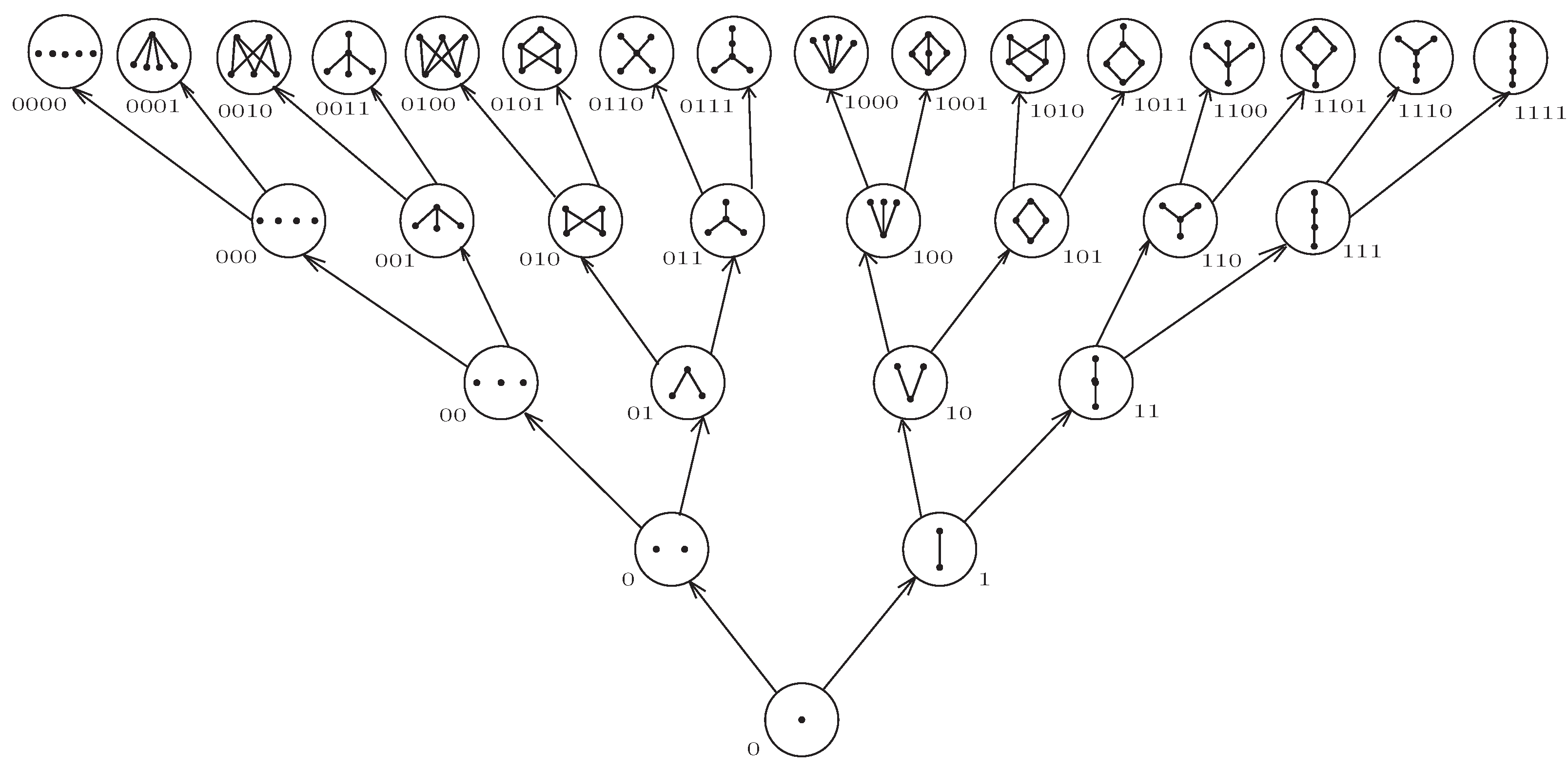
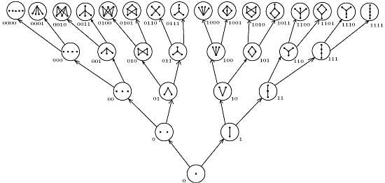
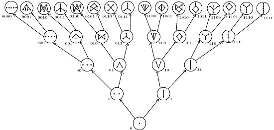
The pair $(\mathcal{P},\to )$ forms a partially ordered set in its own right. Moreover, $(\mathcal{P},\to )$ also forms a graph that is a tree. Figure 1 depicts the first five levels of this tree. The binary designations in Figure 1 will now be explained. By Corollary 2.3, at height $n+1$, there are $2^n$ c-causets, so binary numbers fit well, but how do we define a natural order for the c-causets? We have seen in Theorem 2.2 that if $x\in {\mathcal{P}}_n$, $n=1,2,\dots$, then x has precisely two offspring in $\mathcal{P}$, $x\to x_0,x_1$, where $x_0$ has the same height as x and $x_1$ has the height of x plus one. We call $x_0$ the 0-offspring and $x_1$ the 1-offspring of x. We assign a binary order to $x\in \mathcal{P}$ recursively as follows. If $x\in {\mathcal{P}}_1$, then x is the unique one element c-causet, and we designate x by 0. If $x\in {\mathcal{P}}_{n+1}$, then x has a unique producer $y\in {\mathcal{P}}_n$. Suppose y has binary order $j_{n-1}{j}_{n-2}\cdots j_2{j}_1$, $j_i=0$ or 1. If x is the 0-offspring of y, then we designate x with $j_{n-1}\cdots j_2{j}_{1}0$, and if x is a 1-offspring of y, then we designate x with $j_{n-1}\cdots j_2{j}_{1}1$. The reader can now check this definition with the binary order in Figure 1.

We now see the beginning development of a giant classical computer. At the $(n+1)$-th step of the process, n-bit strings are generated. It is estimated that we are now at about the ${10}^{60}$-th step, so $({10}^{60}-1)$-bit strings are being generated. There are about $2^{{10}^{60}}$ such strings, so an enormous amount of information is being processed. When we get to quantum computers, then superpositions of strings will be possible, and the amount of information increases exponentially. It is convenient to employ the notation:

$$\underline{j}=j_n{j}_{n-1}\cdots j_2{j}_1$$

for an n-bit string. In this way, we can designate each $x\in \mathcal{P}$ uniquely by $x_{n+1,\underline{j}}$, where $n+1=\left|x\right|$. For example, the c-causets at Step 3 in Figure 1 are $x_{3,00},x_{3,01},x_{3,10},x_{3,11}$. In decimal notation, we can also write these as $x_{3,0},x_{3,1}{x}_{3,2},x_{3,3}$.

Figure 1. Five Steps of a Multiverse

The binary order that we have just discussed is equivalent to a natural order in terms of the c-causet structure. Let $x=\left\{a_1,\dots ,a_n\right\}\in {\mathcal{P}}_n$, where we can assume without loss of generality that j is the label of $a_j$, $j=1,\dots ,n$. Define:

$$j_x\uparrow =\left\{i\in \mathbb{N}:a_j<a_i\right\}$$

Thus, $j_x\uparrow$ is the set of labels of the descendants of $a_j$. Order the set of c-cosets in ${\mathcal{P}}_n$ lexicographically as follows. If $x,y\in {\mathcal{P}}_n$, then $x<y$ if:

$$1_x\uparrow =1_y\uparrow ,\cdots ,j_x\uparrow =j_y\uparrow ,{(j+1)}_x\uparrow ⊊{(j+1)}_y\uparrow$$

It is easy to check that < is a total order relation on ${\mathcal{P}}_n$. The next theorem, whose proof we leave to the reader, shows that the order < on ${\mathcal{P}}_n$ is equivalent to the binary order previously discussed.

Theorem 2.5. If $x_{n,\underline{j}},x_{n,\underline{k}}\in {\mathcal{P}}_n$, then $x_{n\underline{j}}<x_{n,\underline{k}}$ if and only if $\underline{j}<\underline{k}$.

Example 1. We can illustrate Theorem 2.5 by considering ${\mathcal{P}}_4$. For the c-causets $x_{4,0},x_{4,1},\dots ,x_{4,7}\in {\mathcal{P}}_4$, we list the sets $(1_x\uparrow ,2_x\uparrow ,3_x\uparrow )$. Notice that we need not list $4_x\uparrow =\varnothing$ in all cases of ${\mathcal{P}}_4$.

$$\begin{array}{cc}\hfill x_{4,0}& :(\varnothing ,\varnothing ,\varnothing )\hfill \\ \hfill x_{4,1}& :(\left\{4\right\},\left\{4\right\},\left\{4\right\})\hfill \\ \hfill x_{4,2}& :(\left\{3,4\right\},\left\{3,4\right\},\varnothing )\hfill \\ \hfill x_{4,3}& :(\left\{2,3,4\right\},\left\{3,4\right\},\left\{4\right\})\hfill \\ \hfill x_{4,4}& :(\left\{2,3,4\right\},\varnothing ,\varnothing )\hfill \\ \hfill x_{4,5}& :(\left\{2,3,4\right\},\left\{4\right\},\left\{4\right\})\hfill \\ \hfill x_{4,6}& :(\left\{2,3,4\right\},\left\{3,4\right\},\varnothing )\hfill \\ \hfill x_{4,7}& :(\left\{2,3,4\right\},\left\{3,4\right\},\left\{4\right\})\hfill \end{array}$$

The lexicographical order becomes:

$$x_{4,0}<x_{4,1}<x_{4,2}<x_{4,3}<x_{4,4}<x_{4,5}<x_{4,6}<x_{x,7}$$

Example 2. This is so much fun, that we list the sets:

$$(1_x\uparrow ,2_x\uparrow ,3_x\uparrow ,4_x\uparrow )$$

for the c-causets $x_{5,0},\dots ,x_{5,15}\in {\mathcal{P}}_5$.

$$\begin{array}{cccc}\hfill x_{5,0}& :(\varnothing ,\varnothing ,\varnothing ,\varnothing )\hfill & \hfill x_{5,1}& :(\left\{5\right\},\left\{5\right\},\left\{5\right\},\left\{5\right\})\hfill \\ \hfill x_{5,2}& :(\left\{4,5\right\},\left\{4,5\right\},\left\{4,5\right\},\varnothing )\hfill & \hfill x_{5,3}& :(\left\{4,5\right\},\left\{4,5\right\},\left\{4,5\right\},\left\{5\right\})\hfill \\ \hfill x_{5,4}& :(\left\{3,4,5\right\},\left\{3,4,5\right\},\varnothing ,\varnothing )\hfill & \hfill x_{5,5}& :(\left\{3,4,5\right\},\left\{3,4,5\right\},\left\{5\right\},\left\{5\right\})\hfill \\ \hfill x_{5,6}& :(\left\{3,4,5\right\},\left\{3,4,5\right\},\left\{4,5\right\},\varnothing )\hfill & \hfill x_{5,7}& :(\left\{3,4,5\right\},\left\{3,4,5\right\},\left\{4,5\right\},\left\{5\right\})\hfill \\ \hfill x_{5,8}& :(\left\{2,3,4,5\right\},\varnothing ,\varnothing ,\varnothing )\hfill & \hfill x_{5,9}& :(\left\{2,3,4,5\right\},\left\{5\right\},\left\{5\right\},\left\{5\right\})\hfill \\ \hfill x_{5,10}& :(\left\{2,3,4,5\right\},\left\{4,5\right\},\left\{4,5\right\},\varnothing )\hfill & \hfill x_{5,11}& :(\left\{2,3,4,5\right\},\left\{4,5\right\},\left\{4,5\right\},\left\{5\right\})\hfill \\ \hfill x_{5,12}& :(\left\{2,3,4,5\right\},\left\{3,4,5\right\},\varnothing ,\varnothing )\hfill & \hfill x_{5,13}& :(\left\{2,3,4,5\right\},\left\{3,4,5\right\},\left\{5\right\},\left\{5\right\})\hfill \\ \hfill x_{5,14}& :(\left\{2,3,4,5\right\},\left\{3,4,5\right\},\left\{4,5\right\},\varnothing )\hfill & \hfill x_{5,15}& :(\left\{2,3,4,5\right\},\left\{3,4,5\right\},\left\{4,5\right\},\left\{5\right\})\hfill \end{array}$$

This order structure $({\mathcal{P}}_n,<)$ induces a topology on ${\mathcal{P}}_n$, whereby we can describe the “closeness” of c-causets. For example, we can place a metric on ${\mathcal{P}}_n$ by defining $\rho (x_{n\underline{j}},x_{n,\underline{k}})=\left|\underline{j}-\underline{k}\right|$. If we want to keep the size of the metric reasonable, we could define:

$$\rho (x_{n,\underline{j}},x_{n,\underline{k}})=\frac{1}{2^{n-1}}\left|\underline{j}-\underline{k}\right|$$

3. Quantum Sequential Growth Processes

The tree $(\mathcal{P},\to )$ can be thought of as a growth model, and an $x\in {\mathcal{P}}_n$ is a possible universe at step (time) n. An instantaneous universe x grows one element at a time in one of two ways at each step. A path in $\mathcal{P}$ is a sequence (string) ${\omega }_1{\omega }_2\cdots$ where ${\omega }_i\in {\mathcal{P}}_i$ and ${\omega }_i\to {\omega }_{i+1}$. An n-path is a finite sequence ${\omega }_1{\omega }_2\cdots {\omega }_n$, where, again, ${\omega }_i\in {\mathcal{P}}_i$ and ${\omega }_i\to {\omega }_{i+1}$. We denote the set of paths by Ω and the set of n-paths by ${\Omega }_n$. We think of $\omega \in \Omega$ as a “completed” universe or as a universal history. We may also view $\omega \in \Omega$ as an evolving universe. Since a c-causet has a unique producer, an n-path $\omega ={\omega }_1{\omega }_2\cdots {\omega }_n$ is completely determined by ${\omega }_n$. In other words, a c-causet possesses a unique history. We can thus identify ${\Omega }_n$ with ${\mathcal{P}}_n$, and we write ${\Omega }_n\approx {\mathcal{P}}_n$. If $\omega ={\omega }_1{\omega }_2\cdots {\omega }_n\in {\Omega }_n$, we denote by $(\omega \to )$ the two element subset of ${\Omega }_{n+1}$ consisting of $\left\{\omega x_0,\omega x_1\right\}$, where $x_0$ and $x_1$ are the offspring of ${\omega }_n$. Thus,

$$(\omega \to )=\left\{{\omega }_1\cdots {\omega }_n{x}_0,{\omega }_1\cdots {\omega }_n{x}_1\right\}$$

If $A\subseteq {\Omega }_n$, we define $(A\to )\subseteq {\Omega }_{n+1}$ by:

$$(A\to )=\cup \left\{(\omega \to ):\omega \in A\right\}$$

Thus, $(A\to )$ is the set of one-element continuations of n-paths in A.

The set of all paths beginning with $\omega \in {\Omega }_n$ is called an elementary cylinder set and is denoted by $\mathrm{cyl}\left(\omega \right)$. If $A\subseteq {\Omega }_n$, then the cylinder set $\mathrm{cyl}\left(A\right)$ is defined by:

$$\mathrm{cyl}\left(A\right)=\cup \left\{\mathrm{cyl}\left(\omega \right):\omega \in A\right\}$$

Using the notation:

$$\mathcal{C}\left({\Omega }_n\right)=\left\{\mathrm{cyl}\left(A\right):A\subseteq {\Omega }_n\right\}$$

we see that:

$$\mathcal{C}\left({\Omega }_1\right)\subseteq \mathcal{C}\left({\Omega }_2\right)\subseteq \cdots$$

is an increasing sequence of subalgebras of the cylinder algebra $\mathcal{C}(\Omega )=\cup \mathcal{C}\left({\Omega }_n\right)$. Letting $\mathcal{A}$ be the σ-algebra generated by $\mathcal{C}(\Omega )$, we have that $(\Omega ,\mathcal{A})$ is a measurable space. For $A\subseteq \Omega$, we define the sets $A^n\subseteq {\Omega }_n$ by:

$$A^n=\left\{{\omega }_1{\omega }_2\cdots {\omega }_n:{\omega }_1{\omega }_2\cdots {\omega }_n{\omega }_{n+1}\cdots \in A\right\}$$

That is, $A^n$ is the set of n-paths that can be continued to a path in A. We think of $A^n$ as the n-step approximation to A. We have that:

$$\mathrm{cyl}\left(A_1\right)\supseteq \mathrm{cyl}\left(A_2\right)\supseteq \cdots \supseteq A$$

so that $A\subseteq \cap \mathrm{cyl}\left(A^n\right)$. However, $A\ne \cap \mathrm{cyl}\left(A^n\right)$ in general, even if $A\in \mathcal{A}$.

Let $H_n=L_2\left({\Omega }_n\right)=L_2\left({\mathcal{P}}_n\right)$ be the n-path Hilbert space ${\mathbb{C}}^{{\Omega }_n}={\mathbb{C}}^{{\mathcal{P}}_n}$ with the usual inner product:

$$⟨f,g⟩=\sum \left\{\overline{f\left(\omega \right)}g\left(\omega \right):\omega \in {\Omega }_n\right\}$$

For $A\subseteq {\Omega }_n$, the characteristic function ${\chi }_A\in H_n$ has norm $\parallel {\chi }_A\parallel =\sqrt{\left|A\right|}$. In particular, $1_n={\chi }_{{\Omega }_n}$ satisfies:

$$\parallel 1_n\parallel ={\left|{\Omega }_n\right|}^{1/2}=2^{(n-1)/2}$$

A positive operator ρ on $H_n$ that satisfies $⟨\rho 1_n,1_n⟩=1$ is called a probability operator [1]. Corresponding to a probability operator ρ, we define the decoherence functional [1,4,5]:

$$D_{\rho }:2^{{\Omega }_n}\times 2^{{\Omega }_n}\to \mathbb{C}$$

by $D_{\rho }(A,B)=⟨\rho {\chi }_B,{\chi }_A⟩$. We interpret $D_{\rho }(A,B)$ as a measure of the interference between the events A and B when the system is described by ρ. We also define the q-measure ${\mu }_{\rho }:2^{{\Omega }_n}\to {\mathbb{R}}^{+}$ by ${\mu }_{\rho }\left(A\right)=D_{\rho }(A,A)$ and interpret ${\mu }_{\rho }\left(A\right)$ as the quantum propensity of the event $A\subseteq {\Omega }_n$ [1,3,6]. In general, ${\mu }_{\rho }$ is not additive on $2^{{\Omega }_n}$, so ${\mu }_{\rho }$ is not a measure. However, ${\mu }_{\rho }$ is Grade-2 additive [1,3,6] in the sense that if $A,B,C\in 2^{{\Omega }_n}$ are mutually disjoint, then:

$${\mu }_{\rho }(A\cup B\cup C)={\mu }_{\rho }(A\cup B)+{\mu }_{\rho }(A\cup C)+{\mu }_{\rho }(B\cup C)-{\mu }_{\rho }\left(A\right)-{\mu }_{\rho }\left(B\right)-{\mu }_{\rho }\left(C\right)$$

Let ${\rho }_n$ be a probability operator on $H_n$, $n=1,2,\dots$. We say that the sequence $\left\{{\rho }_n\right\}$ is consistent if:

$$D_{{\rho }_{n+1}}(A\to ,B\to )=D_{{\rho }_n}(A,B)$$

for all $A,B\subseteq {\Omega }_n$ [1]. We call a consistent sequence $\left\{{\rho }_n\right\}$ a covariant quantum sequential growth process (CQSGP). Let ${\rho }_n$ be a CQSGP and denote the corresponding q-measure by ${\mu }_n$. A set $A\in \mathcal{A}$ is suitable if $lim{\mu }_n\left(A^n\right)$ exists (and is finite), in which case, we define $\mu \left(A\right)=lim{\mu }_n\left(A^n\right)$. We denote the collection of suitable sets by $\mathcal{S}(\Omega )$. Of course, $\varnothing ,\Omega \in \mathcal{S}(\Omega )$ with $\mu \left(\varnothing \right)=0$, $\mu (\Omega )=1$. If $A\in \mathcal{C}(\Omega )$ and $A=\mathrm{cyl}\left(B\right)$, where $B\subseteq {\Omega }_m$, then it follows from consistency that $lim{\mu }_n\left(A^n\right)={\mu }_m\left(B\right)$. Hence, $A\in \mathcal{S}(\Omega )$ and $\mu \left(A\right)={\mu }_m\left(B\right)$. We conclude that $\mathcal{C}(\Omega )\subseteq \mathcal{S}(\Omega )\subseteq \mathcal{A}$, and it can be shown that the inclusions are proper, in general. In a sense, μ is a q-measure on $\mathcal{S}(\Omega )$ that extends the q-measures ${\mu }_n$.

There are physically relevant sets that are not in $\mathcal{C}(\Omega )$. In this case, it is important to know whether such a set A is in $\mathcal{S}(\Omega )$ and, if it is, to find $\mu \left(A\right)$. For example, if $\omega \in \Omega$, then:

$$\left\{\omega \right\}=\bigcap _{n=1}^{\infty }{\left\{\omega \right\}}^n\in \mathcal{A}$$

but $\left\{\omega \right\}\notin \mathcal{C}(\Omega )$. As another example, the complement ${\left\{\omega \right\}}^{\prime }\notin \mathcal{C}(\Omega )$. Even if $\left\{\omega \right\}\in \mathcal{S}(\Omega )$, since ${\mu }_n\left(A^{\prime }\right)\ne 1-{\mu }_n\left(A\right)$ for $A\subseteq {\Omega }_n$ in general, it does not follow immediately that ${\left\{\omega \right\}}^{\prime }\in \mathcal{S}(\Omega )$. For this reason, we would have to treat ${\left\{\omega \right\}}^{\prime }$ as a separate case.

We saw in Section 2 that we can represent each element of $\mathcal{P}$ uniquely as $x_{n,\underline{j}}$, where $n=\left|x\right|$ and $\underline{j}$ can be considered as a binary number. We can also represent each element in ${\mathcal{P}}_{n+1}$ as a n-bit binary number $\underline{j}=j_n{j}_{n-1}\cdots j_2{j}_1$, $j=0$ or 1. Since ${\Omega }_n\approx {\mathcal{P}}_n$, we can also represent each $\omega \in {\Omega }_{n+1}$ by an n-bit binary number $\underline{j}$. The standard basis for $H_{n+1}=L_2\left({\Omega }_{n+1}\right)$ is the set of vectors $e_{\underline{j}}={\chi }_{{\omega }_{\underline{j}}}$, ${\omega }_{\underline{j}}\in {\Omega }_{n+1}$. We frequently use the notation $\left|\underline{j}\right.⟩=e_{\underline{j}}$, which is called the computational basis in quantum computation theory. In this theory, $\left|\underline{j}\right.⟩$ is represented by:

$$\left|\underline{j}\right.⟩=\left|j_n\cdots j_2{j}_1\right.⟩=\left|j_n\right.⟩\otimes \cdots \otimes \left|j_2\right.⟩\otimes \left|j_1\right.⟩$$

where $\left|j_i\right.⟩$ is $\left|0\right.⟩$ or $\left|1\right.⟩$, which form the basis of the two-dimensional Hilbert space ${\mathbb{C}}^2$.

The basis vectors $\left|0\right.⟩$ and $\left|1\right.⟩$ are called qubit states, but we shall call them qubits, for short. We also call $\left|\underline{j}\right.⟩$, given above, an n-qubit. This is the quantum computation analogue of an n-bit of classical computer science. If ${\rho }_{n+1}$ is a probability operator, the corresponding decoherence matrix is the $2^n\times 2^n$ complex matrix, whose $\underline{j}-\underline{k}$ component is given by:

$$M_{{\rho }_{n+1}}=\left[⟨{\rho }_n\left|\underline{k}\right.⟩,\left|\underline{j}\right.⟩⟩\right]$$

This is frequently shortened to:

$$M_{{\rho }_{n+1}}=\left[⟨{\rho }_n\underline{k},\underline{j}⟩\right]$$

but we shall not use this notation, because it can be confusing. For $A,B\subseteq {\Omega }_{n+1}$, we form the superpositions:

$$\begin{array}{cc}\hfill \left|A\right.⟩& =\sum \left\{\left|\underline{i}\right.⟩:{\omega }_{\underline{i}}\in A\right\}\hfill \\ \hfill \left|B\right.⟩& =\sum \left\{\left|\underline{i}\right.⟩:{\omega }_{\underline{i}}\in B\right\}\hfill \end{array}$$

The decoherence functional is now given by:

$$D_{{\rho }_{n+1}}(A,B)=⟨{\rho }_{n+1}\left|B\right.⟩,\left|A\right.⟩⟩$$

Superpositions are a strictly quantum phenomenon that has no counterpart in classical computation.

An event $A\subseteq {\Omega }_n$ is precluded if ${\mu }_n\left(A\right)=0$ [6]. Precluded events have been extensively studied in [2,3,4,7,8], and they are considered to be events that never occur. We shall give simple examples later that show that if A is precluded and $B\subseteq A$, then B need not be precluded. However, the following properties do hold.

Theorem 3.1. (a) If $A\subseteq {\Omega }_n$ is precluded and $B\subseteq {\Omega }_n$ is disjoint from A, then ${\mu }_n(A\cup B)={\mu }_n\left(B\right)$. (b) If $A,B\subseteq {\Omega }_n$ are disjoint precluded events, then $A\cup B$ is precluded.

Proof. (a) Since ${\mu }_n\left(A\right)=0$, we have that:

$$\parallel {\rho }_n^{1/2}{\chi }_A{\parallel }^2=⟨{\rho }_n^{1/2}{\chi }_A,{\rho }_n^{1/2}{\chi }_A⟩=⟨{\rho }_n{\chi }_A,{\chi }_A⟩=0$$

Hence, ${\rho }_n^{1/2}{\chi }_A=0$ so ${\rho }_n{\chi }_A=0$. Since, $A\cap B=\varnothing$, we have that:

$$\begin{array}{cc}\hfill {\mu }_n(A\cup B)& =⟨{\rho }_n{\chi }_{A\cup B},{\chi }_{A\cup B}⟩=⟨{\rho }_n({\chi }_A+{\chi }_B),{\chi }_A+{\chi }_B⟩\hfill \\ & =⟨{\rho }_n{\chi }_A,{\chi }_A⟩+2\mathrm{Re}⟨{\rho }_n{\chi }_A,{\chi }_B⟩+⟨{\rho }_n{\chi }_B,{\chi }_B⟩\hfill \\ & =⟨{\rho }_n{\chi }_B,{\chi }_B⟩={\mu }_n\left(B\right)\hfill \end{array}$$

Part (b) follows from (a).  ☐

An event $A\in \mathcal{S}(\Omega )$ is precluded if $\mu \left(A\right)=0$ and A is strongly precluded if there exists an $n\in \mathbb{N}$, such that ${\mu }_m\left(A^m\right)=0$ for all $m\ge n$. For example, if $A=\mathrm{cyl}\left(B\right)$, where $B\subseteq {\Omega }_n$ and ${\mu }_n\left(B\right)=0$, then A is strongly precluded. Of course, strongly precluded events are precluded.

A precluded event is primitive if it has no proper, nonempty precluded subsets.

Theorem 3.2. If $A\subseteq {\Omega }_n$ is precluded, then A is primitive or A is a union of mutually disjoint primitive precluded events.

Proof. If A is primitive, we are finished. Otherwise, there exists a proper, nonempty precluded subset $B\subseteq A$. Since $\left|B\right|<\infty$, there exists a nonempty, primitive precluded event $A_1\subseteq B\subseteq A$. Applying Theorem 3.1, we conclude that ${\mu }_n(A\cap A_1^{\prime })=0$. In a similar way, there exists a nonempty, primitive precluded event $A_2\subseteq A\cap A_1^{\prime }$. Of course, $A_1\cap A_2=\varnothing$. Continuing, this process must eventually stop, and we obtain a sequence of mutually disjoint primitive preluded events $A_1,\dots ,A_n$ with $A=\cup A_i$.   ☐

4. Covariant Amplitude Processes

This section considers a method of constructing a CQSGP called a covariant amplitude process. Not all CQSGPs can be constructed in this way, but this method appears to have physical motivation [1].

A transition amplitude is a map $\tilde{a}:\mathcal{P}\times \mathcal{P}\to \mathbb{C}$, such that $\tilde{a}(x,y)=0$ if $x\nrightarrow y$ and ${\sum }_y\tilde{a}(x,y)=1$ for all $x\in \mathcal{P}$. This is similar to a Markov chain, except $\tilde{a}(x,y)$ may be complex. The covariant amplitude process (CAP) corresponding to $\tilde{a}$ is given by the maps $a_n:{\Omega }_n\to \mathbb{C}$ where:

$$a_n({\omega }_1{\omega }_2\cdots {\omega }_n)=\tilde{a}({\omega }_1,{\omega }_2)\tilde{a}({\omega }_2,{\omega }_3)\cdots \tilde{a}({\omega }_{n-1},{\omega }_n)$$

We can consider $a_n$ to be a vector in $H_n=L_2\left({\Omega }_n\right)=L_2\left({\mathcal{P}}_n\right)$. Notice that for $x\in {\mathcal{P}}_n$, we can define $a_n\left(x\right)$ to be $a_n\left(\omega \right)$, where $\omega \in {\Omega }_n$ is the unique history of x. Observe that:

$$⟨1_n,a_n⟩=\sum _{\omega \in {\Omega }_n}{a}_n\left(\omega \right)=1$$

and we also have that:

$$\parallel a_n\parallel ={\left(\sum _{\omega \in {\Omega }_n}{\left|a_n\left(\omega \right)\right|}^2\right)}^{1/2}$$

Define the rank-one positive operator ${\rho }_n=\left|a_n\right.⟩\left.⟨a_n\right|$ on $H_n$. The norm of ${\rho }_n$ is:

$$\parallel {\rho }_n\parallel =\parallel a_n{\parallel }^2=\sum _{\omega \in {\Omega }_n}{\left|a_n\left(\omega \right)\right|}^2$$

Since $⟨{\rho }_n{1}_n,1_n⟩={\left|⟨1_n,a_n⟩\right|}^2=1$, we conclude that ${\rho }_n$ is a probability operator. It is shown in [1] that $\left\{{\rho }_n\right\}$ is consistent, so $\left\{{\rho }_n\right\}$ forms a CQSGP. We call $\left\{{\rho }_n\right\}$ the CQSGP generated by the CAP $\left\{a_n\right\}$.

The decoherence functional corresponding to the CAP $\left\{a_n\right\}$ becomes:

$$\begin{array}{cc}\hfill D_n(A,B)& =⟨{\rho }_n{\chi }_B,{\chi }_A⟩=⟨{\chi }_B,a_n⟩⟨a_n,{\chi }_A⟩\hfill \\ & =\sum _{\omega \in A}\overline{a_n\left(\omega \right)}\sum _{\omega \in B}{a}_n\left(\omega \right)\hfill \end{array}$$

In particular, for $\omega ,{\omega }^{\prime }\in {\Omega }_n$, the decoherence matrix elements:

$$D_n(\omega ,{\omega }^{\prime })=\overline{a_n\left(\omega \right)}{a}_n\left({\omega }^{\prime }\right)$$

are the matrix elements of ${\rho }_n$ in the standard basis. The q-measure ${\mu }_n:2^{{\Omega }_n}\to {\mathbb{R}}^{+}$ is given by:

$${\mu }_n\left(A\right)=D_n(A,A)={\left|\sum _{\omega \in A}{a}_n\left(\omega \right)\right|}^2$$

In particular, ${\mu }_n\left(\omega \right)={\left|a_n\left(\omega \right)\right|}^2$ for every $\omega \in {\Omega }_n$ and ${\mu }_n\left({\Omega }_n\right)=1$. Of course, we also have that ${\mu }_n\left(x\right)={\left|a_n\left(x\right)\right|}^2$ for all $x\in {\mathcal{P}}_n$.

Since each $x\in {\mathcal{P}}_n$ has precisely two offspring, we can describe a transition amplitude $\tilde{a}$ and the corresponding CAP $\left\{a_n\right\}$ in a simple way. Let:

$$\begin{array}{cc}\hfill \tilde{a}(x_{n,\underline{j}},x_{n+1,\underline{j}0})& =c_{n,\underline{j}}\hfill \end{array}$$

and

$$\begin{array}{cc}\hfill \tilde{a}(x_{n,\underline{j}},x_{n+1,\underline{j}0})& =1-c_{n,\underline{j}}\hfill \end{array}$$

$j=0,1,\dots ,2^{n-1}-1$. We call the numbers $c_{n,\underline{j}}\in \mathbb{C}$ coupling constants for the corresponding CAP $\left\{a_n\right\}$.

Example 3. If the CAP $\left\{a_n\right\}$ has coupling constants $c_{n,\underline{j}}$, then we have $a_2\left(x_{2,0}\right)=c_{1,0}$, $a_2\left(x_{2,1}\right)=1-c_{1,0}$, $a_3\left(x_{3,00}\right)=c_{1,0}{c}_{2,0}$, $a_3\left(x_{3,01}\right)=c_{1,0}(1-c_{2,0})$, $a_3\left(x_{3,10}\right)=(1-c_{1,0})c_{2,1}$, $a_3\left(x_{3,11}\right)=(1-c_{1,0})(1-c_{2,1})$.

We shall only need a special case of the next theorem, but it still has independent interest.

Theorem 4.1. An operator M on $H_n$ is a rank-one probability operator if and only if M has a matrix representation $M=\left[{\overline{\alpha }}_j{\alpha }_k\right]$, where ${\alpha }_j\in \mathbb{C}$, $j=1,\dots ,n$, satisfy $\sum {\alpha }_j=1$.

Proof. Suppose $M=\left[M_{jk}\right]$ with $M_{jk}={\overline{\alpha }}_j{\alpha }_k$, where $\sum {\alpha }_j=1$. Let $\psi \in {\mathbb{C}}^n$ be the vector $\psi =({\alpha }_1,\dots ,{\alpha }_n)$. We have that $M=\left|\psi \right.⟩\left.⟨\psi \right|$, so M is positive with rank-one. To show that M is a probability operator, we have:

$$\sum _{j,k}{M}_{jk}=\sum _{j,k}{\overline{\alpha }}_j{\alpha }_k={\left|\sum {\alpha }_j\right|}^2=1$$

Conversely, let M be a rank-one probability operator. Since M is rank-one, it has the form $M=\left|\psi \right.⟩\left.⟨\psi \right|$ for some $\psi \in {\mathbb{C}}^n$. We then have the matrix representation:

$$M=\left[⟨e_j,\psi ⟩⟨\psi ,e_k⟩\right]$$

where $e_j$, $j=1,\dots ,n$, is the standard basis for ${\mathbb{C}}^n$. Letting ${\alpha }_j=⟨\psi ,e_j⟩$, we conclude that $M=\left[{\overline{\alpha }}_j{\alpha }_k\right]$. Since M is a probability operator, we have that:

$${\left|\sum _j{\alpha }_j\right|}^2=\sum _{j,k}{\overline{\alpha }}_j{\alpha }_k=1$$

Now, there exists a $\theta \in \mathbb{R}$, such that $e^{-i\theta }\sum {\alpha }_j=1$. Letting ${\psi }^{\prime }=e^{i\theta }\psi$, we obtain:

$$M=\left|{\psi }^{\prime }\right.⟩\left.⟨{\psi }^{\prime }\right|=\left[{\overline{\alpha }}_j^{\prime }{\alpha }_k^{\prime }\right]$$

where ${\alpha }_j^{\prime }=e^{-i\theta }{\alpha }_j$, $j=1,\dots ,n$. Hence, $\sum {\alpha }_j^{\prime }=1$.   ☐

An operator on ${\mathbb{C}}^2$ is called a qubit operator. We shall only need the following corollary of Theorem 4.1.

Corollary 4.2. A qubit operator M is a rank-one probability operator if and only if M has a matrix representation:

$$M=\left[\begin{array}{cc}{\left|c\right|}^2& \overline{c}(1-c)\\ c(1-\overline{c})& {\left|1-c\right|}^2\end{array}\right]$$

(4.1)

where $\alpha \in \mathbb{C}$.

A CAP $\left\{a_n\right\}$ is stationary if the coupling constants $c_{n,\underline{j}}$ are independent of j. In this case, we write $c_{n,\underline{j}}=c_n$, and we have $\tilde{a}(x_{n,\underline{j}},x_{n+1,\underline{j}0})=c_n,\tilde{a}(x_{n,\underline{j}},x_{n+1,\underline{j}1})=1-c_n$. By Corollary 4.2, the operators:

$${\widehat{c}}_j=\left[\begin{array}{cc}{\left|c_j\right|}^2& {\overline{c}}_j(1-c_j)\\ c_j(1-{\overline{c}}_j)& {\left|1-c_j\right|}^2\end{array}\right]$$

are qubit rank-one probability operators.

Theorem 4.3. Let $\left\{c_n\right\}$ be the coupling constants for a stationary CAP. The generated CQSGP $\left\{{\rho }_n\right\}$ has the form:

$${\rho }_n={\widehat{c}}_{n-1}\otimes {\widehat{c}}_{n-2}\otimes \cdots \otimes {\widehat{c}}_2\otimes {\widehat{c}}_1$$

(4.2)

Proof. Since ${\Omega }_n\approx {\mathcal{P}}_n$, we can write:

$${\rho }_2=D_2=\left[\begin{array}{cc}{\left|c_1\right|}^2& {\overline{c}}_1(1-c_1)\\ c_1(1-{\overline{c}}_1)& {\left|1-c_1\right|}^2\end{array}\right]={\widehat{c}}_1$$

At the next step, we apply Example 3 to obtain:

$$\begin{array}{cc}& {\rho }_3=D_3\hfill \\ & =\left[\begin{array}{cccc}{\left|c_1\right|}^2{\left|c_2\right|}^2& {\left|c_1\right|}^2{\overline{c}}_2(1-c_2)& {\overline{c}}_1(1-c_1){\left|c_2\right|}^2& {\overline{c}}_1(1-c_1){\overline{c}}_2(1-c_2)\\ {\left|c_1\right|}^2{c}_2(1-{\overline{c}}_2)& {\left|c_1\right|}^2{\left|1-c_2\right|}^2& {\overline{c}}_1(1-c_1)c_2(1-{\overline{c}}_2)& {\overline{c}}_1(1-c_1){\left|1-c_2\right|}^2\\ c_1(1-{\overline{c}}_1){\left|c_2\right|}^2& c_1(1-{\overline{c}}_1){\overline{c}}_2(1-c_2)& {\left|1-c_1\right|}^2{\left|c_2\right|}^2& {\left|1-c_1\right|}^2{\overline{c}}_2(1-c_2)\\ c_1(1-{\overline{c}}_1)c_2(1-{\overline{c}}_2)& c_1(1-{\overline{c}}_1){\left|1-c_2\right|}^2& {\left|1-c_1\right|}^2{c}_2(1-{\overline{c}}_2)& {\left|1-c_1\right|}^2{\left|1-c_2\right|}^2\end{array}\right]\hfill \\ \hfill & =\left[\begin{array}{cc}{\left|c_1\right|}^2{\widehat{c}}_2& {\overline{c}}_1(1-c_1){\widehat{c}}_2\\ c_1(1-{\overline{c}}_1){\widehat{c}}_2& {\left|1-c_1\right|}^2{\widehat{c}}_2\end{array}\right]={\widehat{c}}_2\otimes {\widehat{c}}_1\hfill \end{array}$$

Continuing by induction, we have that (4.2) holds.

Equation (4.2) shows that the $(n-1)$-qubit probability operator ${\rho }_n$ is the tensor product of $n-1$ qubit probability operators. The next result shows that the converse of Theorem 4.3 holds.

Theorem 4.4. If the CQSGP $\left\{{\rho }_n\right\}$ has the form:

$${\rho }_n={\beta }_{n-1}\otimes {\beta }_{n-2}\otimes \cdots \otimes {\beta }_2\otimes {\beta }_1$$

where ${\beta }_j$ is a rank-one probability operator, then $\left\{{\rho }_n\right\}$ is generated by a stationary CAP.

Proof. Since ${\beta }_j$, $j=1,\dots ,n-1$, is a rank-one qubit probability operator, by Corollary 4.2, we have that:

$${\beta }_j=\left[\begin{array}{cc}{\left|c_j\right|}^2& {\overline{c}}_j(1-c_j)\\ c_j(1-{\overline{c}}_j)& {\left|1-c_j\right|}^2\end{array}\right]$$

where $c_j\in \mathbb{C}$. As in the proof of Theorem 4.3, $\left\{{\rho }_n\right\}$ is generated by a stationary CAP whose coupling constants are $\left\{c_n\right\}$.   ☐

We say that a CAP is completely stationary if the coupling constants $c_{n,\underline{j}}$ are independent of n and $\underline{j}$. In this case, we have a single coupling constant $c\in \mathbb{C}$, and the generated CQSGP $\left\{{\rho }_n\right\}$ has the form:

$${\rho }_n=\widehat{c}\otimes \cdots \otimes \widehat{c}=\underset{1}{\overset{n-1}{⨂}}\widehat{c}$$

where $\widehat{c}$ has the form of (4.1).

5. Examples of Q-Measures

In this section, we compute some simple examples of q-measures in the stationary case. Let $\left\{a_n\right\}$ be a stationary CAP with corresponding coupling constants $\left\{c_n\right\}$. As usual, we can identify ${\Omega }_n$ with ${\mathcal{P}}_n$. If $\omega ={\omega }_1\cdots {\omega }_n\in {\Omega }_n$, we have that ${\mu }_n\left(\omega \right)={\mu }_n\left({\omega }_n\right)$. For ${\mathcal{P}}_2=\left\{x_{2,0},x_{2,1}\right\}$, we have $a_2\left(x_{2,0}\right)=c_1$, $a_2\left(x_{2,1}\right)=1-c_1$, so ${\mu }_2\left(x_{2,0}\right)={\left|c_1\right|}^2$ and ${\mu }_2\left(x_{2,1}\right)={\left|1-c_1\right|}^2$. For:

$${\mathcal{P}}_3=\left\{x_{3,0},x_{3,1},x_{3,2},x_{3,3}\right\}$$

we have $a_3\left(x_{3,0}\right)=c_1{c}_2$, $a_3\left(x_{3,1}\right)=c_1(1-c_2)$, $a_3\left(x_{3,2}\right)=(1-c_1)c_2$, $a_3\left(x_{3,3}\right)=(1-c_1)(1-c_2)$. Hence, ${\mu }_3\left(x_{3,0}\right)={\left|c_1\right|}^2{\left|c_2\right|}^2$, ${\mu }_3\left(x_{3,1}\right)={\left|c_1\right|}^2{\left|1-c_2\right|}^2$, ${\mu }_3\left(x_{3,2}\right)={\left|1-c_1\right|}^2{\left|c_2\right|}^2$ and ${\mu }_3\left(x_{3,3}\right)={\left|1-c_1\right|}^2{\left|1-c_2\right|}^2$. We now compute the q-measure of some two element sets. We have that:

$${\mu }_3\left(\left\{x_{3,0},x_{3,1}\right\}\right)={\left|a_3\left(x_{3,0}\right)+a_3\left(x_{3,1}\right)\right|}^2={\left|c_1\right|}^2$$

Since ${\mu }_3\left(\left\{x_{3,0},x_{3,1}\right\}\right)\ne {\mu }_3\left(x_{3,0}\right)+{\mu }_3\left(x_{3,1}\right)$ in general, we conclude that $x_{3,0}$ and $x_{3,1}$ interfere with each other, except in special cases. If:

$${\mu }_3\left(\left\{x_{3,0},x_{3,1}\right\}\right)<{\mu }_3\left(x_{3,0}\right)+{\mu }_3\left(x_{3,1}\right)$$

we say that $x_{3,0}$ and $x_{3,1}$ interfere destructively, and if:

$${\mu }_3\left(\left\{x_{3,0},x_{3,1}\right\}\right)>{\mu }_3\left(x_{3,0}\right)+{\mu }_3\left(x_{3,1}\right)$$

we say that $x_{3,0}$ and $x_{3,1}$ interfere constructively. The three possible cases, $=,<,>$, can occur depending on the value of $c_2$. In a similar way, we have that $\mu \left(\left\{x_{3,0},x_{3,2}\right\}\right)={\left|c_2\right|}^2$:

$$\begin{array}{cc}\hfill {\mu }_3\left(\left\{x_{3,0},x_{3,3}\right\}\right)& ={\left|1-c_1-c_2+2c_1{c}_2\right|}^2\hfill \\ \hfill {\mu }_3\left(\left\{x_{3,1},x_{3,2}\right\}\right)& ={\left|c_1+c_2-2c_1{c}_2\right|}^2\hfill \\ \hfill {\mu }_3\left(\left\{x_{3,1},x_{3,3}\right\}\right)& ={\left|1-c_2\right|}^2\hfill \end{array}$$

It follows that any pair of elements of ${\mathcal{P}}_3$ interfere, in general. Finally, we compute the q-measures of some three element sets:

$$\begin{array}{cc}\hfill \mu \left(\left\{x_{3,0},x_{3,1},x_{3,2}\right\}\right)& ={\left|c_1+c_2-2c_1{c}_2\right|}^2\hfill \\ \hfill {\mu }_3\left(\left\{x_{3,0},x_{3,1},x_{3,3}\right\}\right)& ={\left|1-c_2+2c_1{c}_2\right|}^2\hfill \end{array}$$

We now consider:

$${\mathcal{P}}_4=\left\{x_{4,0},x_{4,1},x_{4,2},x_{4,3},x_{4,4},x_{4,5},x_{4,6},x_{4,7}\right\}$$

In this case, we have $a_4\left(x_{4,0}\right)=c_1{c}_2{c}_3$, $a_4\left(x_{4,1}\right)=c_1{c}_2(1-c_3)$, $a_4\left(x_{4,2}\right)=c_1(1-c_2)c_3$, $a_4\left(x_{4,3}\right)=c_1(1-c_2)(1-c_3)$, $a_4\left(x_{4,4}\right)=(1-c_1)c_2{c}_3$, $a_4\left(x_{4,5}\right)=(1-c_1)c_2(1-c_3)$, $a_4\left(x_{4,6}\right)=(1-c_1)(1-c_2)c_3$, $a_4\left(x_{4,7}\right)=(1-c_1)(1-c_2)(1-c_3)$. We then have that ${\mu }_4\left(x_{4,j}\right)={\left|a_4\left(x_{4,j}\right)\right|}^2$, $j=0,1,\dots ,7$. In general, the pattern is clear that:

$${\mu }_n\left(x_{n,j}\right)={\left|c_1^{\prime }\right|}^2{\left|c_2^{\prime }\right|}^2\cdots {\left|c_{n-1}^{\prime }\right|}^2$$

where $c_i^{\prime }=c_i$ if the history of $x_{n,j}$ turns “left” at the i-th step and $c_i^{\prime }=1-c_i$ if it turns “right” at the i-th step. Some q-measures of two element sets are:

$$\begin{array}{cc}\hfill {\mu }_4\left(\left\{x_{4,0},x_{4,1}\right\}\right)& ={\left|c_1\right|}^2{\left|c_2\right|}^2\hfill \\ \hfill {\mu }_4\left(\left\{x_{4,1},x_{4,2}\right\}\right)& ={\left|c_1\right|}^2{\left|c_2+c_3\right|}^2\hfill \end{array}$$

In general, any pair of c-causets in ${\mathcal{P}}_4$ interfere.

We now consider the extremal left path ${\omega }_{\ell }=x_{1,0}{x}_{2,0}{x}_{3,0}\cdots$. Is $\left\{{\omega }_{\ell }\right\}\in \mathcal{S}(\Omega )$? We have that:

$${\mu }_n\left(x_{n,0}\right)={\left|c_1^{\prime }\right|}^2{\left|c_2^{\prime }\right|}^2\cdots {\left|c_{n-1}^{\prime }\right|}^2$$

Now, $\left\{{\omega }_{\ell }\right\}\in \mathcal{S}(\Omega )$ if and only if $lim{\mu }_n\left(x_{n,0}\right)$ exists, and this depends on the values of $c_n$. In fact, we can set values of $c_n$ so that $lim{\mu }_n\left(x_{n,0}\right)=r$ for an $r\in {\mathbb{R}}^{+}$. For example, if we let $c_n=c_{n+1}=\cdots =1$, then we obtain:

$$\mu \left({\omega }_{\ell }\right)=lim{\mu }_m\left(x_{m,0}\right)={\left|c_1^{\prime }\right|}^2{\left|c_2^{\prime }\right|}^2\cdots {\left|c_{n-1}^{\prime }\right|}^2$$

Moreover, in this case, $\left\{\omega \right\}\in \mathcal{S}(\Omega )$ for every $\omega \in \Omega$ with similar values for $\mu \left(\omega \right)$.

As another example, let $A\subseteq \Omega$ be the set of paths $\omega ={\omega }_1{\omega }_2\cdots$, such that ${\omega }_3,{\omega }_4,\cdots$ are the “middle half” of ${\mathcal{P}}_3,{\mathcal{P}}_4,\dots$. That is, $A^1={\mathcal{P}}_1$, $A^2=\mathcal{P}$, $A^3=\left\{x_{3,1},x_{3,2}\right\}$,

$$\begin{array}{cc}\hfill A^4& =\left\{x_{4,2},x_{4,3}{x}_{4,4},x_{4,5}\right\}\hfill \\ \hfill A^5& =\left\{x_{5,4},x_{5,5}{x}_{5,6},x_{5,7}{x}_{5,8}{x}_{5,9}{x}_{5,10}{x}_{5,11}\right\}\hfill \\ \hfill ⋮\end{array}$$

Now, ${\mu }_1\left(A^1\right)={\mu }_2\left(A^2\right)=1$, ${\mu }_3\left(A^3\right)={\left|c_1+c_2-2c_1{c}_2\right|}^2$:

$$\begin{array}{cc}\hfill {\mu }_4\left(A^4\right)& ={\left|c_1(1-c_2)c_3+c_1(1-c_2)(1-c_3)+(1-c_1)c_2{c}_3+(1-c_1)c_2(1-c_3)\right|}^2\hfill \\ & ={\left|c_1(1-c_2)+(1-c_1)c_2\right|}^2={\left|c_1+c_2-2c_1{c}_2\right|}^2\hfill \end{array}$$

It is not a coincidence that ${\mu }_4\left(A^4\right)={\mu }_3\left(A^3\right)$. In fact, $A^4=(A^3\to )$ and $A=\mathrm{cyl}\left(A^3\right)$. It follows that $A\in \mathcal{C}(\Omega )$, so $A\in \mathcal{S}(\Omega )$ with $\mu \left(A\right)={\mu }_3\left(A^3\right)$. In a similar way, $A^{\prime }\in \mathcal{S}(\Omega )$ with $\mu \left(A^{\prime }\right)={\left|1-c_1-c_2+2_1{c}_2\right|}^2$. We can interpret $A^{\prime }$ as the “one fourth end paths” with $A^{\prime n}={\left(A^n\right)}^{\prime }$, $n=3,4,\dots$.

The situation for non-cylinder sets is more complicated, so to simplify matters, we consider a completely stationary CAP. In this case, we have only one coupling constant c. For $x\in {\mathcal{P}}_n$, we have that $a_n\left(x\right)=c^j{(1-c)}^k$, where $j+k=n-1$, j is the number of “left turns” and k is the number of “right turns.” We then have explicitly that:

$$\begin{array}{cc}\hfill {\mu }_n\left({\mathcal{P}}_n\right)={\left|\sum _{x\in {\mathcal{P}}_n}{a}_n\left(x\right)\right|}^2& ={\left|\sum _{j=0}^{n-1}\left(\begin{array}{c}n-1\\ j\end{array}\right)c^j{(1-c)}^{(n-1-j)}\right|}^2\hfill \\ & ={\left|{(c+1-c)}^{n-1}\right|}^2=1\hfill \end{array}$$

The q-measure of $x\in {\mathcal{P}}_n$ becomes:

$${\mu }_n\left(x\right)={\left|c^j{(1-c)}^k\right|}^2={\left|c\right|}^{2j}{\left|1-c\right|}^{2k}$$

It is interesting that in this case, we have:

$$\begin{array}{cc}\hfill \sum _{x\in {\mathcal{P}}_n}{\mu }_n\left(x\right)& =\sum _{j=0}^{n-`}\left(\begin{array}{c}n-1\\ j\end{array}\right){\left({\left|c\right|}^2\right)}^j\left({\left|1-c\right|}^2{)}^{(n-1-j)}\right)\hfill \\ & ={\left({\left|c\right|}^2+{\left|1-c\right|}^2\right)}^{n-1}\hfill \end{array}$$

If $\omega ={\omega }_1{\omega }_2\cdots \in \Omega$, then:

$${\mu }_n\left({\left\{\omega \right\}}^n\right)={\mu }_n\left({\omega }_n\right)={\left|c\right|}^{2j}{\left|1-c\right|}^{2k}$$

Whether $lim{\mu }_n\left({\omega }_n\right)$ exists or not depends on c. If $\left|c\right|,\left|1-c\right|<1$, then $\left\{\omega \right\}\in \mathcal{S}(\Omega )$ for every $\omega \in \Omega$ and $\mu \left(\omega \right)=0$. If $\left|c\right|,\left|1-c\right|>1$, then $\left\{\omega \right\}\notin \mathcal{S}(\Omega )$ for every $\omega \in \Omega$. If $\left|c\right|<1$, $\left|1-c\right|>1$ or vice versa, then $\left\{\omega \right\}\in \mathcal{S}(\Omega )$ for some $\omega \in \Omega$ and $\left\{\omega \right\}\notin \mathcal{S}(\Omega )$ for others. Except for the trivial cases $\left|c\right|=1$ or $\left|1-c\right|=1$, we have that $\mu \left(\left\{\omega \right\}\right)=0$ whenever $\left\{\omega \right\}\in \mathcal{S}(\Omega )$. An interesting example of a set $B\notin \mathcal{C}(\Omega )$ is:

$$B=\left\{{\omega }_1{\omega }_2\cdots \in \Omega :{\omega }_j\text{is}\text{connected}j\in \mathbb{N}\right\}$$

Thus, $B={\left\{{\omega }_{\ell }\right\}}^{\prime }$ where ${\omega }_{\ell }$ is the extremal left path. Then, $B\notin \mathcal{C}(\Omega )$ and ${\mu }_n\left(B^n\right)={\left|1-c^{n-1}\right|}^2$. If $\left|c\right|<1$, then $lim{\mu }_n\left(B^n\right)=1$ so $B\in \mathcal{S}(\Omega )$ with $\mu \left(B\right)=1$.

As a special case, let $\left\{a_n\right\}$ be a completely stationary CAP with coupling constant $c=\frac{1}{2}+\frac{i}{2}$. This is probably the simplest nontrivial coupling constant. Notice that $1-c=\frac{1}{2}-\frac{i}{2}=\overline{c}$ and $\left|c\right|=\left|\overline{c}\right|=1/\sqrt{2}$. Moreover:

$$c=\frac{1}{\sqrt{2}}{e}^{i\pi /4},\overline{c}=\frac{1}{\sqrt{2}}{e}^{-i\pi /4}$$

For $x\in {\mathcal{P}}_n$, we have that ${\mu }_n\left(x\right)=1/2^{n-1}$. It follows that $\left\{\omega \right\}\in \mathcal{S}(\Omega )$ for every $\omega \in \Omega$ and $\mu \left(\omega \right)=0$. In a similar way, if $A\subseteq \Omega$ is finite, then $A\in \mathcal{S}(\Omega )$ and $\mu \left(A\right)=0$. Moreover, $A^{\prime }\in \mathcal{S}(\Omega )$ and $\mu \left(A^{\prime }\right)=1$. In ${\mathcal{P}}_3$, we have that:

$${\mu }_3\left(\left\{x_{3,0},x_{3,1}\right\}\right)={\left|c\right|}^2=\frac{1}{2}={\mu }_3\left(x_{3,0}\right)+{\mu }_3\left(x_{3,1}\right)$$

so, in this case, $x_{3,0}$ and $x_{3,1}$ do not interfere. In a similar way, ${\mu }_3\left(\left\{x_{3,0},x_{3,2}\right\}\right)=1/2$, so $x_{3,0}$ and $x_{3,2}$ do not interfere. On the other hand,

$${\mu }_3\left(\left\{x_{3,0},x_{3,3}\right\}\right)={\left|1-2c-2c^2\right|}^2=0$$

so $x_{3,0}$ and $x_{3,3}$ interfere destructively. Furthermore,

$${\mu }_3\left(\left\{x_{3,1},x_{3,2}\right\}\right)={\left|2c-2c^2\right|}^2=4{\left|c(1-c)\right|}^2=1$$

so $x_{3,1}$ and $x_{3,2}$ interfere constructively. Even in this simple case, we can get strange results:

$${\mu }_3\left(\left\{x_{3,0},x_{3,1},x_{3,2}\right\}\right)={\left|2c-2c^2\right|}^2=\frac{5}{4}$$

We can check Grade-2 additivity:

$$\begin{array}{cc}\hfill \frac{5}{4}& ={\mu }_3\left(\left\{x_{3,0},x_{3,1},x_{3,2}\right\}\right)\hfill \\ & ={\mu }_3\left(\left\{x_{3,0},x_{3,1}\right\}\right)+{\mu }_3\left(x_{3,0},x_{3,2}\right)+{\mu }_3\left(\left\{x_{3,1},x_{3,2}\right\}\right)\hfill \\ & -{\mu }_3\left(x_{3,0}\right)-{\mu }_3\left(x_{3,1}\right)-{\mu }_3\left(x_{3,2}\right)=\frac{1}{2}+\frac{1}{2}+1-\frac{3}{4}\hfill \end{array}$$

An interesting property of this special case is that the probability operators ${\rho }_n={\rho }_2\otimes \cdots \otimes {\rho }_2$ are closely related to the Pauli spin operator:

$${\sigma }_y=\left[\begin{array}{cc}0& -i\\ i& 0\end{array}\right]$$

In particular, for $c=\frac{1}{2}+\frac{i}{2}$, we have:

$${\rho }_2=\left[\begin{array}{cc}{\left|c\right|}^2& \overline{c}(1-c)\\ c(1-\overline{c})& {\left|1-c\right|}^2\end{array}\right]=\frac{1}{2}\left[\begin{array}{cc}1& -i\\ i& 1\end{array}\right]=\frac{1}{2}(I+{\sigma }_y)$$

In this way, ${\rho }_n$ corresponds to a state for $(n-1)$ spin-$\frac{1}{2}$ particles.

We now consider precluded events for the CAP that we are discussing. We say that $x_{n,j},x_{n,k}\in {\mathcal{P}}_n$ are an antipodal pair if $a_n\left(x_{n,j}\right)=-a_n\left(x_{n,k}\right)$. Since $a_n\left(x_{n,m}\right)=c^j{\overline{c}}^k$, $j+k=n-1$, we have that:

$$a_n\left(x_{n,m}\right)=2^{(n-1)/2}{e}^{ir\pi /4}$$

for some $r\in \left\{0,1,\dots ,7\right\}$. It follows that $x_{n,j}$ and $x_{n,k}$ are an antipodal pair if and only if:

$$a_n\left(x_{n,j}\right)=2^{(n-1)/2}{e}^{ir\pi /4}=-a_n\left(x_{n,k}\right)$$

for some $r\in \left\{0,1,\dots ,7\right\}$. We leave the proof of the following result to the reader. As usual, we apply the identity ${\Omega }_n\approx {\mathcal{P}}_n$.

Theorem 5.1. A set $A\subseteq {\Omega }_n$ is a nonempty, primitive precluded event if and only if $A=\left\{x_{n,j},x_{n,k}\right\}$, where $x_{n,j}$ and $x_{n,k}$ are an antipodal pair.

Applying Theorems 5.1 and 3.2, we obtain:

Corollary 5.2. A set $A\subseteq {\Omega }_n$ is precluded if and only if A is a disjoint union of antipodal pairs.

Example 4. We illustrate Corollary 5.2 by displaying the antipodal pairs in ${\mathcal{P}}_3$, ${\mathcal{P}}_4$ and ${\mathcal{P}}_5$. In ${\mathcal{P}}_3$, there is only one antipodal pair $(x_{3,0},x_{3,3})$. In ${\mathcal{P}}_4$, the antipodal pairs are:

$$\begin{array}{cc}& (x_{4,0},x_{4,3}),(x_{4,0},x_{4,5}),(x_{4,0},x_{4,6})\hfill \\ & (x_{4,1},x_{4,7}),(x_{4,2},x_{4,7}),(x_{4,4},x_{4,7})\hfill \end{array}$$

In ${\mathcal{P}}_5$, there are 28 antipodal pairs. To save writing, we use the notation $j=x_{5,j}$. The antipodal pairs in ${\mathcal{P}}_5$ are:

$$\begin{array}{cc}& (0,3),(0,5),(0,6),(0,9),(0,10),(0,12)\hfill \\ & (15,3),(15,5),(15,6),(15,9),(15,10),(15,12)\hfill \\ & (1,7),(1,11),(1,13),(1,14),(2,7),(2,11),(2,13),(2,14)\hfill \\ & (4,7),(4,11),(4,13),(4,14),(8.7),(8,11),(8,13),(8,14)\hfill \end{array}$$

According to the coevent formulation [3,5,7,8], precluded events do not occur, so we can remove them from consideration. What is left can occur in some a homomorphic realization of possible universes [3,7,8]. We can remove a precluded event from ${\Omega }_n$ (or ${\mathcal{P}}_n$), which is as large as possible, but there is no unique way of doing this, in general. To illustrate this method, let us remove the “left” and “right” precluded extremes. In ${\mathcal{P}}_3$, we remove the precluded event $\left\{x_{3,0},x_{3,3}\right\}$, and we obtain:

$$A_3=\left\{x_{3,1},x_{3,2}\right\}$$

with ${\mu }_3\left(A_3\right)=1$. In ${\mathcal{P}}_4$, we remove the precluded event:

$$\left\{x_{4,0},x_{4,1},x_{4,6},x_{4,7}\right\}$$

and we obtain:

$$A_4=\left\{x_{4,2},x_{4,3},x_{4,4},x_{4,5}\right\}$$

with ${\mu }_4\left(A_4\right)=1$. In ${\mathcal{P}}_5$, we remove the precluded event:

$$\left\{x_{5,0},x_{5,1},x_{5,2},x_{5,3},x_{5,4},x_{5,11},x_{5,12},x_{5,13},x_{5,14},x_{5,15}\right\}$$

and we obtain:

$$A_5=\left\{x_{5,5},x_{5,6},x_{5,7},x_{5,8},x_{5,9},x_{5,10}\right\}$$

with ${\mu }_5\left(A_5\right)=1$. Continuing this process, we conjecture that we obtain a sequence of events $A_n\subseteq {\Omega }_n$, where $\left|A_n\right|=2(n-2)$ and ${\mu }_n\left(A_n\right)=1$. Although $\left|{\Omega }_n\right|$ increases exponentially, if this conjecture holds, then $\left|A_n\right|$ only increases linearly. This gives a huge reduction for the number of possible universes. If $A\subseteq \Omega$ satisfies $A^n=A_n$, then $A\in \mathcal{S}(\Omega )$ with $\mu \left(A\right)=1$ and $A^{\prime }\in \mathcal{S}(\Omega )$ with $\mu \left(A^{\prime }\right)=0$. We would then conclude that $A^{\prime }$ is precluded, and a realizable universe would have to be in A.

6. Concluding Remarks

Let us emphasize that we did not say that the Universe is a giant quantum computer. We are only suggesting that the present mathematical model for the Universe begins to resemble a quantum computer. Moreover, we do not mean that employing this model will eventually enable us to tap into the Universe with our laptops to gain enormous computational power. Such a goal may actually be impossible, because we have presented a multiverse theory and communication between individual universes will probably not be possible. What will be attainable is the design of quantum computers at the nuclear or even elementary particle level with a subsequent huge increase in speed and memory. In fact, the c-causets we have presented describe a framework or scaffolding for the universe. Each vertex of a c-causet may represent a four-dimensional cell of Planckian volume. We may be able to take advantage of this granular space-time structure to build quantum computers.

The precise definition of a quantum computer is fairly technical, and we do not need to consider it here. The rough idea is that two or more particles are prepared in an initial quantum state (frequently entangled) and are directed through a sequence of quantum gates described by unitary operators. The gates are designed to implement a quantum algorithm for performing a desired computation. The resulting final state is subjected to a measurement called a quantum operation. The measurement value gives information about the computation. The process may be repeated a number of times to gain more information. The important point for us is that the quantum states are usually constructed from two-level quantum systems, such as electron spin in a fixed direction or photon polarization. One promising possibility is nuclear spin in a nuclear magnetic resonance machine. Such two-level systems are called qubits. By combining n of these systems (say n electrons), we obtain an n-qubit whose states are superpositions of tensor products of n qubit states. We have seen in Section 3 that n-qubits also describe c-causets corresponding to various universes. Although the universes do not evolve exactly according to a unitary dynamics (for one thing, the corresponding Hilbert spaces have increasing dimensions), as we saw in Section 4, the dynamics is governed by a transition amplitude. These amplitudes are characteristic of quantum mechanics, and it is well-known that they are closely related to unitary operators. In a rough sense, the universes evolve by passing through quantum gates. Of course, the Universe does not itself make a conscious measurement. This is up to us, the observers. In summary, this is why we say that our model begins to resemble a quantum computer.

We have one final remark. It is possible that the concept of a c-causet is too strong, so our discrete quantum gravity model is too restrictive to describe a universal sequential growth process. If this is the case, we can still say that a subsystem of the full system begins to behave like a quantum computer. At the very least, certain regular quantum systems may well be used as computer memory to store vast amounts of information.