1. Introduction and Overview
The Discrete Wavelet Transform (DWT) is designed to act on infinitely long signals. For finite signals, the algorithm breaks down near the boundaries. This can be dealt with by constructing special boundary functions [
1,
2,
3], or by extending the data by zero padding, extrapolation, symmetry, or other methods [
4,
5,
6,
7].
Two approaches to constructing boundary functions were compared in a previous paper of the authors [
8]. The first approach is based on forming linear combinations of standard scaling functions that cross the boundary. The second approach is based on boundary recursion relations.
A third approach is based on linear algebra. The infinite banded Toeplitz matrix representing the DWT is replaced by a finite matrix by suitable end-point modifications. A particular such method for scalar wavelets is presented in Madych [
4].
In this paper, we first show that the Madych approach can be generalized to multiwavelets under an additional assumption, which may or may not be satisfied for a given multiwavelet. We then present a modified method that does not require this extra assumption.
Linear algebra completions are not unique; they all include multiplication by an arbitrary orthogonal matrix. A random choice of matrix does not in general produce coefficients that correspond to any actual boundary function. Random choice also does not provide any approximation order at the boundary.
We show how to impose approximation order constraints in the algorithm, and in the process remove much or all of the non-uniqueness.
2. Review of Wavelet Theory
In this section we provide a brief background on the theory of wavelets. We primarily focus on the basic definitions and results that will be used throughout this article. For a more detailed treatment, we refer the reader to the many excellent articles and books published on this subject [
6,
9,
10,
11,
12].
We will state everything in terms of multiwavelets, which includes scalar wavelets as a special case, and restrict ourselves to the orthogonal case.
2.1. Multiresolution Approximation
A
multiresolution approximation (MRA) of
is a chain of closed subspaces
,
,
satisfying
- (i)
for all ;
- (ii)
for all ;
- (iii)
for all ;
- (iv)
;
- (v)
;
- (vi)
there exists a function vector
such that
is an orthonormal basis for
[
11].
The function is called the multiscaling function of the given MRA. r is called the multiplicity.
Condition (ii) gives the main property of an MRA. Each
consists of the functions in
compressed by a factor of
. Thus, an orthonormal basis of
is given by
Since
,
can be written in terms of the basis of
as
for some
coefficient matrices
. This is called a
two-scale refinement equation, and
is called
refinable. We consider in this paper only compactly supported functions, for which the refinement equation is a finite sum.
The orthogonal projection
of a function
into
is given by
This is interpreted as an approximation to
s at scale
.
Here the inner product is defined as
where * denotes the complex conjugate transpose.
The main application of an MRA comes from considering the difference between approximations to s at successive scales and .
Let
.
is also an orthogonal projection onto a closed subspace
, which is the orthogonal complement of
in
:
is interpreted as the fine detail in
s at resolution
.
An orthonormal basis of
is generated from the integer translates of a single function vector
, called a
multiwavelet function. Since
, the multiwavelet function
ψ can be represented as
for some coefficient matrices
.
We have
and
produces an orthonormal basis for
.
2.2. Discrete Wavelet Transform
The Discrete Wavelet Transform (DWT) takes a function for some n and decomposes it into a coarser approximation at level , plus the fine detail at the intermediate levels.
It suffices to describe the step from level
n to level
.
Since the signal
, we can represent it by its coefficients
,
as
If we interleave the coefficients at level
the DWT can be written as
, where
The matrix Δ is orthogonal. Signal reconstruction corresponds to .
2.3. Approximation Order
A multiscaling function
has
approximation order p if all polynomials of degree less than
p can be expressed locally as linear combinations of integer shifts of
. That is, there exist row vectors
,
,
, so that
For orthogonal wavelets
where
is the
jth continuous moment of
.
A high approximation order is desirable in applications. A minimum approximation order of 1 is a required condition in many theorems.
3. Wavelets on an Interval
Standard wavelet theory only considers functions on the entire real line. In practice we often deal with functions on a finite interval I. One way to deal with this problem is to introduce special boundary basis functions. These functions need to be refinable in order to support a DWT algorithm.
The main approaches construct boundary functions from
- •
recursion relations; or
- •
linear combinations of shifts of the underlying scaling functions; or
- •
linear algebra techniques.
Details on these approaches, and the connections between them, will be given later in this section.
The linear combination approach has been the most commonly used technique (see e.g., [
1,
3,
13,
14]). The recursion relation approach, and its relationship to linear combinations, was studied in more detail in [
8]. The linear algebra approach is used in [
4,
6].
3.1. Basic Assumptions and Notation
We do not aim for complete generality but make the following simplifying assumptions, which cover most cases of practical interest.
- •
The underlying multiwavelet is orthogonal, continuous, with multiplicity r and approximation order , and has recursion coefficients , . This means the support of and ψ is contained in the interval .
- •
The interval I is with M large enough so that the left and right endpoint functions do not interfere with each other.
- •
The boundary functions have support on and , respectively (that is, smaller support than the interior functions).
The interior multiscaling functions are those integer shifts of whose support fits completely inside . These are , where . All interior functions have value at the endpoints, by continuity.
The interior functions satisfy the usual recursion relations
The boundary-crossing multiscaling functions are those shifts of whose support contains 0 or M in its interior. At the left endpoint, these are through .
The support of could be strictly smaller than . In this case, some of the functions that appear to be boundary-crossing are actually interior, but this causes no problems.
We assume that we have L left endpoint scaling functions, which we group together into a single vector . We stress that we mean L scalar functions, not function vectors, and that L is not necessarily a multiple of r.
Likewise, we assume
R right endpoint functions with support contained in
, grouped into a vector
, with recursion relations similar to (
6). We will show later that
L and
R are uniquely determined by
.
Most of the rest of the paper will only address the calculations at the left end in detail. Calculations at the right end are identical, with appropriate minor changes.
3.2. Recursion Relations
The left endpoint functions satisfy recursion relations
Here
where
.
A and
E are of size
,
and
are of size
.
The recursion relation approach constructs boundary functions by finding suitable recursion coefficients A, B.
We are interested in
regular solutions of (
6), that is,
that are continuous, have approximation order at least 1, and
.
It is shown in [
8] that a sufficient condition for regularity is that
A has a simple largest eigenvalue of
, and that
has approximation order at least 1. Conditions for verifying boundary approximation order
p are given in
Section 6.
3.3. Linear Combinations
If the boundary functions are linear combinations of boundary-crossing functions, then
Each
is of size
.
The linear combination approach to constructing boundary function tries to construct a suitable
C. A random choice of
will not produce refinable functions. It is shown in [
8] that if the boundary functions are both refinable and linear combinations, the coefficients must be related by
where
and
Both
V and
W are of size
.
Relations (
8) are a kind of eigenvalue problem. For any given
there is only a small number of possibilities for boundary functions that are both refinable and linear combinations.
Note that the recursion relations are necessary. Without coefficients
A,
B there is no discrete wavelet transform. On the other hand, the existence of
C as in (
7) is optional. It was shown in [
8] that there are regular refinable boundary functions that are not linear combinations.
3.4. Linear Algebra
We can assume that
is odd, by introducing an extra recursion coefficient
if necessary. The resulting structure for the decomposition matrix is
This corresponds to a segment of the infinite matrix Δ in (
2) with some end point modifications.
Here the
are as in (
2), and
with
A,
B,
E,
F as in (
6).
The linear algebra approach tries to construct suitable endpoint blocks , by linear algebra methods.
3.5. Uniqueness Results
We assume initially that there are only four recursion coefficients, and therefore only two block matrices
Since the infinite matrix Δ in (
2) is orthogonal, we know that
or equivalently
These relations lead to some interesting properties that we use in the following. More detail is given in [
8,
15], but for convenience we give at least an outline of the proofs here.
Lemma 3.1 If , are square matrices of size that satisfy relations (
11),
then (a) and satisfy (b) The ranges and nullspaces of and are mutually orthogonal and complementary, that is, (c) There exist orthogonal matrices U, V with
where
denotes an identity matrix of size
.
Proof.
(a) The first equation in (
11) implies
. The second equation implies
.
(b) The relation implies that is contained in . The dimension count shows that they are identical.
(c) We start with separate singular value decompositions (SVD) of
and
where the usual ordering of singular values has been reversed for
.
Since ranges and nullspaces are orthogonal, we can construct matrices
U and
V by taking the first
columns of
,
and last
columns of
,
, respectively, which provide a common SVD. The fact that
,
follows from
■ To investigate the possible sizes of the endpoint blocks in
, it suffices to consider
of size
.
for larger
M simply has more rows of
,
in the middle.
Theorem 3.2 If is orthogonal and has the structure given in (
14),
then , , , must have sizes , , , and , respectively.
Theorem 3.3 Assume that , are two orthogonal matrices of form (
14).
Then there exist orthogonal matrices , so that The proofs are given in [
8].
If there are more than two matrices
, we form block matrices. For example if we have
, we use
4. Madych Approach for Scalar Wavelets
This is a particular implementation of the matrix completion approach for scalar orthogonal wavelets. Madych [
4] started from a periodized version of the infinite matrix (
2), and modified it into the desired form by orthogonal matrices. We will show in this section that this also works for orthogonal multiwavelets, given an additional condition.
To explain the Madych algorithm, and simultaneously extend it to multiwavelets, we again assume initially that we only have
and
, and begin with
Our objective is to find orthogonal matrices
U,
V so that
has the desired structure and is orthogonal.
We let
From (
11) it follows that
Definition 4.1 A multiscaling function based on four recursion coefficients satisfies Condition M ifhas full rank.
This condition is automatic in the scalar case, because and are non-zero orthogonal row vectors satisfying .
For multiwavelets this condition may not hold. For example, the Chui–Lian CL(2) multiwavelet [
16] has only three recursion coefficients
and
only has rank 1.
The row spans of
,
are mutually orthogonal, so we can orthonormalize them separately. We can find
nonsingular matrices
,
so that
is an orthogonal matrix.
We now let
then
This already has the desired form. Multiply
from the left by
where
,
are arbitrary orthogonal matrices, to obtain
with
This completes the algorithm in the case of up to four recursion coefficients. In the general case we form block matrices again, as in (
16).
5. A New Approach to Multiwavelet Endpoint Modification
For a more general algorithm, we again begin with
as in (
17).
Let
U and
V be the orthogonal matrices from the joint SVD of
and
in (
13). Consider
We obtain
By inspection, a technique that produces the correct structure is to move the first
columns to the end, and then interchange the first
rows with the last
rows. That amounts to multiplying from the right with
and from the left with
so that
Now let
,
be arbitrary orthogonal matrices of size
, respectively. We multiply (
19) from the left with
and from the right with
then
where
Here
with
,
of size
,
,
of size
, and
,
of size
,
, respectively.
There is one important observation that follows from Theorem 3.3. Suppose that
,
are orthogonal matrices, and instead of (
15) we define
Then
has the form (
14) and is orthogonal. By Theorem 3.3, there are other orthogonal matrices
,
so that the same
can also be written in the form (
15). For this reason, it is not necessary to consider arbitrary orthogonal components in the matrix
.
As before, in the case of more than four recursion coefficients we apply the algorithm to block matrices.
If we reconsider Madych’s approach in our notation, we find that it amounts to moving the second set of columns in (
18) to the end, so that we end up with
This only yields matrices of the correct size if , which is equivalent to Condition M.
6. Imposing Regularity Conditions
The algorithm in this section will only be described in detail for the left boundary. Calculations at the right boundary work the same way.
Given a completion
we can read off the recursion coefficients
A,
B from
,
. During numerical experiments with the algorithm described above we discovered that a random choice for the matrix
did not usually correspond to actual boundary functions. This section will describe how to make a canonical choice for
which produces recursion coefficients that correspond to regular boundary functions, and which imposes some approximation orders. The groundwork for this was laid in [
8].
6.1. Approximation Order for Boundary Functions
In [
8] it was shown that if the interior multiscaling function
has approximation order
, then approximation order
p for the boundary scaling functions is equivalent to the existence of row vectors
,
so that
where the
are known row vectors:
Here
greatest integer
, and
are defined in (
3).
If we let
the approximation order conditions can be written as
After applying the algorithm from
Section 5 with initial multiplier
, we end up with
with
as in (
20). After pre-multiplying by a general
, we get
so
,
.
The second condition in (
22) is
We recall that
and multiply by
to get
where
G is a known matrix with rows
.
Conditions (
22) reduce to
6.2. Simplifying the Problem
It is easy to see that if we replace the boundary function vector by for an invertible matrix M, the new boundary functions still span the same space, and remain refinable. They also remain orthogonal if M is orthogonal.
The effect of
M on the coefficients
A,
B,
C and the matrix Λ is
The key observation is that by using a suitable
M, we can assume that Λ is lower triangular.
6.3. Deriving the Algorithm
We will now satisfy conditions (
23) row by row.
Note: The vectors , , are naturally numbered . To keep the notation readable, in this section we will number the elements of vectors and matrices starting with index 0 instead of 1.
We start with row 0. The assumptions
and
lead to
where * denotes as yet undetermined entries.
The 00-entry of
is
which leads to
It follows from the results in [
8] that
.
We have found the 0th row of , as well as .
For the induction step, assume that rows
of Λ,
have already been determined. We partition the matrix
as follows:
where
is lower triangular, and likewise
Note that
by induction. We now satisfy the conditions for the
kth row in (
23) one by one.
Assuming
, the condition
leads to
The condition
leads to
The new row
k of
Q must be orthogonal to the rows of
We substitute (
24) and (
25) and simplify to get
Note that the matrix in parentheses is upper triangular with non-zero diagonal entries, and therefore non-singular.
Finally, we normalize the new row
k
which leads to
The actual calculations go in the following order: First we calculate
and
from (
26) and (
27). Then we can calculate
,
and
from (
24) and (
25). Everything is unique, except for the choice of sign in
.
The only way in which the algorithm could fail is if . This is conceivable, but has not been observed in practice.
With this algorithm we can impose boundary approximation orders up to the number of boundary functions L, or the interior approximation order p, whichever is smaller. If , the boundary functions will have a lower approximation order than the interior functions. If , only the top p rows of A, B will be determined, and we have to make some arbitrary choices about the rest.
This will be illustrated by examples in the next section.
7. Examples
To keep the subscripting manageable, we assume that for left endpoint calculations we are working on the interval
. For right endpoint calculations we instead use
. The right-endpoint formulas corresponding to (
6) and (
7) are
The examples only show the calculations for , . The recursion coefficients for the wavelet functions , are found by completing the orthogonal matrices and .
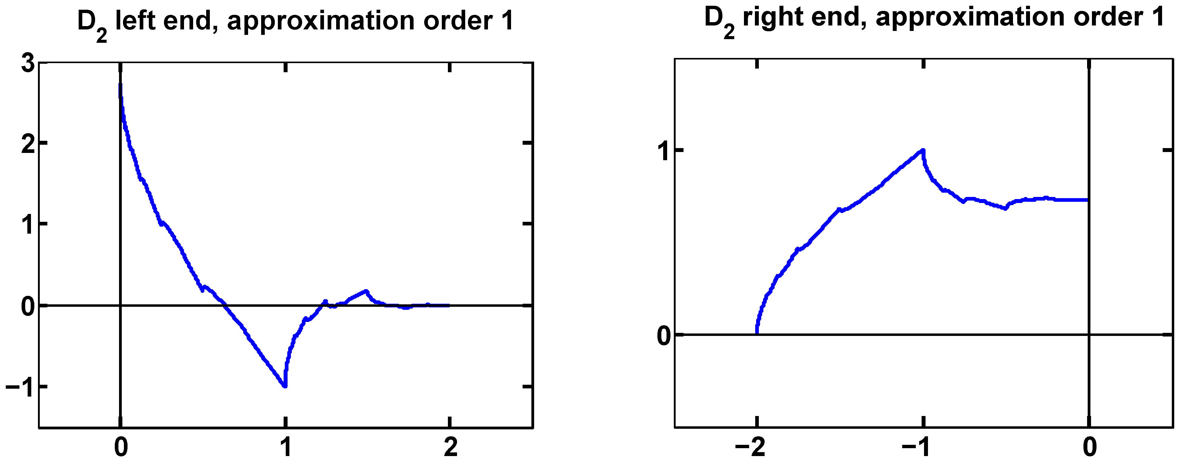
7.1. Example 1: Daubechies
As a very simple scalar example we consider the Daubechies scaling functions with two vanishing moments.
The recursion coefficients are
The approximation order is 2, but there is only a single boundary function at each end. We can impose approximation order 1 at each end.
At the left end, we find
At the right end, we get
These are the same boundary functions derived in [
8]. They are shown in
Figure 1.
Figure 1.
Boundary functions for with approximation order 1, at left and right ends.
Figure 1.
Boundary functions for with approximation order 1, at left and right ends.
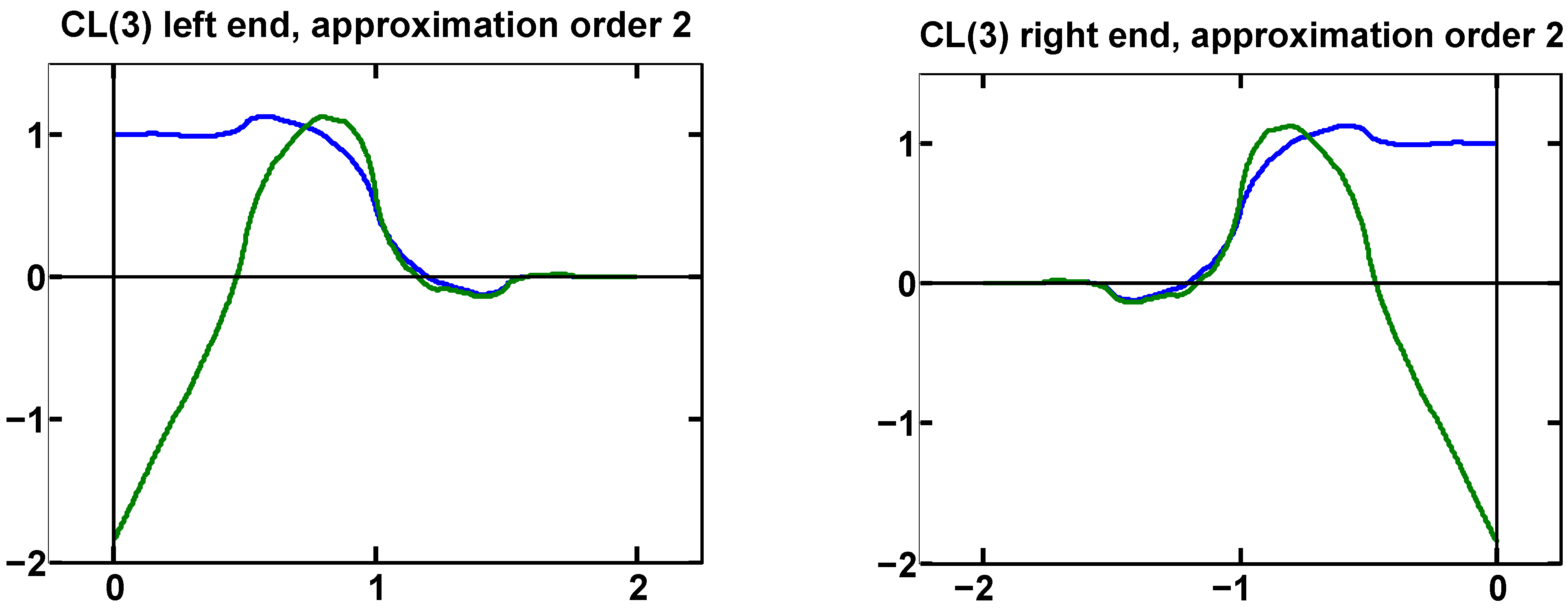
7.2. Example 2: CL(3) Multiwavelet
The Chui–Lian multiwavelet CL(3) [
16] has recursion coefficients
It has approximation order 3.
Here , so we need a vector of two boundary functions at each end. We can impose approximation order 2.
The original completion is
After applying the algorithm in
Section 6, we find that the top two rows of
must be
This leads to
Only the numerical approximations of
A,
B are shown, since the exact expressions get very messy.
This is the same solution found in [
8]. The boundary functions at the right end are the left end functions reversed, due to the symmetry of CL(3). The graphs are shown in
Figure 2.
Figure 2.
Boundary functions for CL(3) with approximation order 2, at left and right ends.
Figure 2.
Boundary functions for CL(3) with approximation order 2, at left and right ends.
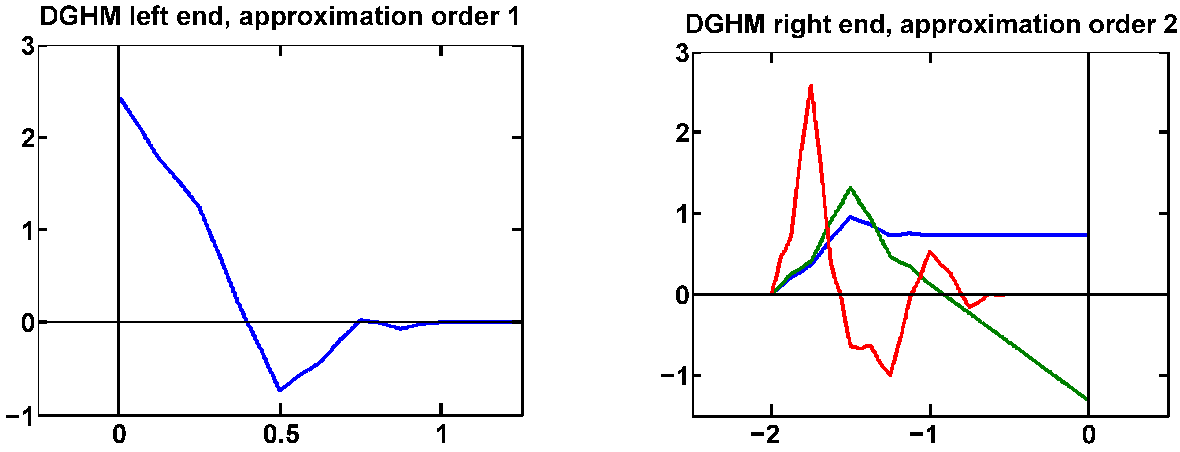
7.3. Example 3: DGHM Multiwavelet
The Donovan-Geronimo-Hardin-Massopust multiwavelet [
17] has approximation order 2 with recursion coefficients
Its support is
instead of the expected
, which causes some interesting effects.
We find , , so we have only a single boundary function at the left end, but three at the right end.
At the left end we can only enforce approximation order 1. The boundary scaling function found by our algorithm is the same one as in [
8].
At the right end we can enforce approximation order 2. This determines two of the boundary functions, corresponding to the orthonormalized combination of the first two basic solutions from [
8]. The third function (determined by the third row of
) is arbitrary, except that the diagonal entry in
Z should be smaller than
to ensure that the completion is regular.
As an example, we set the third column of
Z to zero, and let the QR-factorization built into MATLAB choose an appropriate third row of
Y. The result was
Figure 3.
Boundary functions for DGHM. The single left boundary function has approximation order 1. Three right boundary functions provide approximation order 2.
Figure 3.
Boundary functions for DGHM. The single left boundary function has approximation order 1. Three right boundary functions provide approximation order 2.
8. Summary
Boundary functions for wavelets on a finite interval can be constructed from linear combinations of boundary-crossing internal functions, or by finding recursion coefficients, or by linear algebra techniques. The problem with the linear algebra approach is that it involves multiplication by arbitrary orthogonal matrices. A random choice leads to boundary recursion coefficients that produce an invertible transform but do not correspond to any actual boundary functions. Also, these coefficients do not provide any approximation orders.
In this paper, we present a linear algebra algorithm that works for all multiwavelets and removes most or all of the non-uniqueness while ensuring maximum possible boundary approximation orders.


