Divergence-Free Multiwavelets on the Half Plane

Abstract

We use the biorthogonal multiwavelets related by differentiation constructed in previous work to construct compactly supported biorthogonal multiwavelet bases for the space of vector fields on the upper half plane ${\mathbb{R}}_{+}^2$ such that the reconstruction wavelets are divergence-free and have vanishing normal components on the boundary of ${\mathbb{R}}_{+}^2$. Such wavelets are suitable to study the Navier–Stokes equations on a half plane when imposing a Navier boundary condition.

1. Introduction

Wavelets have proved useful for the numerical analysis of an incompressible flow fluid that can be modeled by the Navier–Stokes equations. The incompressibility requires the wavelets to be divergence-free, at least in dimension three or greater.

Battle and Federbush [1] first constructed an orthogonal basis of divergence-free wavelets for the space of divergence-free vector fields on ${\mathbb{R}}^n$. The Battle–Federbush divergence-free wavelets are globally supported, and therefore unsuitable for numerical analysis on domains with boundary. It was shown by Lemarié that if a continuous divergence-free wavelet basis is orthogonal, the wavelets cannot be compactly supported [2]. Lemarié [3] also showed that this obstacle does not necessarily arise in the biorthogonal case. He used the existence of biorthogonal MRAs related by differentiation to construct compactly supported divergence-free wavelets. Lemarié’s method can be extended to higher dimensional spaces by using tensor products of univariate functions. His approach was then modified and extended in various works by Urban [4,5]. Those divergence-free wavelets have been used effectively for the numerical simulation of the Stokes equations on rectangular domains [6], and for the analysis of incompressible turbulent flows [7].

A velocity field $\overrightarrow{v}$ defined on a domain $\Omega \subset {\mathbb{R}}^2$ is said to satisfy Navier boundary conditions if $\overrightarrow{v}·\overrightarrow{n}=0$ and $2D\left(\overrightarrow{v}\right)\overrightarrow{n}·\overrightarrow{\tau }+\alpha \overrightarrow{v}·\overrightarrow{\tau }=0$ on $\partial \Omega$ where D denotes the strain tensor $D\left(v\right)=[\nabla \overrightarrow{v}+{\left(\nabla \overrightarrow{v}\right)}^T]/2$ and $\overrightarrow{n}$ and $\overrightarrow{\tau }$ are the unit normal and tangent vectors respectively. We will call the condition $\overrightarrow{v}·\overrightarrow{n}=0$ the vanishing normal boundary condition. When Ω is the upper half plane ${\mathbb{R}}_{+}^2$, $\overrightarrow{\tau }={\overrightarrow{e}}_1$ and $\overrightarrow{n}=-{\overrightarrow{e}}_2$ where ${\overrightarrow{e}}_1$ and ${\overrightarrow{e}}_2$ are the standard basis vectors. The study of the Navier–Stokes equations on half spaces with the Navier boundary condition remains a field of intensive research, e.g., [8]. Here we will adapt Lemarié’s technique to provide a construction for a multiwavelet basis of the divergence-free vector fields on the upper half plane ${\mathbb{R}}_{+}^2$ that satisfies the vanishing normal boundary condition using the biorthogonal multiwavelets on $\mathbb{R}$ introduced in [9]. This approach can easily be extended to higher dimensions, but we will work exclusively in ${\mathbb{R}}^2$ to minimize notational complexity.

Strela’s two-scale transform [10] plays a crucial role in extending Lemarié’s divergence-free construction to multiwavelets by providing certain commutation relations between oblique MRA projections and differentiation under suitable conditions on Strela’s transition matrix. To carry out the construction on the upper half plane ${\mathbb{R}}_{+}^2$, it is necessary that the wavelet bases of $L^2\left({\mathbb{R}}_{+}\right)$ adapted from those of $L^2\left(\mathbb{R}\right)$ are also related by differentiation and inherit the commutation relation between oblique projections and differentiation. These constraints plus the vanishing normal boundary conditions force the wavelet bases of $L^2\left(\mathbb{R}\right)$ to have an appropriate combination of biorthogonality, symmetry, regularity, support and boundary behavior. We will see that this can all be accomplished using the biorthogonal multiwavelet bases of $L^2\left(\mathbb{R}\right)$ constructed in [9].

2. Biorthogonal Multiwavelets of $L^2\left(\mathbb{R}\right)$

We review here in some detail the construction of biorthogonal multiwavelets related by differentiation introduced in [9]. The main tools for the construction are fractal interpolation functions [11] and Strela’s two-scale transform [10].

2.1. Some Preliminaries

Denote by $V_0=V(\Phi )$ the $L^2$-closure of the finite shift invariant space spanned by the integer translates $\{{\varphi }^i(·-k):i=0,\dots ,r-1;k\in \mathbb{Z}\}$ of ${\varphi }^1,\cdots ,{\varphi }^r,$ and let Φ denote the vector function $\Phi =({\varphi }^1,\cdots ,{\varphi }^r)$. It is standard to denote $V_j=\{f(2^j·):f\in V_0\}$. If $V_0\subset V_1$ then Φ is called a scaling vector. If, in addition, ${\cap }_{j\in \mathbb{Z}}{V}_j=\left\{0\right\}$, $\overline{{\cup }_{j\in \mathbb{Z}}{V}_j}=L^2\left(\mathbb{R}\right)$, and the integer shifts of ${\phi }_1,\cdots ,{\phi }_r$ form a Riesz basis for $V_0$, then the nested family ${\left\{V_j\right\}}_{j\in \mathbb{Z}}$ is called a multiresolution analysis of $L^2\left(\mathbb{R}\right)$ of multiplicity r.

The vector function $\Phi =({\varphi }^0,\dots ,{\varphi }^{r-1})$ is called a scaling vector and is said to generate the multiresolution analysis $\left\{V_j\right\}$. Φ satisfies a matrix–vector dilation equation

$$\Phi \left(x\right)=\frac{1}{2}\sum _{k\in \mathbb{Z}}{C}_k\Phi (2x-k)$$

(1)

for some sequence of $r\times r$ matrices $\left(C_k\right)$, called scaling coefficients.

We define the Fourier transform of a function $f\in L^1\left(\mathbb{R}\right)$ by

$$\widehat{f}\left(\omega \right)={\int }_{-\infty }^{\infty }f\left(t\right){\mathrm{e}}^{-\mathrm{i}t\omega }dt$$

Taking the Fourier transform of the dilation Equation (1), we obtain

$$\widehat{\Phi }\left(\omega \right)=H\left(\frac{\omega }{2}\right)\widehat{\Phi }\left(\frac{\omega }{2}\right);H\left(\omega \right)=\frac{1}{2}\sum _{k\in \mathbb{Z}}{C}_k{\mathrm{e}}^{-\mathrm{i}k\omega }$$

(2)

in which H is an $r\times r$ matrix of $2\pi$ periodic functions, called a scaling filter ; in addition $\widehat{\Phi }={\left[{\widehat{\varphi }}^0{\widehat{\varphi }}^1\dots {\widehat{\varphi }}^{r-1}\right]}^T$.

A vector function $\Psi =({\psi }^0,\dots ,{\psi }^{r-1})$ is called a multiwavelet associated with the scaling vector Φ if the integer translates $\{{\psi }^i(·-k):k\in \mathbb{Z}\}$ are linearly independent and

$$\{{\varphi }^i(·-k):i=0,\dots ,r-1;k\in \mathbb{Z}\}\cup \{{\psi }^i(·-k):i=0,\dots ,r-1;k\in \mathbb{Z}\}$$

is a Riesz basis of $V_1$. Let $W_j$ be the closed linear span of $\{{\psi }^i(2^j·-k):i=0,\dots ,r-1;k\in \mathbb{Z}\}$. Then

$$V_{j+1}=V_j\oplus W_j$$

where the symbol ⊕ denotes the internal direct sum, not necessarily orthogonal. The wavelet vector Ψ can be represented by the following equation

$$\Psi \left(x\right)=\frac{1}{2}\sum _{k\in \mathbb{Z}}{D}_k\Phi (2x-k)$$

(3)

for some sequence of $r\times r$ matrices $\left(D_k\right)$, called wavelet coefficients. In the Fourier domain,

$$\widehat{\Psi }\left(\omega \right)=F\left(\frac{\omega }{2}\right)\widehat{\Phi }\left(\frac{\omega }{2}\right),F\left(\omega \right)=\frac{1}{2}\sum _{k\in \mathbb{Z}}{D}_k{\mathrm{e}}^{-\mathrm{i}k\omega }$$

where F is an $r\times r$ matrix of $2\pi$ periodic functions, called a wavelet filter.

The scaling functions and wavelets will have finite support if and only if there are finitely many non-zero coefficients $C_k$ and $D_k$.

A multi scaling function $\Phi \left(t\right)$ is said to have approximation order m if each polynomial $t^j,j=0,\dots ,m-1,$ is a linear combination of integer translates $\Phi (t-k):$

$$t^j=\sum _{k\in \mathbb{Z}}{y}_k^{\left(j\right)}\Phi (t-k)\text{a.e.}$$

for $j=0,\dots ,m-1$, where the $y_k$’s are constant row-vectors of length r.

We say that a pair of vector functions $\Phi =({\varphi }^0,\dots ,{\varphi }^{r-1})$ and $\tilde{\Phi }=({\tilde{\varphi }}^0,\dots ,{\tilde{\varphi }}^{r-1})$ is biorthogonal if

$$⟨{\varphi }^i,{\tilde{\varphi }}^j(·-l)⟩={\delta }_{i,j}{\delta }_{0,l}$$

for all $i,j=0,\dots ,r-1$ and $l\in \mathbb{Z}$, where $⟨,⟩$ denotes the usual inner product in $L^2\left(\mathbb{R}\right)$. If the MRAs $\left\{V_j\right\}$ and $\left\{{\tilde{V}}_j\right\}$ are generated by the scaling vectors Φ and $\tilde{\Phi }$, respectively, then $\left\{V_j\right\}$ and $\left\{{\tilde{V}}_j\right\}$ are said to be a pair of biorthogonal MRAs if Φ and $\tilde{\Phi }$ are biorthogonal. If $\Psi =({\psi }^0,\dots ,{\psi }^{r-1})$ and $\tilde{\Psi }=({\tilde{\psi }}^0,\dots ,{\tilde{\psi }}^{r-1})$ are the multiwavelets associated with the scaling vectors Φ and $\tilde{\Phi }$ respectively, then Ψ and $\tilde{\Psi }$ are biorthogonal multiwavelets if

$$⟨{\varphi }^i,{\tilde{\psi }}^j(·-l)⟩=⟨{\tilde{\varphi }}^i,{\psi }^j(·-l)⟩=0\mathrm{and}⟨{\psi }^i,{\tilde{\psi }}^j(·-l)⟩={\delta }_{i,j}{\delta }_{0,l}$$

for $i,j=0,\dots ,r-1$ and $l\in \mathbb{Z}.$ In this case, $V_j\perp {\tilde{W}}_j$ and ${\tilde{V}}_j\perp W_j$. If $\Psi =({\psi }^0,\dots ,{\psi }^{r-1})$ and $\tilde{\Psi }=({\tilde{\psi }}^0,\dots ,{\tilde{\psi }}^{r-1})$ are biorthogonal multiwavelets then for $f\in L^2\left(\mathbb{R}\right)$,

$$f=\sum _{j,k\in \mathbb{Z};i=0}^{r-1}⟨f,{\psi }_{j,k}^i⟩{\tilde{\psi }}_{j,k}^i=\sum _{j,k\in \mathbb{Z};i=0}^{r-1}⟨f,{\tilde{\psi }}_{j,k}^i⟩{\psi }_{j,k}^i$$

2.2. Biorthogonal Multiwavelets from Fractal Interpolation

The parametric family of biorthogonal wavelets described here uses ideas similar to those developed by Massopust [12]. Let

$$u_0\left(x\right)=(1-x){\chi }_{[0,1]}\left(x\right),u_1\left(x\right)=x{\chi }_{[0,1]}\left(x\right),\mathrm{and}q\left(x\right)=u_0\left(x\right)u_1\left(x\right)$$

Fix $s\in (-1,1)$. The unique solution $w\left(x\right)=w_s$ of the inhomogeneous equation

$$w\left(x\right)=q\left(2x\right)-q(2x-1)+sw\left(2x\right)+sw(2x-1)$$

(4)

is called a fractal interpolation function. We will denote $\tilde{w}=w_{\tilde{s}}$ for a certain related value $\tilde{s}\in (-1,1)$. Define

$$v_i=u_i-\frac{⟨\tilde{w},u_i⟩w}{⟨w,\tilde{w}⟩}-\frac{⟨q,u_i⟩q}{⟨q,q⟩},i=0,1$$

and let ${\tilde{v}}_i$ be defined in the same way with w replaced by $\tilde{w}$. Set

$${\varphi }^0=\alpha q,{\varphi }^1=\beta w,{\varphi }^2=\left\{\begin{array}{ll}\gamma v_0& \text{if}x\in [0,1]\\ \gamma v_1(·+1)& \text{if}x\in [-1,0)\end{array}\right.$$

and define ${\tilde{\varphi }}^i$, $i=0,1,2$ in the same way with $v_i$ replaced by ${\tilde{v}}_i$ and the normalization parameters $\alpha ,\beta ,\gamma$ replaced by corresponding parameters $\tilde{\alpha },\tilde{\beta },\tilde{\gamma }$. Set $\Phi =({\varphi }^0,{\varphi }^1,{\varphi }^2)$ and

$$V_j={\text{cl}}_{L^2\left(\mathbb{R}\right)}\text{span}\{{\varphi }^i(2^j·-k):i=0,1,2;j,k\in \mathbb{Z}\}$$

and define $\tilde{\Phi }$ and ${\tilde{V}}_j$ similarly. We proved in [9] that

Theorem 2.1. For $-\frac{1}{2}<\tilde{s}<0$ and $s=\frac{1+2\tilde{s}}{2(3\tilde{s}-1)}$,

1. 

$\left\{V_j\right\}$ and $\left\{{\tilde{V}}_j\right\}$ form a pair of biorthogonal MRAs of $L^2\left(\mathbb{R}\right)$.

2. 

Φ and $\tilde{\Phi }$ are piecewise $C^1$ biorthogonal multiscaling functions. Their components ${\varphi }^0$, ${\tilde{\varphi }}^0$ are supported on $[0,1]$ and symmetric about $1/2$; ${\varphi }^1$, ${\tilde{\varphi }}^1$ are supported on $[0,1]$ and antisymmetric about $1/2$; ${\varphi }^2$, ${\tilde{\varphi }}^2$ are supported on $[-1,1]$ and symmetric about 0.

3. 

Φ and $\tilde{\Phi }$ have approximation order 3.

Let H and $\tilde{H}$ be the scaling filter of Φ and $\tilde{\Phi }$, respectively. As in [9], to construct biorthogonal multiwavelets related by differentiation via Strela’s two-scale transform, one needs $H\left(0\right)$ and $\tilde{H}\left(0\right)$ to be symmetric. For this reason, we chose $\alpha =\tilde{\alpha }=\sqrt{30}$, $\beta =\tilde{\beta }=\sqrt{260/9}$, $\gamma =\tilde{\gamma }=\sqrt{6}$.

The biorthogonal scaling vectors Φ and $\tilde{\Phi }$ are represented by the scaling equations

$$\Phi \left(x\right)=\frac{1}{2}\sum _{k=-2}^1{C}_k\Phi (2x-k),\tilde{\Phi }\left(x\right)=\frac{1}{2}\sum _{k=-2}^1{\tilde{C}}_k\tilde{\Phi }(2x-k)$$

(5)

The biorthogonal multiwavelets $\Psi =({\psi }^0,{\psi }^1,{\psi }^2)$ and $\tilde{\Psi }=({\tilde{\psi }}^0,{\tilde{\psi }}^1,{\tilde{\psi }}^2)$ associated with the respective scaling vectors Φ and $\tilde{\Phi }$ are represented by corresponding equations

$$\Psi \left(x\right)=\frac{1}{2}\sum _{k=-2}^1{D}_k\Phi (2x-k),\tilde{\Psi }\left(x\right)=\frac{1}{2}\sum _{k=-2}^1{\tilde{D}}_k\tilde{\Phi }(2x-k)$$

(6)

With appropriate choice of coefficients the multiwavelets are also supported on $[-1,1]$ and possess corresponding symmetry properties. The scaling coefficients and wavelet coefficients for the parameter choices $s=-1/6$, $\tilde{s}=-2/9$ can be found in Appendix A. The components of the scaling and wavelet vectors are plotted in Figure 1.

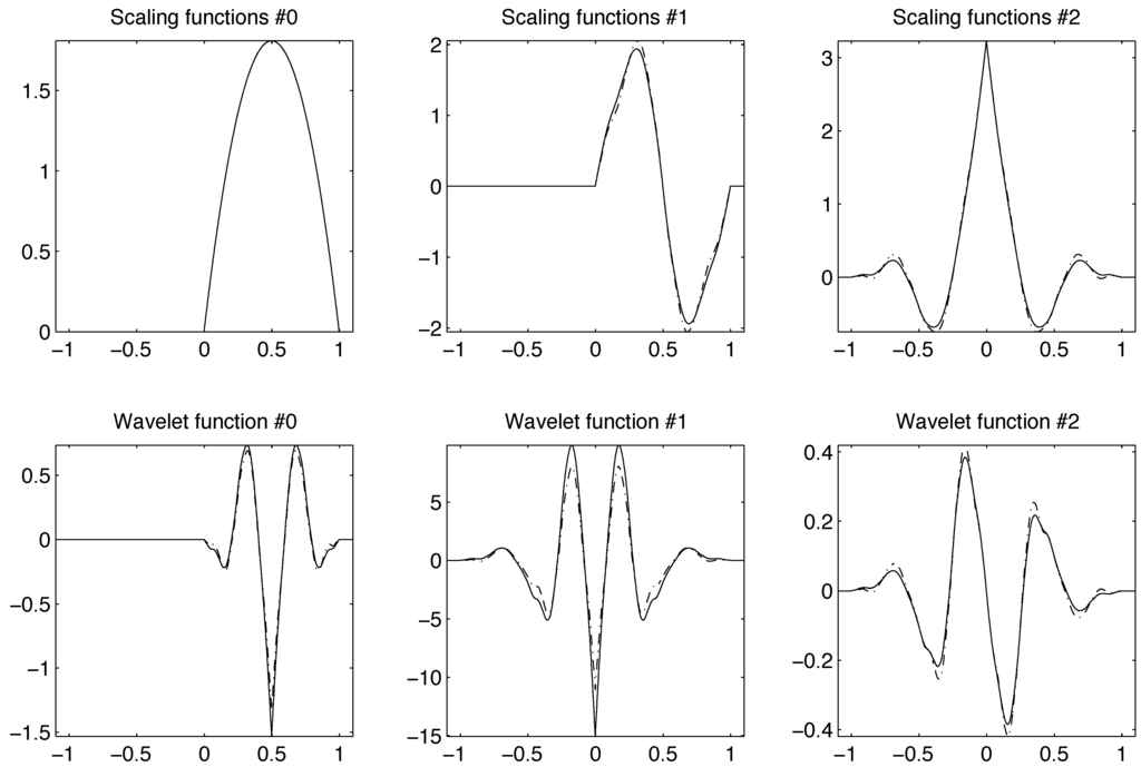
Figure 1. Scaling vectors Φ (solid) and $\tilde{\Phi }$ (dashed) and multiwavelets Ψ and $\tilde{\Psi }$, $s=-1/6$.

Figure 1. Scaling vectors Φ (solid) and $\tilde{\Phi }$ (dashed) and multiwavelets Ψ and $\tilde{\Psi }$, $s=-1/6$.

2.3. Biorthogonal Multiwavelets via Strela’s Two-Scale Transform

Strela’s two-scale transform is a method to derive a new scaling filter from a given scaling filter by a transform $H^{\mathrm{old}}\left(\omega \right)\mapsto H^{\mathrm{new}}\left(\omega \right)=\frac{1}{2}M\left(2\omega \right)H^{\mathrm{old}}\left(\omega \right)M^{-1}\left(\omega \right)$ in which the relative properties of $H^{\mathrm{old}}$ and $H^{\mathrm{new}}$ are encoded in the transition matrix M. Strela proved that if $detM$ is linear in ${\mathrm{e}}^{\mathrm{i}\omega }$ with a unique zero at $\omega =0$ and if the kernel of $M\left(0\right)$ is the 1-eigenvector of $H^{\mathrm{old}}\left(0\right)$ then the scaling vector of $H^{\mathrm{new}}$ will have one more order of approximation and regularity than $H^{\mathrm{old}}$ has. Using Strela’s two-scale transform [10], we obtained in [9] new biorthogonal multiwavelets related by differentiation to the ones we constructed from fractal interpolation functions, as explained below.

2.3.1. Smoothing Procedure

The transition matrix and two-scale transform filter

$${\tilde{H}}^{+}\left(\omega \right)=\frac{1}{2}M\left(2\omega \right)\tilde{H}\left(\omega \right)M^{-1}\left(\omega \right);M=\left[\begin{array}{ccc}1+{\mathrm{e}}^{\mathrm{i}\omega }& 0& -2\sqrt{5}\\ 0& 1& 0\\ 1-{\mathrm{e}}^{\mathrm{i}\omega }& 0& 0\end{array}\right]$$

(7)

have the properties just indicated. ${\tilde{H}}^{+}\left(\omega \right)$ then is the filter of a new scaling vector ${\tilde{\Phi }}^{+}$ having one more approximation order and regularity than the original scaling vector $\tilde{\Phi }$ whose components appear in Figure 1. By Theorem 2.1, ${\tilde{\Phi }}^{+}$ is piecewise $C^2$ and has approximation order 4. One associates to ${\tilde{\Phi }}^{+}$ the multiwavelet vector ${\tilde{\Psi }}^{+}$ defined by the filter ${\tilde{F}}^{+}$ defined by (see Lakey and Pereyra [13])

$$\widehat{{\tilde{\Psi }}^{+}}\left(\omega \right)=F^{+}\left(\frac{\omega }{2}\right)\widehat{{\tilde{\Phi }}^{+}}\left(\frac{\omega }{2}\right);F^{+}\left(\omega \right)=-\frac{1}{2}\tilde{F}\left(\omega \right)M^{-1}\left(\omega \right)$$

(8)

where $\tilde{F}$ is the filter of the multiwavelet $\tilde{\Psi }$ derived from Equation (6).

The transition matrix M induces an operator symbol matrix

$$T_M=\left[\begin{array}{ccc}I+S^{-1}& 0& -2\sqrt{5}I\\ 0& I& 0\\ I-S^{-1}& 0& 0\end{array}\right]$$

(9)

Here I denotes the identity operator and S is the shift operator $Sf=f(·-1)$, so $S^{-1}f=f(·+1)$. We proved in [9] that the smoothed scaling vector and the associated multiwavelet are related to the original ones by the following differentiation relations

$$D{\tilde{\Phi }}^{+}=T_M\tilde{\Phi },D{\tilde{\Psi }}^{+}=-\tilde{\Psi }$$

(10)

where $Df$ denotes the distributional derivative of f. The components ${\tilde{\varphi }}^{i,+}$ and ${\tilde{\psi }}^{i,+}$, $i=0,1,2$ of ${\tilde{\Phi }}^{+}$ and ${\tilde{\Psi }}^{+}$ satisfy the following.

Theorem 2.2. [9] Let ${\tilde{\Phi }}^{+}$ and ${\tilde{\Psi }}^{+}$ be defined as above. Then

1. 

The components of ${\tilde{\Phi }}^{+}$ and ${\tilde{\Psi }}^{+}$ are piecewise $C^2$ and have approximation order 4.

2. 

${\tilde{\varphi }}^{0,+}$ is supported on $[-1,1]$ and antisymmetric about 0; ${\tilde{\varphi }}^{1,+}$ is supported on $[0,1]$ and symmetric about $1/2$; ${\tilde{\varphi }}^{2,+}$ is supported on $[-1,1]$ and symmetric about 0.

3. 

${\tilde{\psi }}^{0,+}$ is supported on $[0,1]$ and antisymmetric about $1/2$; ${\tilde{\psi }}^{1,+}$ is supported on $[-1,1]$ and antisymmetric about 0; ${\tilde{\psi }}^{2,+}$ is supported on $[-1,1]$ and symmetric about 0.

The smoothed scaling and wavelet filter matrices have the form

$${\tilde{H}}^{+}\left(\omega \right)=\frac{1}{2}\sum _{k=-2}^1{\tilde{C}}_k^{+}{\mathrm{e}}^{-\mathrm{i}k\omega }\mathrm{and}{\tilde{F}}^{+}\left(\omega \right)=\frac{1}{2}\sum _{k=-2}^1{\tilde{D}}_k^{+}{\mathrm{e}}^{-\mathrm{i}k\omega }$$

(11)

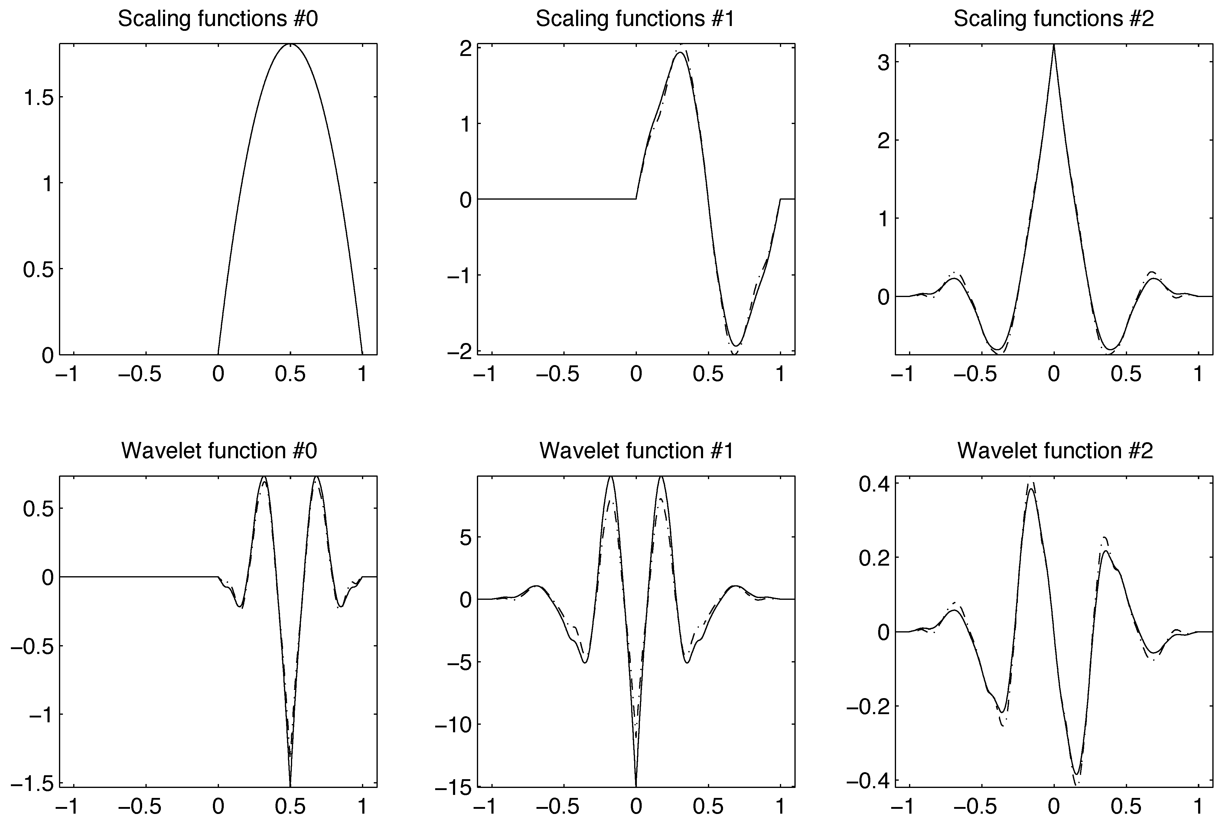
with values determined by Equations (7) and (8). The matrices $C_k^{+}$ and $D_k^{+}$ corresponding to the parameter choices $s=-1/6$, $\tilde{s}=-2/9$ are given in Appendix A. The components of the smoothed scaling and wavelet vectors are plotted in Figure 2.

Figure 2. Smoothed scaling vector ${\tilde{\Phi }}^{+}$ and multiwavelet ${\tilde{\Psi }}^{+}$.

Figure 2. Smoothed scaling vector ${\tilde{\Phi }}^{+}$ and multiwavelet ${\tilde{\Psi }}^{+}$.

2.3.2. Roughening Procedure

Following Strela, the scaling vector ${\Phi }^{-}$ of the filter $H^{-}$ defined by

$$H^{-}\left(\omega \right)=2N^{-1}\left(2\omega \right)H\left(\omega \right)N\left(\omega \right);N\left(\omega \right)=-M^{*}\left(\omega \right)=\left[\begin{array}{ccc}-1-{\mathrm{e}}^{-\mathrm{i}\omega }& 0& -1+{\mathrm{e}}^{-\mathrm{i}\omega }\\ 0& -1& 0\\ 2\sqrt{5}& 0& 0\end{array}\right]$$

(12)

has one less approximation order and regularity than the old scaling vector Φ. Hence, ${\Phi }^{-}$ is piecewise continuous and of approximation order 2. An associated multiwavelet ${\Psi }^{-}$ can be defined by (see Lakey and Pereyra [13])

$$\widehat{{\Psi }^{-}}\left(\omega \right)=F^{-}\left(\frac{\omega }{2}\right)\widehat{{\Phi }^{-}}\left(\frac{\omega }{2}\right);F^{-}\left(\omega \right)=2F\left(\omega \right)N\left(\omega \right)$$

(13)

It can also be verified that, with $T_N$ the symbol matrix corresponding to N as in Equation (9), the roughened and original scaling vectors and multiwavelets are related by

$$D\Phi =T_N{\Phi }^{-},D\Psi ={\Psi }^{-}$$

(14)

Denote by ${\varphi }^{i,-}$ and ${\psi }^{i,-}$, $i=0,1,2$ the components of ${\Phi }^{-}$ and ${\Psi }^{-}$ respectively.

Theorem 2.3. [9] Let ${\Phi }^{-}$, ${\tilde{\Phi }}^{+}$, ${\Psi }^{-}$ and ${\tilde{\Psi }}^{+}$ be defined as above. Then, in the exact order given, a component of ${\Phi }^{-}$ or ${\Psi }^{-}$ and the corresponding component of ${\tilde{\Phi }}^{+}$ or ${\tilde{\Psi }}^{+}$ have the same support and symmetry. In addition,

$${\varphi }^{0,-}{\chi }_{[0,1]}={\varphi }^{2,-}{\chi }_{[0,1]}\text{and}{\varphi }^{0,-}{\chi }_{[-1,0]}=-{\varphi }^{2,-}{\chi }_{[-1,0]}$$

The values of the coefficients $C_k^{-}$ and $D_k^{-}$ of the roughened scaling and wavelet filters

$$H^{-}\left(\omega \right)=\frac{1}{2}\sum _{k=-2}^2{C}_k^{-}{\mathrm{e}}^{-\mathrm{i}k\omega }\mathrm{and}{F}^{-}\left(\omega \right)=\frac{1}{2}\sum _{k=-2}^2{D}_k^{-}{\mathrm{e}}^{-\mathrm{i}k\omega }$$

(15)

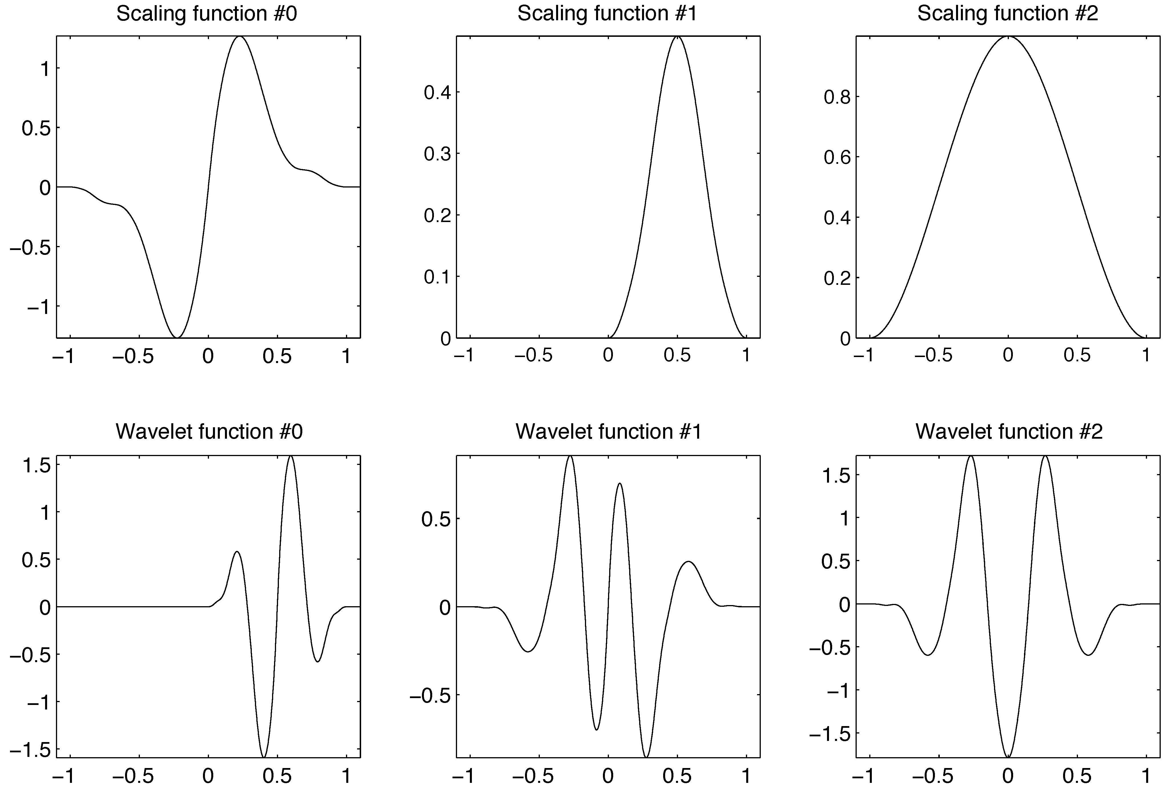
with the same parameter values $s=-1/6$, $\tilde{s}=-2/9$ are determined by Equations (12) and (13) and are given in Appendix A. The components of the roughened scaling and wavelet vectors are plotted in Figure 3.

Figure 3. Roughened scaling vector ${\Phi }^{-}$ and multiwavelet ${\Psi }^{-}$.

Figure 3. Roughened scaling vector ${\Phi }^{-}$ and multiwavelet ${\Psi }^{-}$.

Theorem 2.4. [9] The scaling vectors ${\tilde{\Phi }}^{+}$ and ${\Phi }^{-}$ generate a pair of biorthogonal MRAs of $L^2\left(\mathbb{R}\right)$. In addition, ${\tilde{\Psi }}^{+}$ and ${\Psi }^{-}$ are biorthogonal multiwavelets.

The old and new biorthogonal multiwavelet bases of $L^2\left(\mathbb{R}\right)$ satisfy commutation relations between oblique MRA projections and differentiation. The commutation relations are crucial in the construction of divergence-free wavelets on ${\mathbb{R}}_{+}^2$.

Denote the oblique projections ${\tilde{P}}_j$ and ${\tilde{P}}_j^{+}$ from $L^2\left(\mathbb{R}\right)$ onto the respective approximation spaces ${\tilde{V}}_j$ and ${\tilde{V}}_j^{+}$ by

$${\tilde{P}}_{j}f=\sum _{i,k}⟨f,{\varphi }_{j,k}^i⟩{\tilde{\varphi }}_{j,k}^i,{\tilde{P}}_j^{+}f=\sum _{i,k}⟨f,{\varphi }_{j,k}^{i,-}⟩{\tilde{\varphi }}_{j,k}^{i,+}$$

(16)

Define the oblique projections ${\tilde{Q}}_j$ and ${\tilde{Q}}_j^{+}$ from $L^2\left(\mathbb{R}\right)$ onto the corresponding detail spaces ${\tilde{W}}_j$ and ${\tilde{W}}_j^{+}$ similarly,

$${\tilde{Q}}_{j}f=\sum _{i,k}⟨f,{\psi }_{j,k}^i⟩{\tilde{\psi }}_{j,k}^i,{\tilde{Q}}_j^{+}f=\sum _{i,k}⟨f,{\psi }_{j,k}^{i,-}⟩{\tilde{\psi }}_{j,k}^{i,+}$$

(17)

Notice that for a fixed value $x\in \mathbb{R}$, the sums in Equations (16) and (17) are finite sums with respect to k due to the finiteness of the support of the scaling and wavelet functions.

Proposition 2.1. [9] For $f\in H^1\left(\mathbb{R}\right)$, the following commutation relations hold

$${\tilde{P}}_{j}D=D{\tilde{P}}_j^{+},{\tilde{Q}}_{j}D=D{\tilde{Q}}_j^{+}$$

3. Divergence-Free Multiwavelets on ${\mathbb{R}}_{+}^2$

To construct divergence-free multiwavelets on the upper half plane ${\mathbb{R}}_{+}^2$, we first need to adapt the biorthogonal multiwavelets related by differentiation on $\mathbb{R}$ to the half line ${\mathbb{R}}_{+}$.

3.1. Biorthogonal Multiwavelet Bases of $L^2\left({\mathbb{R}}_{+}\right)$

We construct a pair of biorthogonal multiwavelet bases of $L^2\left({\mathbb{R}}_{+}\right)$ using the original multiwavelet systems $(\Phi ,\Psi )$, $(\tilde{\Phi },\tilde{\Psi })$ and the derived systems $({\tilde{\Phi }}^{+},{\tilde{\Psi }}^{+})$, $({\Phi }^{-},{\Psi }^{-})$ of $L^2\left(\mathbb{R}\right)$. Divergence-free wavelets satisfying vanishing normal boundary conditions can then be constructed through tensor products from a basis of $L^2\left({\mathbb{R}}_{+}\right)$ generated from the smoothed multiwavelet system $({\tilde{\Phi }}^{+},{\tilde{\Psi }}^{+})$ vanishing on the boundary of its support.

Our procedure for constructing biorthogonal multiwavelet bases of $L^2\left({\mathbb{R}}_{+}\right)$ adapted from those of $L^2\left(\mathbb{R}\right)$ can be described as follows:

• Keep the functions that are originally supported on $[0,\infty )$,
• For the functions belonging to the original biorthogonal systems of $L^2\left(\mathbb{R}\right)$ whose support straddles the boundary point 0, truncate the symmetric ones to $[0,\infty )$ and normalize them by $\sqrt{2}$, and shift the antisymmetric ones to $[0,\infty )$.
• For the functions belonging to the smoothed and roughened systems of $L^2\left(\mathbb{R}\right)$ whose support straddles the boundary point 0, truncate the antisymmetric ones to $[0,\infty )$ and normalize them by $\sqrt{2}$, and shift the symmetric ones to $[0,\infty )$.

Precisely, for $j,k\ge 0$, we define

$${\varphi }_{{\mathbb{R}}_{+},j,k}^i={\varphi }_{j,k}^i\text{if}i=0,1,{\varphi }_{{\mathbb{R}}_{+},j,k}^2=\left\{\begin{array}{cc}\sqrt{2}{\varphi }_{j,k}^2{\chi }_{[0,\infty )}\hfill & \text{if}k=0\hfill \\ {\varphi }_{j,k}^2\hfill & \text{if}k\ge 1\hfill \end{array}\right.$$

(18)

and

$${\psi }_{{\mathbb{R}}_{+},j,k}^i=\left\{\begin{array}{cc}{\psi }_{j,k}^i\hfill & \text{if}i=0\hfill \\ {\psi }_{j,k+1}^i\hfill & \text{if}i=2,\hfill \end{array}\right.{\psi }_{{\mathbb{R}}_{+},j,k}^1=\left\{\begin{array}{cc}\sqrt{2}{\psi }_{j,k}^1{\chi }_{[0,\infty )}\hfill & \text{if}k=0\hfill \\ {\psi }_{j,k}^1\hfill & \text{if}k\ge 1\hfill \end{array}\right.$$

(19)

Use the same formulation for ${\tilde{\varphi }}_{{\mathbb{R}}_{+},j,k}^i$ and ${\tilde{\psi }}_{{\mathbb{R}}_{+},j,k}^i$. Let

$$V_j\left({\mathbb{R}}_{+}\right)={\text{cl}}_{L^2\left({\mathbb{R}}_{+}\right)}\text{span}\{{\varphi }_{{\mathbb{R}}_{+},j,k}^i:i=0,1,2;j,k\ge 0\}$$

$$W_j\left({\mathbb{R}}_{+}\right)={\text{cl}}_{L^2\left({\mathbb{R}}_{+}\right)}\text{span}\{{\psi }_{{\mathbb{R}}_{+},j,k}^i:i=0,1,2;j,k\ge 0\}$$

and similarly for ${\tilde{V}}_j\left({\mathbb{R}}_{+}\right),{\tilde{W}}_j\left({\mathbb{R}}_{+}\right)$ in terms of ${\tilde{\varphi }}_{{\mathbb{R}}_{+},j,k}^i,{\tilde{\psi }}_{{\mathbb{R}}_{+},j,k}^i$, respectively. We obtain a pair of biorthogonal MRAs $\left\{V_j\left({\mathbb{R}}_{+}\right)\right\}$ and $\left\{{\tilde{V}}_j\left({\mathbb{R}}_{+}\right)\right\}$ of $L^2\left({\mathbb{R}}_{+}\right)$ such that

$$V_{j+1}\left({\mathbb{R}}_{+}\right)=V_j\left({\mathbb{R}}_{+}\right)\oplus W_j\left({\mathbb{R}}_{+}\right),{\tilde{V}}_{j+1}\left({\mathbb{R}}_{+}\right)={\tilde{V}}_j\left({\mathbb{R}}_{+}\right)\oplus {\tilde{W}}_j\left({\mathbb{R}}_{+}\right)$$

and , just as in the case of the whole real line,

$$L^2\left({\mathbb{R}}_{+}\right)=V_0\left({\mathbb{R}}_{+}\right)\underset{j\ge 0}{⨁}{W}_j\left({\mathbb{R}}_{+}\right)={\tilde{V}}_0\left({\mathbb{R}}_{+}\right)\underset{j\ge 0}{⨁}{\tilde{W}}_j\left({\mathbb{R}}_{+}\right)$$

We perform a similar procedure for the construction of the biorthogonal multiwavelet bases of $L^2\left({\mathbb{R}}_{+}\right)$ generated from the new systems $({\tilde{\Phi }}^{+},{\tilde{\Psi }}^{+})$ and $({\Phi }^{-},{\Psi }^{-})$ of $L^2\left(\mathbb{R}\right)$ except that the roles of symmetric and antisymmetric components whose support overlaps 0 are switched. Explicitly, for $j,k\ge 0$, let

$${\tilde{\varphi }}_{{\mathbb{R}}_{+},j,k}^{i,+}=\left\{\begin{array}{cc}{\tilde{\varphi }}_{j,k}^{i,+}\hfill & \text{if}i=1\hfill \\ {\tilde{\varphi }}_{j,k+1}^{i,+}\hfill & \text{if}i=2,\hfill \end{array}\right.{\tilde{\varphi }}_{{\mathbb{R}}_{+},j,k}^{0,+}=\left\{\begin{array}{cc}\sqrt{2}{\tilde{\varphi }}_{j,k}^{0,+}{\chi }_{[0,\infty )}\hfill & \text{if}k=0\hfill \\ {\tilde{\varphi }}_{j,k}^{0,+}\hfill & \text{if}k\ge 1\hfill \end{array}\right.$$

(20)

and

$${\tilde{\psi }}_{{\mathbb{R}}_{+},j,k}^{i,+}=\left\{\begin{array}{cc}{\tilde{\psi }}_{j,k}^{i,+}\hfill & \text{if}i=0\hfill \\ {\tilde{\psi }}_{j,k+1}^{i,+}\hfill & \text{if}i=2,\hfill \end{array}\right.{\tilde{\psi }}_{{\mathbb{R}}_{+},j,k}^{1,+}=\left\{\begin{array}{cc}\sqrt{2}{\tilde{\psi }}_{j,k}^{1,+}{\chi }_{[0,\infty )}\hfill & \text{if}k=0\hfill \\ {\tilde{\psi }}_{j,k}^{1,+}\hfill & \text{if}k\ge 1\hfill \end{array}\right.$$

(21)

We define similarly for ${\varphi }_{{\mathbb{R}}_{+},j,k}^{i,-}$ and ${\psi }_{{\mathbb{R}}_{+},j,k}^{i,-}$. Let

$${\tilde{V}}_j^{+}\left({\mathbb{R}}_{+}\right)={\text{cl}}_{L^2\left({\mathbb{R}}_{+}\right)}\text{span}\{{\tilde{\varphi }}_{{\mathbb{R}}_{+},j,k}^{i,+}:i=0,1,2;j,k\ge 0\}$$

$${\tilde{W}}_j^{+}\left({\mathbb{R}}_{+}\right)={\text{cl}}_{L^2\left({\mathbb{R}}_{+}\right)}\text{span}\{{\tilde{\psi }}_{{\mathbb{R}}_{+},j,k}^{i,+}:i=0,1,2;j,k\ge 0\}$$

and similarly for $V_j^{-}\left({\mathbb{R}}_{+}\right),W_j^{-}\left({\mathbb{R}}_{+}\right)$ in terms of ${\varphi }_{{\mathbb{R}}_{+},j,k}^{i,-},{\psi }_{{\mathbb{R}}_{+},j,k}^{i,-}$, respectively. We get another pair of biorthogonal MRAs $\left\{{\tilde{V}}_j^{+}\left({\mathbb{R}}_{+}\right)\right\}$ and $\left\{V_j^{-}\left({\mathbb{R}}_{+}\right)\right\}$ of $L^2\left({\mathbb{R}}_{+}\right)$ such that

$${\tilde{V}}_{j+1}^{+}\left({\mathbb{R}}_{+}\right)={\tilde{V}}_j^{+}\left({\mathbb{R}}_{+}\right)\oplus {\tilde{W}}_j^{+}\left({\mathbb{R}}_{+}\right),V_{j+1}^{-}\left({\mathbb{R}}_{+}\right)=V_j^{-}\left({\mathbb{R}}_{+}\right)\oplus W_j^{-}\left({\mathbb{R}}_{+}\right)$$

and

$$L^2\left({\mathbb{R}}_{+}\right)={\tilde{V}}_0^{+}\left({\mathbb{R}}_{+}\right)\underset{j\ge 0}{⨁}{\tilde{W}}_j^{+}\left({\mathbb{R}}_{+}\right)=V_0^{-}\left({\mathbb{R}}_{+}\right)\underset{j\ge 0}{⨁}{W}_j^{-}\left({\mathbb{R}}_{+}\right)$$

To adapt the differentiation and integration relations between the scaling vectors and multiwavelets on $\mathbb{R}$ to ones on ${\mathbb{R}}_{+}$, we separate the scaling vectors and multiwavelets on ${\mathbb{R}}_{+}$ into boundary and interior components. We define the boundary scaling vectors and multiwavelets, which correspond to the integer translate $k=0$, as follows

$$\begin{array}{cc}\hfill {\Phi }_{{\mathbb{R}}_{+}}^0& ={\left[{\varphi }_{{\mathbb{R}}_{+}}^0{\varphi }_{{\mathbb{R}}_{+}}^1{\varphi }_{{\mathbb{R}}_{+}}^2\right]}^T={\left[{\varphi }^0{\varphi }^1\sqrt{2}{\varphi }^2{\chi }_{[0,\infty )}\right]}^T\hfill \\ \hfill {\Psi }_{{\mathbb{R}}_{+}}^0& ={\left[{\psi }_{{\mathbb{R}}_{+}}^0{\psi }_{{\mathbb{R}}_{+}}^1{\psi }_{{\mathbb{R}}_{+}}^2\right]}^T={\left[{\psi }^0\sqrt{2}{\psi }^1{\chi }_{[0,\infty )}{\psi }^2(·-1)\right]}^T\hfill \\ \hfill {\tilde{\Phi }}_{{\mathbb{R}}_{+}}^{0,+}& ={\left[{\tilde{\varphi }}_{{\mathbb{R}}_{+}}^{0,+}{\tilde{\varphi }}_{{\mathbb{R}}_{+}}^{1,+}{\tilde{\varphi }}_{{\mathbb{R}}_{+}}^{2,+}\right]}^T={\left[\sqrt{2}{\tilde{\varphi }}^{0,+}{\chi }_{[0,\infty )}{\tilde{\varphi }}^{1,+}{\tilde{\varphi }}^{2,+}(·-1)\right]}^T\hfill \\ \hfill {\tilde{\Psi }}_{{\mathbb{R}}_{+}}^{0,+}& ={\left[{\tilde{\psi }}_{{\mathbb{R}}_{+}}^{0,+}{\tilde{\psi }}_{{\mathbb{R}}_{+}}^{1,+}{\tilde{\psi }}_{{\mathbb{R}}_{+}}^{2,+}\right]}^T={\left[{\tilde{\psi }}^{0,+}\sqrt{2}{\tilde{\psi }}^{1,+}{\chi }_{[0,\infty )}{\tilde{\psi }}^{2,+}(·-1)\right]}^T\hfill \end{array}$$

We define ${\tilde{\Phi }}_{{\mathbb{R}}_{+}}^0,{\tilde{\Psi }}_{{\mathbb{R}}_{+}}^0,{\Phi }_{{\mathbb{R}}_{+}}^{0,-}$ and ${\Psi }_{{\mathbb{R}}_{+}}^{0,-}$ similarly to ${\Phi }_{{\mathbb{R}}_{+}}^0,{\Psi }_{{\mathbb{R}}_{+}}^0,{\tilde{\Phi }}_{{\mathbb{R}}_{+}}^{0,+}$ and ${\tilde{\Psi }}_{{\mathbb{R}}_{+}}^{0,+}$, respectively. The interior components, formulated as below, are the scaling vectors and multiwavelets on ${\mathbb{R}}_{+}$ with the integer translates $k\ge 1$, which live completely inside $[0,\infty )$. Let

$$\begin{array}{cc}\hfill {\Phi }_{{\mathbb{R}}_{+}}^k& ={\left[{\varphi }_{{\mathbb{R}}_{+},0,k}^0{\varphi }_{{\mathbb{R}}_{+},0,k}^1{\varphi }_{{\mathbb{R}}_{+},0,k}^2\right]}^T={\left[{\varphi }_{0,k}^0{\varphi }_{0,k}^1{\varphi }_{0,k}^2\right]}^T\hfill \\ \hfill {\Psi }_{{\mathbb{R}}_{+}}^k& ={\left[{\psi }_{{\mathbb{R}}_{+},0,k}^0{\psi }_{{\mathbb{R}}_{+},0,k}^1{\psi }_{{\mathbb{R}}_{+},0,k}^2\right]}^T={\left[{\psi }_{0,k}^0{\psi }_{0,k}^1{\psi }_{0,k+1}^2\right]}^T\hfill \\ \hfill {\tilde{\Phi }}_{{\mathbb{R}}_{+}}^{k,+}& ={\left[{\tilde{\varphi }}_{{\mathbb{R}}_{+},0,k}^{0,+}{\tilde{\varphi }}_{{\mathbb{R}}_{+},0,k}^{1,+}{\tilde{\varphi }}_{{\mathbb{R}}_{+},0,k}^{2,+}\right]}^T={\left[{\tilde{\varphi }}_{0,k}^{0,+}{\tilde{\varphi }}_{0,k}^{1,+}{\tilde{\varphi }}_{0,k+1}^{2,+}\right]}^T\hfill \\ \hfill {\tilde{\Psi }}_{{\mathbb{R}}_{+}}^{k,+}& ={\left[{\tilde{\psi }}_{{\mathbb{R}}_{+},0,k}^{0,+}{\tilde{\psi }}_{{\mathbb{R}}_{+},0,k}^{1,+}{\tilde{\psi }}_{{\mathbb{R}}_{+},0,k}^{2,+}\right]}^T={\left[{\tilde{\psi }}_{0,k}^{0,+}{\tilde{\psi }}_{0,k}^{1,+}{\tilde{\psi }}_{0,k+1}^{2,+}\right]}^T\hfill \end{array}$$

and similarly for ${\tilde{\Phi }}_{{\mathbb{R}}_{+}}^k,{\tilde{\Psi }}_{{\mathbb{R}}_{+}}^k,{\Phi }_{{\mathbb{R}}_{+}}^{k,-}$ and ${\Psi }_{{\mathbb{R}}_{+}}^{k,-}$.

From Equations (10) and (14), and Equations (19) and (21) the multiwavelets on ${\mathbb{R}}_{+}$ inherit the same differentiation and integration relations as the multiwavelets on $\mathbb{R}$. Precisely,

$$D{\tilde{\Psi }}_{{\mathbb{R}}_{+}}^{k,+}=-{\tilde{\Psi }}_{{\mathbb{R}}_{+}}^k,D{\Psi }_{{\mathbb{R}}_{+}}^k={\Psi }_{{\mathbb{R}}_{+}}^{k,-}$$

(22)

for both interior and boundary components $k=0$ and $k\ge 1$.

The boundary and interior scaling vectors on ${\mathbb{R}}_{+}$ are less straightforward. From Equations (9) and (10) and Equations (18) and (20) that define the scaling functions on ${\mathbb{R}}_{+}$ we obtain

$$D{\tilde{\Phi }}_{{\mathbb{R}}_{+}}^{0,+}=T_{M_{\partial }}{\tilde{\Phi }}_{{\mathbb{R}}_{+}}^0\mathrm{and}D{\tilde{\Phi }}_{{\mathbb{R}}_{+}}^{k,+}=T_{M_{\text{int}}}{\tilde{\Phi }}_{{\mathbb{R}}_{+}}^k(k\ge 1)$$

(23)

for the respective boundary and interior scaling vectors, where

$$T_{M_{\partial }}:=\left[\begin{array}{ccc}\sqrt{2}I& 0& -2\sqrt{5}I\\ 0& I& 0\\ S-I& 0& 0\end{array}\right]\mathrm{and}{T}_{M_{\text{int}}}:=\left[\begin{array}{ccc}I+S^{-1}& 0& -2\sqrt{5}I\\ 0& I& 0\\ S-I& 0& 0\end{array}\right]$$

To establish an analogue of Proposition 2.1 on ${\mathbb{R}}_{+}$, we define oblique projections ${\tilde{P}}_{{\mathbb{R}}_{+},j}$, ${\tilde{P}}_{{\mathbb{R}}_{+},j}^{+}$ from $L^2\left({\mathbb{R}}_{+}\right)$ onto the respective approximation spaces ${\tilde{V}}_j\left({\mathbb{R}}_{+}\right)$ and ${\tilde{V}}_j^{+}\left({\mathbb{R}}_{+}\right)$ and ${\tilde{Q}}_{{\mathbb{R}}_{+},j}$, ${\tilde{Q}}_{{\mathbb{R}}_{+},j}^{+}$ from $L^2\left({\mathbb{R}}_{+}\right)$ onto the corresponding detail spaces ${\tilde{W}}_j\left({\mathbb{R}}_{+}\right)$ and ${\tilde{W}}_j^{+}\left({\mathbb{R}}_{+}\right)$ as follows:

$$\begin{array}{ccc}\hfill {\tilde{P}}_{{\mathbb{R}}_{+},j}f& =& \sum _{i,k}⟨f,{\varphi }_{{\mathbb{R}}_{+},j,k}^i⟩{\tilde{\varphi }}_{{\mathbb{R}}_{+},j,k}^i,{\tilde{P}}_{{\mathbb{R}}_{+},j}^{+}f=\sum _{i,k}⟨f,{\varphi }_{{\mathbb{R}}_{+},j,k}^{i,-}⟩{\tilde{\varphi }}_{{\mathbb{R}}_{+},j,k}^{i,+}\hfill \\ \hfill {\tilde{Q}}_{{\mathbb{R}}_{+},j}f& =& \sum _{i,k}⟨f,{\psi }_{{\mathbb{R}}_{+},j,k}^i⟩{\tilde{\psi }}_{{\mathbb{R}}_{+},j,k}^i,{\tilde{Q}}_{{\mathbb{R}}_{+},j}^{+}f=\sum _{i,k}⟨f,{\psi }_{{\mathbb{R}}_{+},j,k}^{i,-}⟩{\tilde{\psi }}_{{\mathbb{R}}_{+},j,k}^{i,+}\hfill \end{array}$$

For an interval $\Omega \subset \mathbb{R}$, possibly unbounded, the Sobolev space $H^1(\Omega )$ is the Hilbert space defined by

$$H^1(\Omega )=\{f\in L^2(\Omega ):Df\in L^2(\Omega )\}{,\parallel f\parallel }_{H^1(\Omega )}^2={\parallel f\parallel }_{L^2(\Omega )}^2+{\parallel Df\parallel }_{L^2(\Omega )}^2$$

Define

$$H_0^1(\Omega )={\text{cl}}_{H^1(\Omega )}{C}_c^1(\Omega )(={\text{cl}}_{H^1(\Omega )}{C}_c^{\infty }(\Omega ))$$

where $C_c^1(\Omega )$ is the space of continuously differentiable functions compactly supported in Ω. Note that if $f\in H^1(\Omega )$ then $f\in H_0^1(\Omega )$ if and only if $Df=0$ on $\partial \Omega$ .

Proposition 3.1. On the Sobolev space $H_0^1\left({\mathbb{R}}_{+}\right)$, the following commutation relations hold

$${\tilde{P}}_{{\mathbb{R}}_{+},j}D=D{\tilde{P}}_{{\mathbb{R}}_{+},j}^{+},{\tilde{Q}}_{{\mathbb{R}}_{+},j}D=D{\tilde{Q}}_{{\mathbb{R}}_{+},j}^{+}$$

The proof of Proposition 3.1 can be found in Appendix B.

3.2. Construction of Divergence-Free Multiwavelets

The following are some basic notions of flux spaces and divergence-free vector fields. Denote

$${\mathbb{R}}_{+}^2=\{(x,y)\in {\mathbb{R}}^2:y\ge 0\}$$

the upper half plane, and

$$L^2{\left({\mathbb{R}}_{+}^2\right)}^2=\{\overrightarrow{F}=(F_1,F_2):F_i\in L^2\left({\mathbb{R}}_{+}^2\right),i=1,2\}$$

The divergence operator $\nabla :L^2{\left({\mathbb{R}}_{+}^2\right)}^2\to L^2\left({\mathbb{R}}_{+}^2\right)$ is defined as usual by

$$\nabla \overrightarrow{F}=\frac{\partial F_1}{\partial x}+\frac{\partial F_2}{\partial y}$$

where the partial derivatives are understood in the distributional sense. The divergence operator induces the flux space

$$H(\text{div},{\mathbb{R}}_{+}^2)=\{\overrightarrow{F}\in L^2{\left({\mathbb{R}}_{+}^2\right)}^2:\nabla \overrightarrow{F}\in L^2\left({\mathbb{R}}_{+}^2\right)\}$$

and its divergence-free subspace

$$H^0(\text{div},{\mathbb{R}}_{+}^2)=\{\overrightarrow{F}\in H(\text{div},{\mathbb{R}}_{+}^2):\nabla \overrightarrow{F}=0\}$$

The two spaces of vector fields are Hilbert spaces under the norm

$${\parallel \overrightarrow{F}\parallel }_{H(\text{div},{\mathbb{R}}_{+}^2)}^2={\parallel \overrightarrow{F}\parallel }_{L^2{\left({\mathbb{R}}_{+}^2\right)}^2}^2+{\parallel \nabla \overrightarrow{F}\parallel }_{L^2\left({\mathbb{R}}_{+}^2\right)}^2$$

where

$${\parallel \overrightarrow{F}\parallel }_{L^2{\left({\mathbb{R}}_{+}^2\right)}^2}^2=\sum _{i=1}^2{\parallel F_i\parallel }_{L^2\left({\mathbb{R}}_{+}^2\right)}^2$$

We have found biorthogonal multiwavelet systems related by differentiation for both $L^2\left(\mathbb{R}\right)$ and $L^2\left({\mathbb{R}}_{+}\right)$ so that the commutation relations between oblique projections and differentiation are all satisfied. We are now able to construct a wavelet basis for the vector space $H^0(\text{div},{\mathbb{R}}_{+}^2)$ satisfying the vanishing normal boundary condition $\overrightarrow{v}·\overrightarrow{n}=0$, where $\overrightarrow{n}=-{\overrightarrow{e}}_2$ is the unit outward normal vector to the boundary axis $\left\{\right(x,0):x\in \mathbb{R}\}$.

We have utilized many notations so far. To avoid confusion, we recall the notations and relations that are necessary for the construction.

• Biorthogonal scaling vectors $(\Phi ,\tilde{\Phi })$ and $({\tilde{\Phi }}^{+},{\Phi }^{-})$ and wavelets $(\Psi ,\tilde{\Psi })$ and $({\tilde{\Psi }}^{+},{\Psi }^{-})$ on $\mathbb{R}$, related by Equation (10).
• Biorthogonal boundary scaling vectors $({\Phi }_{{\mathbb{R}}_{+}}^0,{\tilde{\Phi }}_{{\mathbb{R}}_{+}}^0)$ and $({\tilde{\Phi }}_{{\mathbb{R}}_{+}}^{0,+},{\Phi }_{{\mathbb{R}}_{+}}^{0,-})$ and wavelets $({\Psi }_{{\mathbb{R}}_{+}}^0,{\tilde{\Psi }}_{{\mathbb{R}}_{+}}^0)$ and $({\tilde{\Psi }}_{{\mathbb{R}}_{+}}^{0,+},{\Psi }_{{\mathbb{R}}_{+}}^{0,-})$ on ${\mathbb{R}}_{+}$, related by related by Equations (22) and (23).
• Biorthogonal interior scaling vectors $({\Phi }_{{\mathbb{R}}_{+}}^k,{\tilde{\Phi }}_{{\mathbb{R}}_{+}}^k)$ and $({\tilde{\Phi }}_{{\mathbb{R}}_{+}}^{k,+},{\Phi }_{{\mathbb{R}}_{+}}^{k,-})$ and wavelets $({\Psi }_{{\mathbb{R}}_{+}}^k,{\tilde{\Psi }}_{{\mathbb{R}}_{+}}^k)$ and $({\tilde{\Psi }}_{{\mathbb{R}}_{+}}^{k,+},{\Psi }_{{\mathbb{R}}_{+}}^{k,-})$, $k\ge 1$ on ${\mathbb{R}}_{+}$, related by Equations (22) and (23). These multiwavelet systems establish the commutation relations as in Propositions 2.1 and 3.1.

Our construction of biorthogonal bases of compactly supported multiwavelets on ${\mathbb{R}}_{+}^2$ such that the reconstruction wavelets are divergence-free will be divided into the following steps.

Step 1. Compose biorthogonal multiwavelet bases in $L^2\left({\mathbb{R}}_{+}^2\right)$ by tensor products.

We use the standard basis vectors ${\overrightarrow{e}}_1=(1,0)$ and ${\overrightarrow{e}}_2=(0,1)$ to index a smoothing direction for tensor wavelets on ${\mathbb{R}}_{+}^2$:

$$\begin{array}{cc}\hfill V_j^{{\overrightarrow{e}}_1}\left({\mathbb{R}}_{+}^2\right)& =V_j^{(1,0)}\left({\mathbb{R}}_{+}^2\right)={\tilde{V}}_j^{+}\left(\mathbb{R}\right)\otimes {\tilde{V}}_j\left({\mathbb{R}}_{+}\right)\hfill \\ \hfill V_j^{{\overrightarrow{e}}_2}\left({\mathbb{R}}_{+}^2\right)& =V_j^{(0,1)}\left({\mathbb{R}}_{+}^2\right)={\tilde{V}}_j\left(\mathbb{R}\right)\otimes {\tilde{V}}_j^{+}\left({\mathbb{R}}_{+}\right)\hfill \\ \hfill W_j^{{\overrightarrow{e}}_1}\left({\mathbb{R}}_{+}^2\right)& =[{\tilde{V}}_j^{+}\left(\mathbb{R}\right)\otimes {\tilde{W}}_j\left({\mathbb{R}}_{+}\right)]\oplus [{\tilde{W}}_j^{+}\left(\mathbb{R}\right)\otimes {\tilde{V}}_j\left({\mathbb{R}}_{+}\right)]\oplus [{\tilde{W}}_j^{+}\left(\mathbb{R}\right)\otimes {\tilde{W}}_j\left({\mathbb{R}}_{+}\right)]\hfill \\ \hfill W_j^{{\overrightarrow{e}}_2}\left({\mathbb{R}}_{+}^2\right)& =[{\tilde{V}}_j\left(\mathbb{R}\right)\otimes {\tilde{W}}_j^{+}\left({\mathbb{R}}_{+}\right)]\oplus [{\tilde{W}}_j\left(\mathbb{R}\right)\otimes {\tilde{V}}_j^{+}\left({\mathbb{R}}_{+}\right)]\oplus [{\tilde{W}}_j\left(\mathbb{R}\right)\otimes {\tilde{W}}_j^{+}\left({\mathbb{R}}_{+}\right)]\hfill \end{array}$$

Then

$$L^2\left({\mathbb{R}}_{+}^2\right)=V_0^{(1,0)}\left({\mathbb{R}}_{+}^2\right)\underset{j\ge 0}{⨁}{W}_j^{(1,0)}\left({\mathbb{R}}_{+}^2\right)=V_0^{(0,1)}\left({\mathbb{R}}_{+}^2\right)\underset{j\ge 0}{⨁}{W}_j^{(0,1)}\left({\mathbb{R}}_{+}^2\right)$$

(24)

Similarly, we use negated standard basis vectors to index roughening directions for dual tensor scaling and wavelet spaces on ${\mathbb{R}}_{+}^2$:

$$\begin{array}{cc}\hfill V_j^{-{\overrightarrow{e}}_1}\left({\mathbb{R}}_{+}^2\right)& =V_j^{(-1,0)}\left({\mathbb{R}}_{+}^2\right)=V_j^{-}\left(\mathbb{R}\right)\otimes V_j\left({\mathbb{R}}_{+}\right)\hfill \\ \hfill V_j^{-{\overrightarrow{e}}_2}\left({\mathbb{R}}_{+}^2\right)& =V_j^{(0,-1)}\left({\mathbb{R}}_{+}^2\right)=V_j\left(\mathbb{R}\right)\otimes V_j^{-}\left({\mathbb{R}}_{+}\right)\hfill \end{array}$$

$$\begin{array}{cc}\hfill W_j^{-{\overrightarrow{e}}_1}\left({\mathbb{R}}_{+}^2\right)& =[V_j^{-}\left(\mathbb{R}\right)\otimes W_j\left({\mathbb{R}}_{+}\right)]\oplus [W_j^{-}\left(\mathbb{R}\right)\otimes V_j\left({\mathbb{R}}_{+}\right)]\oplus [W_j^{-}\left(\mathbb{R}\right)\otimes W_j\left({\mathbb{R}}_{+}\right)]\hfill \\ \hfill W_j^{-{\overrightarrow{e}}_2}\left({\mathbb{R}}_{+}^2\right)& =[V_j\left(\mathbb{R}\right)\otimes W_j^{-}\left({\mathbb{R}}_{+}\right)]\oplus [W_j\left(\mathbb{R}\right)\otimes V_j^{-}\left({\mathbb{R}}_{+}\right)]\oplus [W_j\left(\mathbb{R}\right)\otimes W_j^{-}\left({\mathbb{R}}_{+}\right)]\hfill \end{array}$$

The decomposition corresponding to Equation (24) holds for the respective indices $-{\overrightarrow{e}}_1$ and $-{\overrightarrow{e}}_2$.

We define the boundary generators of $L^2\left({\mathbb{R}}_{+}^2\right)$ to be components of the matrices

$$\begin{array}{cc}\hfill {\Gamma }_{\partial ,1}^{{\overrightarrow{e}}_1}(x,y)& ={\Gamma }_{\partial ,1}^{(1,0)}(x,y)={\tilde{\Psi }}^{+}{\left(x\right)}^T{\tilde{\Psi }}_{{\mathbb{R}}_{+}}^0\left(y\right);{\Gamma }_{\partial ,1}^{-{\overrightarrow{e}}_1}(x,y)={\Gamma }_{\partial ,1}^{(-1,0)}(x,y)={\Psi }^{-}{\left(x\right)}^T{\Psi }_{{\mathbb{R}}_{+}}^0\left(y\right)\hfill \\ \hfill {\Gamma }_{\partial ,2}^{{\overrightarrow{e}}_1}(x,y)& ={\Gamma }_{\partial ,2}^{(1,0)}(x,y)={\tilde{\Psi }}^{+}{\left(x\right)}^T{\tilde{\Phi }}_{{\mathbb{R}}_{+}}^0\left(y\right);{\Gamma }_{\partial ,2}^{-{\overrightarrow{e}}_1}(x,y)={\Gamma }_{\partial ,2}^{(-1,0)}(x,y)={\Psi }^{-}{\left(x\right)}^T{\Phi }_{{\mathbb{R}}_{+}}^0\left(y\right)\hfill \\ \hfill {\Gamma }_{\partial ,3}^{{\overrightarrow{e}}_1}(x,y)& ={\Gamma }_{\partial ,3}^{(1,0)}(x,y)={\tilde{\Phi }}^{+}{\left(x\right)}^T{\tilde{\Psi }}_{{\mathbb{R}}_{+}}^0\left(y\right);{\Gamma }_{\partial ,3}^{-{\overrightarrow{e}}_1}(x,y)={\Gamma }_{\partial ,3}^{(-1,0)}(x,y)={\Phi }^{-}{\left(x\right)}^T{\Psi }_{{\mathbb{R}}_{+}}^0\left(y\right)\hfill \end{array}$$

Here ${\Gamma }_{\partial ,\mu }^{-{\overrightarrow{e}}_1}$ is biorthogonal to ${\Gamma }_{\partial ,\nu }^{{\overrightarrow{e}}_1}$, that is, $\int \int {\Gamma }_{\partial ,\mu }^{-{\overrightarrow{e}}_1}{\left({\Gamma }^{{\overrightarrow{e}}_1}\right)}_{\partial ,\nu }^T={\delta }_{\mu ,\nu }I$. We have another set of boundary biorthogonal generators of $L^2\left({\mathbb{R}}_{+}^2\right)$ given by

$$\begin{array}{cc}\hfill {\Gamma }_{\partial ,1}^{{\overrightarrow{e}}_2}(x,y)& ={\Gamma }_{\partial ,1}^{(0,1)}(x,y)=\tilde{\Psi }{\left(x\right)}^T{\tilde{\Psi }}_{{\mathbb{R}}_{+}}^{0,+}\left(y\right);{\Gamma }_{\partial ,1}^{-{\overrightarrow{e}}_2}(x,y)={\Gamma }_{\partial ,1}^{(0,-1)}(x,y)=\Psi {\left(x\right)}^T{\Psi }_{{\mathbb{R}}_{+}}^{0,-}\left(y\right)\hfill \\ \hfill {\Gamma }_{\partial ,2}^{{\overrightarrow{e}}_2}(x,y)& ={\Gamma }_{\partial ,2}^{(0,1)}(x,y)=\tilde{\Psi }{\left(x\right)}^T{\tilde{\Phi }}_{{\mathbb{R}}_{+}}^{0,+}\left(y\right);{\Gamma }_{\partial ,2}^{-{\overrightarrow{e}}_2}(x,y)={\Gamma }_{\partial ,2}^{(0,-1)}(x,y)=\Psi {\left(x\right)}^T{\Phi }_{{\mathbb{R}}_{+}}^{0,-}\left(y\right)\hfill \\ \hfill {\Gamma }_{\partial ,3}^{{\overrightarrow{e}}_2}(x,y)& ={\Gamma }_{\partial ,3}^{(0,1)}(x,y)=\tilde{\Phi }{\left(x\right)}^T{\tilde{\Psi }}_{{\mathbb{R}}_{+}}^{0,+}\left(y\right);{\Gamma }_{\partial ,3}^{-{\overrightarrow{e}}_2}(x,y)={\Gamma }_{\partial ,3}^{(0,-1)}(x,y)=\Phi {\left(x\right)}^T{\Psi }_{{\mathbb{R}}_{+}}^{0,-}\left(y\right)\hfill \end{array}$$

We define similarly biorthogonal interior generators of $L^2\left({\mathbb{R}}_{+}^2\right)$: $({\Gamma }_{\text{int},\ell }^{{\overrightarrow{e}}_1}, {\Gamma }_{\text{int},\ell }^{-{\overrightarrow{e}}_1})$ and $({\Gamma }_{\text{int},\ell }^{{\overrightarrow{e}}_2}, {\Gamma }_{\text{int},\ell }^{-{\overrightarrow{e}}_2})$, $\ell =1,2,3$, where each boundary scaling vector or multiwavelet is replaced by the corresponding interior one. For instance,

$${\Gamma }_{\text{int},1}^{{\overrightarrow{e}}_1}(x,y)={\Gamma }_{\text{int},1}^{(1,0)}(x,y)={\tilde{\Psi }}^{+}{\left(x\right)}^T{\tilde{\Psi }}_{{\mathbb{R}}_{+}}^1\left(y\right)$$

Along with the boundary generators, they constitute two biorthogonal bases of $L^2\left({\mathbb{R}}_{+}^2\right)$ as listed below:

• ${\Gamma }_{\partial ,\ell }^{{\overrightarrow{e}}_1},{\Gamma }_{\text{int},\ell }^{{\overrightarrow{e}}_1}$ with the duals ${\Gamma }_{\partial ,\ell }^{-{\overrightarrow{e}}_1},{\Gamma }_{\text{int},\ell }^{-{\overrightarrow{e}}_1}$; $\ell =1,2,3$
• ${\Gamma }_{\partial ,\ell }^{{\overrightarrow{e}}_2},{\Gamma }_{\text{int},\ell }^{{\overrightarrow{e}}_2}$ with the duals ${\Gamma }_{\partial ,\ell }^{-{\overrightarrow{e}}_2},{\Gamma }_{\text{int},\ell }^{-{\overrightarrow{e}}_2}$; $\ell =1,2,3$.

Step 2. Compose biorthogonal bases of $L^2{\left({\mathbb{R}}_{+}^2\right)}^2$ componentwise.

The biorthogonal bases of $L^2\left({\mathbb{R}}_{+}^2\right)$ induce biorthogonal bases of $L^2{\left({\mathbb{R}}_{+}^2\right)}^2$ componentwise. In fact, ${\{{\Gamma }_{\partial ,\ell }^{{\overrightarrow{e}}_1}{\overrightarrow{e}}_1,{\Gamma }_{\text{int},\ell }^{{\overrightarrow{e}}_1}{\overrightarrow{e}}_1,{\Gamma }_{\partial ,\ell }^{{\overrightarrow{e}}_2}{\overrightarrow{e}}_2,{\Gamma }_{\text{int},\ell }^{{\overrightarrow{e}}_2}{\overrightarrow{e}}_2\}}_{\ell =1,2,3}$ with the dual components $\{{\Gamma }_{\partial ,\ell }^{-{\overrightarrow{e}}_1}{\overrightarrow{e}}_1, {\Gamma }_{\text{int},\ell }^{-{\overrightarrow{e}}_1}{\overrightarrow{e}}_1, {\Gamma }_{\partial ,\ell }^{-{\overrightarrow{e}}_2}{\overrightarrow{e}}_2, {\Gamma }_{\text{int},\ell }^{-{\overrightarrow{e}}_2}{\overrightarrow{e}}_2{\}}_{\ell =1,2,3}$ form biorthogonal bases of $L^2{\left({\mathbb{R}}_{+}^2\right)}^2$. The following is the list of the boundary matrix generators. The interior generators and their duals are formulated similarly using the appropriate substitution of the boundary vector by the interior vector. Explicitly,

$$\begin{array}{cc}\hfill {\Gamma }_{\partial ,1}^{{\overrightarrow{e}}_1}(x,y){\overrightarrow{e}}_1& =\left({\tilde{\Psi }}^{+}{\left(x\right)}^T{\tilde{\Psi }}_{{\mathbb{R}}_{+}}^0\left(y\right),0\right);{\Gamma }_{\partial ,1}^{-{\overrightarrow{e}}_1}(x,y){\overrightarrow{e}}_1=\left({\Psi }^{-}{\left(x\right)}^T{\Psi }_{{\mathbb{R}}_{+}}^0\left(y\right),0\right)\hfill \\ \hfill {\Gamma }_{\partial ,2}^{{\overrightarrow{e}}_1}(x,y){\overrightarrow{e}}_1& =\left({\tilde{\Psi }}^{+}{\left(x\right)}^T{\tilde{\Phi }}_{{\mathbb{R}}_{+}}^0\left(y\right),0\right);{\Gamma }_{\partial ,2}^{-{\overrightarrow{e}}_1}(x,y){\overrightarrow{e}}_1=\left({\Psi }^{-}{\left(x\right)}^T{\Phi }_{{\mathbb{R}}_{+}}^0\left(y\right),0\right)\hfill \\ \hfill {\Gamma }_{\partial ,3}^{{\overrightarrow{e}}_1}(x,y){\overrightarrow{e}}_1& =\left({\tilde{\Phi }}^{+}{\left(x\right)}^T{\tilde{\Psi }}_{{\mathbb{R}}_{+}}^0\left(y\right),0\right);{\Gamma }_{\partial ,3}^{-{\overrightarrow{e}}_1}(x,y){\overrightarrow{e}}_1=\left({\Phi }^{-}{\left(x\right)}^T{\Psi }_{{\mathbb{R}}_{+}}^0\left(y\right),0\right)\hfill \\ \hfill {\Gamma }_{\partial ,1}^{{\overrightarrow{e}}_2}(x,y){\overrightarrow{e}}_2& =\left(0,\tilde{\Psi }{\left(x\right)}^T{\tilde{\Psi }}_{{\mathbb{R}}_{+}}^{0,+}\left(y\right)\right);{\Gamma }_{\partial ,1}^{-{\overrightarrow{e}}_2}(x,y){\overrightarrow{e}}_2=\left(0,\Psi {\left(x\right)}^T{\Psi }_{{\mathbb{R}}_{+}}^{0,-}\left(y\right)\right)\hfill \\ \hfill {\Gamma }_{\partial ,2}^{{\overrightarrow{e}}_2}(x,y){\overrightarrow{e}}_2& =\left(0,\tilde{\Psi }{\left(x\right)}^T{\tilde{\Phi }}_{{\mathbb{R}}_{+}}^{0,+}\left(y\right)\right);{\Gamma }_{\partial ,2}^{-{\overrightarrow{e}}_2}(x,y){\overrightarrow{e}}_2=\left(0,\Psi {\left(x\right)}^T{\Phi }_{{\mathbb{R}}_{+}}^{0,-}\left(y\right)\right)\hfill \\ \hfill {\Gamma }_{\partial ,3}^{{\overrightarrow{e}}_2}(x,y){\overrightarrow{e}}_2& =\left(0,\tilde{\Phi }{\left(x\right)}^T{\tilde{\Psi }}_{{\mathbb{R}}_{+}}^{0,+}\left(y\right)\right);{\Gamma }_{\partial ,3}^{-{\overrightarrow{e}}_2}(x,y){\overrightarrow{e}}_2=\left(0,\Phi {\left(x\right)}^T{\Psi }_{{\mathbb{R}}_{+}}^{0,-}\left(y\right)\right)\hfill \end{array}$$

Step 3. Compose the biorthogonal bases in $H^0(div,{\mathbb{R}}_{+}^2)$.

We can obtain a biorthogonal basis in $H^0(\text{div},{\mathbb{R}}_{+}^2)$ from the linear combinations of the vector fields listed above and their integer translates. The following are the reconstruction boundary multiwavelets of the basis:

$$\begin{array}{cc}\hfill {\overrightarrow{\tilde{\Psi }}}_{\partial ,1}(x,y)& =\left({\tilde{\Psi }}^{+}{\left(x\right)}^T{\tilde{\Psi }}_{{\mathbb{R}}_{+}}^0\left(y\right),-\tilde{\Psi }{\left(x\right)}^T{\tilde{\Psi }}_{{\mathbb{R}}_{+}}^{0,+}\left(y\right)\right)\hfill \\ \hfill {\overrightarrow{\tilde{\Psi }}}_{\partial ,2}(x,y)& =\left({\tilde{\Psi }}^{+}{\left(x\right)}^T{T}_{M_{\partial }}{\tilde{\Phi }}_{{\mathbb{R}}_{+}}^0\left(y\right),\tilde{\Psi }{\left(x\right)}^T{\tilde{\Phi }}_{{\mathbb{R}}_{+}}^{0,+}\left(y\right)\right)\hfill \\ \hfill {\overrightarrow{\tilde{\Psi }}}_{\partial ,3}(x,y)& =\left({\tilde{\Phi }}^{+}{\left(x\right)}^T{\tilde{\Psi }}_{{\mathbb{R}}_{+}}^0\left(y\right),T_{M_{\partial }}\tilde{\Phi }{\left(x\right)}^T{\tilde{\Psi }}_{{\mathbb{R}}_{+}}^{0,+}\left(y\right)\right)\hfill \end{array}$$

Because each component of ${\tilde{\Phi }}_{{\mathbb{R}}_{+}}^{0,+}$ and of ${\tilde{\Psi }}_{{\mathbb{R}}_{+}}^{0,+}$ vanishes continuously at $y=0$, these boundary multiwavelets satisfy the vanishing normal condition, that is, their normal component vanishes continuously at the boundary.

We formulate the reconstruction interior multiwavelets ${\overrightarrow{\tilde{\Psi }}}_{\text{int},\ell },\ell =1,2,3$ similarly, where $T_{M_{\partial }}$ and the boundary component are substituted respectively by $T_{M_{\text{int}}}$ and the corresponding interior component. For instance,

$${\overrightarrow{\tilde{\Psi }}}_{\text{int},2}(x,y)=\left({\tilde{\Psi }}^{+}{\left(x\right)}^T{T}_{M_{\text{int}}}{\tilde{\Phi }}_{{\mathbb{R}}_{+}}^1\left(y\right),\tilde{\Psi }{\left(x\right)}^T{\tilde{\Phi }}_{{\mathbb{R}}_{+}}^{1,+}\left(y\right)\right)$$

The vectors ${\overrightarrow{\tilde{\Psi }}}_{\partial ,\ell }$ and ${\overrightarrow{\tilde{\Psi }}}_{\text{int},\ell }$, $\ell =1,2,3,$ belong to the divergence-free vector space $H^0(\text{div},{\mathbb{R}}_{+}^2)$ because of the commutation relations between oblique projections and differentiation on both $\mathbb{R}$ and ${\mathbb{R}}_{+}$ specified by Propositions 2.1 and 3.1. We prove below that the reconstruction wavelets ${\overrightarrow{\tilde{\Psi }}}_{\partial ,\ell }$ and ${\overrightarrow{\tilde{\Psi }}}_{\text{int},\ell }$, $\ell =1,2,3,$ constitute a basis for $H^0(\text{div},{\mathbb{R}}_{+}^2)$. Their biorthogonal duals, which serve as the decomposition wavelets, are

$$\begin{array}{cc}\hfill {\overrightarrow{\Psi }}_{\partial ,1}(x,y)& =\left({\Psi }^{-}{\left(x\right)}^T{\Psi }_{{\mathbb{R}}_{+}}^0\left(y\right),0\right)\hfill \\ \hfill {\overrightarrow{\Psi }}_{\partial ,2}(x,y)& =\left(0,\Psi {\left(x\right)}^T{\Phi }_{{\mathbb{R}}_{+}}^{0,-}\left(y\right)\right)\hfill \\ \hfill {\overrightarrow{\Psi }}_{\partial ,3}(x,y)& =\left({\Phi }^{-}{\left(x\right)}^T{\Psi }_{{\mathbb{R}}_{+}}^0\left(y\right),0\right)\hfill \end{array}$$

for the boundary components. The interior components ${\overrightarrow{\Psi }}_{\text{int},\ell },\ell =1,2,3,$ are defined similarly. For instance

$${\overrightarrow{\Psi }}_{\text{int},1}(x,y)=\left({\Psi }^{-}{\left(x\right)}^T{\Psi }_{{\mathbb{R}}_{+}}^1\left(y\right),0\right)$$

Notice that the decomposition multiwavelets are not divergence-free.

Theorem 3.1. For $F\in H^0(div,{\mathbb{R}}_{+}^2)$, the expansion of F in terms of $\{({\Gamma }_{\partial ,\ell }^{{\overrightarrow{e}}_p}·{\overrightarrow{e}}_p,{\Gamma }_{int,\ell }^{{\overrightarrow{e}}_p}·{\overrightarrow{e}}_p),({\Gamma }_{\partial ,\ell }^{-{\overrightarrow{e}}_p}·{\overrightarrow{e}}_p,{\Gamma }_{int,\ell }^{-{\overrightarrow{e}}_p}·{\overrightarrow{e}}_p):p=1,2;\ell =1,2,3\}$ agrees with its expansion in terms of $\{({\overrightarrow{\tilde{\Psi }}}_{\partial ,\ell },{\overrightarrow{\tilde{\Psi }}}_{int,\ell }),({\overrightarrow{\Psi }}_{\partial ,\ell },{\overrightarrow{\Psi }}_{int,\ell }):\ell =1,2,3\}$. Thus, the translates and dilates of $\{({\overrightarrow{\tilde{\Psi }}}_{\partial ,\ell },{\overrightarrow{\tilde{\Psi }}}_{int,\ell }):\ell =1,2,3\}$ form a basis for the divergence-free subspace of $L^2{\left({\mathbb{R}}_{+}^2\right)}^2$ whose boundary components satisfy the vanishing normal boundary condition.

Proof. It suffices to verify the boundary case. One shows that if a vector field lies in the divergence-free subspace, then its expansion in terms of a complete set of vector wavelets for $L^2{\left({\mathbb{R}}_{+}^2\right)}^2$ agrees with its sum of its components in the divergence-free wavelets.

Let $F=(F_1,F_2)\in H^0(\text{div},{\mathbb{R}}_{+}^2)$. Its boundary expansion in terms of the biorthogonal bases $\{({\Gamma }_{\partial ,\ell }^{{\overrightarrow{e}}_p}·{\overrightarrow{e}}_p,{\Gamma }_{\text{int},\ell }^{{\overrightarrow{e}}_p}·{\overrightarrow{e}}_p),({\Gamma }_{\partial ,\ell }^{-{\overrightarrow{e}}_p}·{\overrightarrow{e}}_p,{\Gamma }_{\text{int},\ell }^{-{\overrightarrow{e}}_p}·{\overrightarrow{e}}_p):p=1,2;\ell =1,2,3\},$ of $L^2{\left({\mathbb{R}}_{+}^2\right)}^2$ is represented by the six following vector fields and the components of their shifts and dilates:

$$\begin{array}{cc}\hfill A_1& =⟨F_1(x,y),{\Psi }^{-}{\left(x\right)}^T{\Psi }_{{\mathbb{R}}_{+}}^0\left(y\right)⟩\left({\tilde{\Psi }}^{+}{\left(x\right)}^T{\tilde{\Psi }}_{{\mathbb{R}}_{+}}^0\left(y\right),0\right)\hfill \\ \hfill A_2& =⟨F_1(x,y),{\Psi }^{-}{\left(x\right)}^T{\Phi }_{{\mathbb{R}}_{+}}^0\left(y\right)⟩\left({\tilde{\Psi }}^{+}{\left(x\right)}^T{\tilde{\Phi }}_{{\mathbb{R}}_{+}}^0\left(y\right),0\right)\hfill \\ \hfill A_3& =⟨F_1(x,y),{\Phi }^{-}{\left(x\right)}^T{\Psi }_{{\mathbb{R}}_{+}}^0\left(y\right)⟩\left({\tilde{\Phi }}^{+}{\left(x\right)}^T{\tilde{\Psi }}_{{\mathbb{R}}_{+}}^0\left(y\right),0\right)\hfill \\ \hfill A_4& =⟨F_2(x,y),\Psi {\left(x\right)}^T{\Psi }_{{\mathbb{R}}_{+}}^{0,-}\left(y\right)⟩\left(0,\tilde{\Psi }{\left(x\right)}^T{\tilde{\Psi }}_{{\mathbb{R}}_{+}}^{0,+}\left(y\right)\right)\hfill \\ \hfill A_5& =⟨F_2(x,y),\Psi {\left(x\right)}^T{\Phi }_{{\mathbb{R}}_{+}}^{0,-}\left(y\right)⟩\left(0,\tilde{\Psi }{\left(x\right)}^T{\tilde{\Phi }}_{{\mathbb{R}}_{+}}^{0,+}\left(y\right)\right)\hfill \\ \hfill A_6& =⟨F_2(x,y),\Phi {\left(x\right)}^T{\Psi }_{{\mathbb{R}}_{+}}^{0,-}\left(y\right)⟩\left(0,\tilde{\Phi }{\left(x\right)}^T{\tilde{\Psi }}_{{\mathbb{R}}_{+}}^{0,+}\left(y\right)\right)\hfill \end{array}$$

On the other hand, the boundary expansion of F in terms of the divergence-free wavelets $\{({\overrightarrow{\tilde{\Psi }}}_{\partial ,\ell },{\overrightarrow{\tilde{\Psi }}}_{\text{int},\ell }),({\overrightarrow{\Psi }}_{\partial ,\ell },{\overrightarrow{\Psi }}_{\text{int},\ell }):\ell =1,2,3\}$ is represented by the following fields and the components of their translates and dilates:

$$\begin{array}{cc}\hfill B_1& =⟨F_1(x,y),{\Psi }^{-}{\left(x\right)}^T{\Psi }_{{\mathbb{R}}_{+}}^0\left(y\right)⟩\left({\tilde{\Psi }}^{+}{\left(x\right)}^T{\tilde{\Psi }}_{{\mathbb{R}}_{+}}^0\left(y\right),0\right)\hfill \\ \hfill B_2& =⟨F_1(x,y),{\Psi }^{-}{\left(x\right)}^T{\Psi }_{{\mathbb{R}}_{+}}^0\left(y\right)⟩\left(0,-\tilde{\Psi }{\left(x\right)}^T{\tilde{\Psi }}_{{\mathbb{R}}_{+}}^{0,+}\right)\hfill \\ \hfill B_3& =⟨F_2(x,y),\Psi {\left(x\right)}^T{\Phi }_{{\mathbb{R}}_{+}}^{0,-}\left(y\right)⟩\left({\tilde{\Psi }}^{+}{\left(x\right)}^T{T}_{M_{\partial }}{\tilde{\Phi }}_{{\mathbb{R}}_{+}}^0,0\right)\hfill \\ \hfill B_4& =⟨F_2(x,y),\Psi {\left(x\right)}^T{\Phi }_{{\mathbb{R}}_{+}}^{0,-}\left(y\right)⟩\left(0,\tilde{\Psi }{\left(x\right)}^T{\tilde{\Phi }}_{{\mathbb{R}}_{+}}^{0,+}\left(y\right)\right)\hfill \\ \hfill B_5& =⟨F_1(x,y),{\Phi }^{-}{\left(x\right)}^T{\Psi }_{{\mathbb{R}}_{+}}^0\left(y\right)⟩\left({\tilde{\Phi }}^{+}{\left(x\right)}^T{\tilde{\Psi }}_{{\mathbb{R}}_{+}}^0\left(y\right),0\right)\hfill \\ \hfill B_6& =⟨F_1(x,y),{\Phi }^{-}{\left(x\right)}^T{\Psi }_{{\mathbb{R}}_{+}}^0\left(y\right)⟩\left(0,T_{M_{\partial }}\tilde{\Phi }{\left(x\right)}^T{\tilde{\Psi }}_{{\mathbb{R}}_{+}}^{0,+}\left(y\right)\right)\hfill \end{array}$$

Under the hypothesis that F is divergence-free, we show that ${\sum }_{i=1}^6{A}_i={\sum }_{i=1}^6{B}_i$. By definition, we have $A_1=B_1,A_3=B_5$ and $A_5=B_4$. Using the differentiation relations between the scaling vectors and multiwavelets on $\mathbb{R}$ and ${\mathbb{R}}_{+}$, and the commutation relations in Propositions 2.1 and 3.1, we show that $A_2=B_3,A_4=B_2$ and $A_6=B_6$.

Since the y-coordinates of ${\overrightarrow{\tilde{\Psi }}}_{\partial ,\ell }$ are equal to 0 for $\ell =1,2,3$, we can assume that $F_2(x,0)=0$. Furthermore, all scaling and wavelet functions on $\mathbb{R}$ vanish on the boundary of their support. Thus,

$$\begin{array}{cc}\hfill ⟨F_2(x,y),\Psi {\left(x\right)}^T{\Psi }_{{\mathbb{R}}_{+}}^{0,-}\left(y\right)⟩& =⟨F_2,\Psi {\left(x\right)}^{T}D{\Psi }_{{\mathbb{R}}_{+}}^0\left(y\right)⟩=⟨-\frac{\partial }{\partial y}{F}_2,\Psi {\left(x\right)}^T{\Psi }_{{\mathbb{R}}_{+}}^0\left(y\right)⟩\hfill \\ & =⟨\frac{\partial }{\partial x}{F}_1,\Psi {\left(x\right)}^T{\Psi }_{{\mathbb{R}}_{+}}^0\left(y\right)⟩=⟨F_1,-D\Psi {\left(x\right)}^T{\Psi }_{{\mathbb{R}}_{+}}^0\left(y\right)⟩\hfill \\ & =⟨F_1,-{\Psi }^{-}{\left(x\right)}^T{\Psi }_{{\mathbb{R}}_{+}}^0\left(y\right)⟩\hfill \end{array}$$

This implies $A_4=B_2$. In addition,

$$\begin{array}{cc}\hfill B_3& =⟨F_2(x,y),\Psi {\left(x\right)}^T{\Phi }_{{\mathbb{R}}_{+}}^{0,-}\left(y\right)⟩\left({\tilde{\Psi }}^{+}{\left(x\right)}^T{T}_{M_{\partial }}{\tilde{\Phi }}_{{\mathbb{R}}_{+}}^0,0\right)\hfill \\ & =⟨F_2,\Psi {\left(x\right)}^T{\Phi }_{{\mathbb{R}}_{+}}^{0,-}\left(y\right)⟩\left({\tilde{\Psi }}^{+}{\left(x\right)}^{T}D{\tilde{\Phi }}_{{\mathbb{R}}_{+}}^{0,+},0\right)\hfill \\ & =⟨\frac{\partial }{\partial y}{F}_2,\Psi {\left(x\right)}^T{\Phi }_{{\mathbb{R}}_{+}}^0\left(y\right)⟩\left({\tilde{\Psi }}^{+}{\left(x\right)}^T{\tilde{\Phi }}_{{\mathbb{R}}_{+}}^0,0\right)\hfill \\ & =⟨-\frac{\partial }{\partial x}{F}_1,\Psi {\left(x\right)}^T{\Phi }_{{\mathbb{R}}_{+}}^0\left(y\right)⟩\left({\tilde{\Psi }}^{+}{\left(x\right)}^T{\tilde{\Phi }}_{{\mathbb{R}}_{+}}^0,0\right)\hfill \\ & =⟨F_1,D\Psi {\left(x\right)}^T{\Phi }_{{\mathbb{R}}_{+}}^0\left(y\right)⟩\left({\tilde{\Psi }}^{+}{\left(x\right)}^T{\tilde{\Phi }}_{{\mathbb{R}}_{+}}^0,0\right)\hfill \\ & =⟨F_1,{\Psi }^{-}{\left(x\right)}^T{\Phi }_{{\mathbb{R}}_{+}}^0\left(y\right)⟩\left({\tilde{\Psi }}^{+}{\left(x\right)}^T{\tilde{\Phi }}_{{\mathbb{R}}_{+}}^0,0\right)=A_2\hfill \end{array}$$

The verification for $A_6=B_6$ is similar.

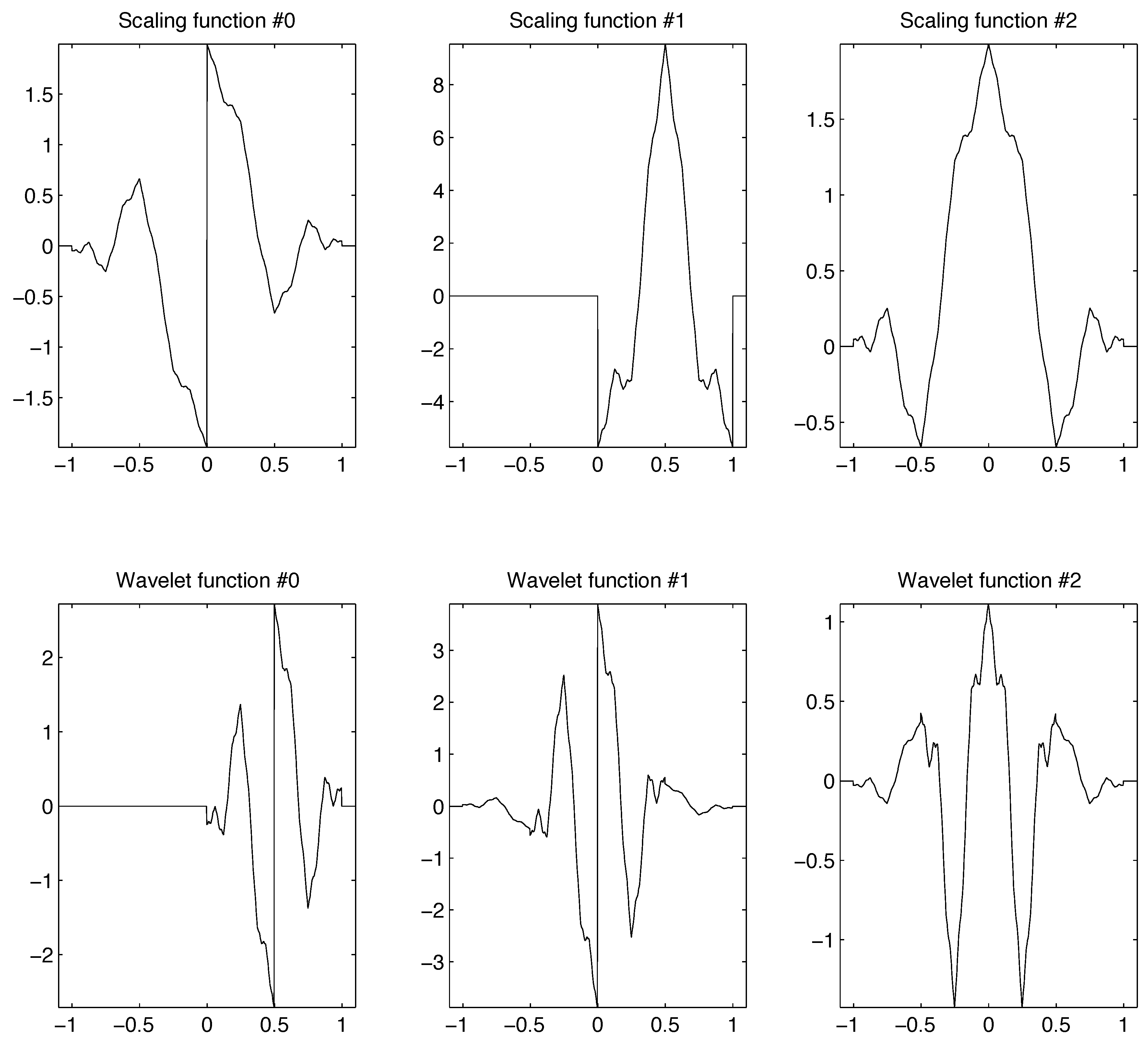
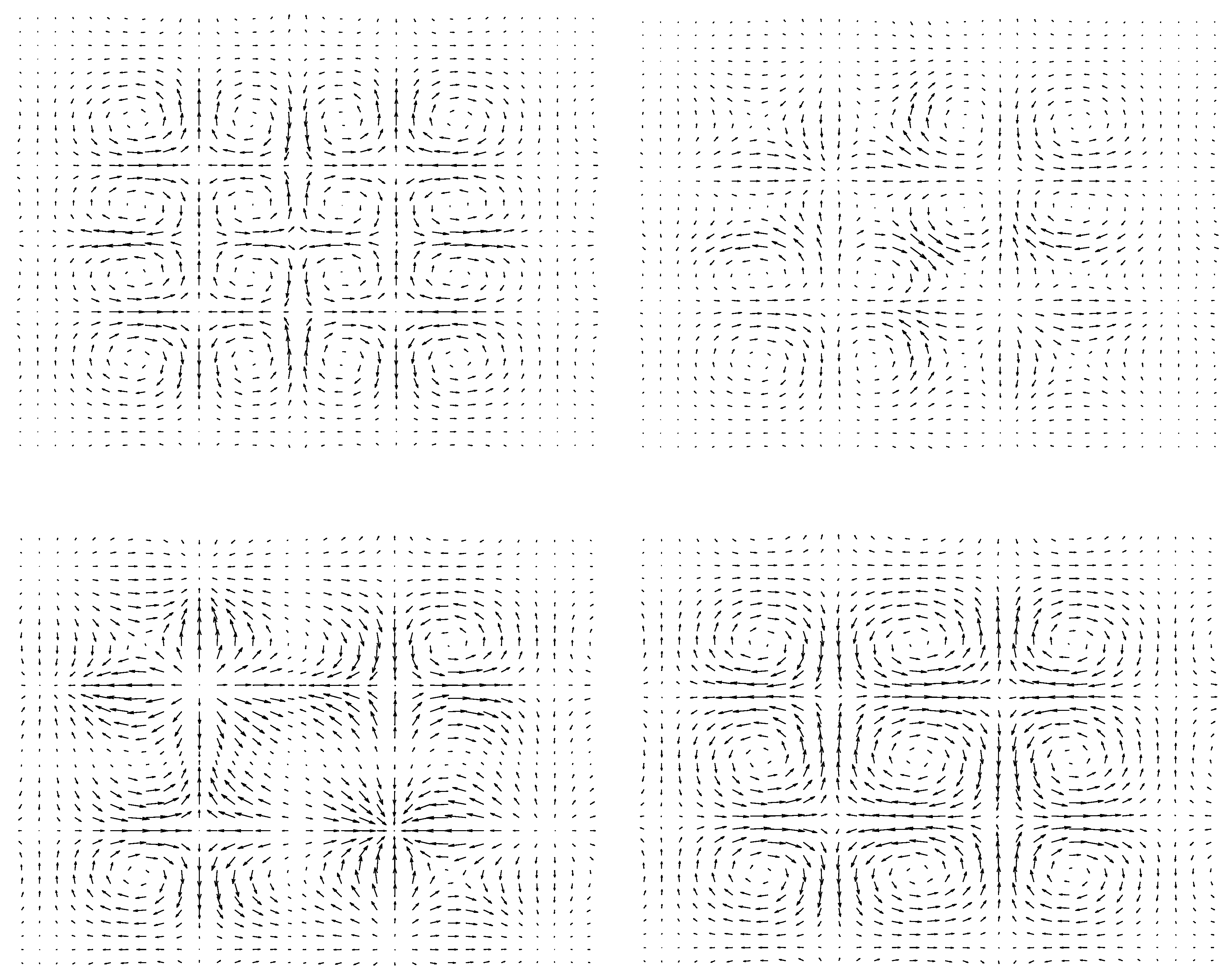
Each one of the divergence-free multiwavelets ${\overrightarrow{\tilde{\Psi }}}_{\partial ,\ell },{\overrightarrow{\tilde{\Psi }}}_{\text{int},\ell },\ell =1,2,3,$ consists of nine components. Figure 4 plots some of the components of ${\overrightarrow{\tilde{\Psi }}}_{\text{int},1}$.

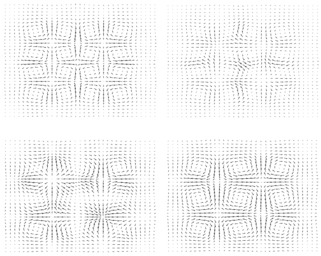
Figure 4. Some components of ${\overrightarrow{\tilde{\Psi }}}_{\text{int},1}$.

Figure 4. Some components of ${\overrightarrow{\tilde{\Psi }}}_{\text{int},1}$.

4. Conclusions

We have constructed vector wavelet families on the upper half plane ${\mathbb{R}}_{+}^2$ such that the reconstructing wavelets are divergence-free and piecewise $C^1$ and form a basis for the closed subspace $H^0(\mathrm{div},{\mathbb{R}}_{+}^2)$. In contrast to previous constructions, the boundary components satisfy a vanishing normal boundary condition desirable for applications. The boundary constraints and desire for short supports suggest the use of wavelets built on fractal interpolation functions. To build in the divergence-free property we use certain commutation conditions made possible through Strela’s two-scale transform. Because these wavelets are built via tensor products, analogues can be built in dimensions of three and higher.

References

- Battle, G.; Federbush, P. Divergence–free vector wavelets. Michigan Math. J. 1993, 40, 181–195. [Google Scholar] [CrossRef]
- Lemarié-Rieusset, P.G. Un théorème d’inexistence pour les ondelettes vecteurs à divergence nulle. C. R. Acad. Sci. Paris Se´r. I Math. 1994, 319, 811–813. [Google Scholar]
- Lemarié-Rieusset, P.G. Analyses multi-résolutions non orthogonales, commutation entre projecteurs et dérivation et ondelettes vecteurs à divergence nulle. Rev. Mat. Iberoamericana 1992, 8, 221–237. [Google Scholar] [CrossRef]
- Urban, K. On divergence–free wavelets. Adv. Comput. Math. 1995, 4, 51–81. [Google Scholar] [CrossRef]
- Urban, K. Wavelet bases in H(div) and H(curl). Math. Comput. 2001, 70, 739–766. [Google Scholar] [CrossRef]
- Urban, K. Wavelets in Numerical Simulation; Springer–Verlag: Berlin, Germany, 2002. [Google Scholar]
- Albukrek, C.; Urban, K.; Rempfer, D.; Lumley, J. Divergence–free wavelet analysis of turbulent flows. J. Sci. Comput. 2002, 17, 49–66. [Google Scholar] [CrossRef]
- Kelliher, J. Navier–Stokes equations with Navier boundary conditions for a bounded domain in the plane. SIAM J. Math. Anal. 2006, 38, 210–232. [Google Scholar] [CrossRef]
- Nguyen, P. Biorthogonal multiwavelets adapted to boundary value problems. Ph.D. Thesis, New Mexico State University, Las Cruces, NM, USA, 2012. [Google Scholar]
- Strela, V. Multiwavelets: Theory and applications. Ph.D. Thesis, Massachusetts Institute of Technology, Boston, MA, USA, 1996. [Google Scholar]
- Donovan, G.; Geronimo, J.; Hardin, D. Fractal functions, splines, intertwining multiresolution analysis and wavelets. Proc. SPIE 1994, 2303, 238–243. [Google Scholar]
- Massopust, P. A multiwavelet based on piecewise C1 fractal functions and related applications to differential equations. Bol. Soc. Mat. Mexicana 1998, 4, 249–283. [Google Scholar]
- Lakey, J.; Pereyra, M.C. Divergence–free Multiwavelets on Rectangular Domains. In Wavelet Analysis and Multiresolution Methods (Lecture Notes in Pure and Applied Mathematics); He, T.-X., Ed.; Dekker: New York, NY, USA, 2000; pp. 203–240. [Google Scholar]
© 2013 by the authors; licensee MDPI, Basel, Switzerland. This article is an open access article distributed under the terms and conditions of the Creative Commons Attribution license (http://creativecommons.org/licenses/by/3.0/).