Statistical Invariants for Classification on Tiny Datasets

Abstract

We investigate the influence of statistical invariants for classification problems on tiny datasets. We present a review of current state-of-the-art methods for classification, with a brief discussion of the differences and trade-offs between the proposed method and existing classifiers. Then, we lay out the philosophical and mathematical foundations of the statistical theory of learning, incorporating the discovery of statistical invariants. We derive algorithmic implementations for binary, multiclass, and multilabel classification alongside technical details and recommendations for practitioners. We demonstrate the efficacy of the proposed algorithm through comparative studies against state-of-the-art AutoML frameworks on a benchmark suite.

1. Introduction

The mathematical theory of learning constructs inductive methods that converge to the desired function (underlying generative process) with an increasing number of observations. Learning theory must provide the practitioner with the following guarantees [1]:

• Necessary and sufficient conditions for consistency (predictions converge to the desired function).
• Necessary and sufficient conditions for generalization (error bounds).

Unfortunately, for most problems, these requirements are not sufficient. Practitioners have limited resources and limited access to datasets that are usually small.

The trend toward larger datasets is apparent rather than real. One dataset dominates the tail: the internet. Dataset size (the number of samples, not the dimension) follows a Pareto distribution, so most predictions rest on small and tiny data [2,3]. In fact, most datasets fit on a single commercial laptop; this is what we call small data.

Embedded systems and the Internet of Things (IoT) [4] impose even sharper storage and compute constraints, and thus operate on tiny data. This setting has produced a subfield called TinyML, which develops models for such constrained systems [5,6]. We recast the learning problem as one of finding the desired dependence using a limited number of observations [7]. We also need to construct algorithms with proof of correctness, fast rates of convergence, and numerical stability.

Automated machine learning (AutoML) dominates business practice in the medium, small, and tiny data space because it achieves high scores efficiently, costs relatively little, and remains easy to implement for experts and non-experts [8]. AutoML frameworks use ensemble methods that train large families of distinct models and return the best prediction or a weighted average of the predictions. Ensemble methods introduce ideas such as stacking, bagging, and boosting. In these methods, each isolated (weak) learner attempts to learn the function and is then combined into a strong learner. Bagging (bootstrap aggregation) trains models in parallel on subsets of the dataset and, once combined, approximates the Bayes posterior [9], which reduces the variance. Theorems establish the consistency and exponential generalization properties of bagging [10].

Boosting samples sequentially, weighting the examples that previous models misclassified in order to reduce the bias [11]. Boosting has theoretical underpinnings in the Weak Learner theorem [12] and some generalization theorems. Ensemble methods are especially susceptible to picking up noise [13] and overfitting. Reusing the same shuffle across models causes overfitting, so ensemble methods demand careful training [14]. These methods attempt to reach the highest score at any cost and often engage in subtle forms of data-snooping, which the given error estimates usually omit [15]. Many winning solutions in competitions [16,17] use ensemble methods, including boosting algorithms such as XGBoost or LightGBM [18,19], although most of these techniques lack proof of either consistency or generalization.

In this space, the framework AutoGluon frees the user from algorithm selection and hyperparameter tuning [20]. The 4-h extreme version is currently the ceiling of the state of the art on TabArena [21], a benchmark for machine learning on tabular data. This framework remains competitive on Kaggle [20], a platform biased toward rewarding the highest scorer.

The lack of solid theoretical foundations for such models presents a challenge to researchers, either to encourage them to fill in these theoretical gaps or to find simpler solutions to the learning problem. This work derives, in mathematically rigorous form, a recent idea in learning theory: statistical invariants. Furthermore, we provide algorithms for binary, multiclass, and multilabel classification with practical recommendations for their respective numerical implementations. This theory offers an alternative, simpler solution that fills the research gap.

2. Statistical Learning Using Invariants

The main problem of pattern recognition (classification) can be stated as follows: a learning machine observes a finite training set $\{(x_1,y_1),\dots ,(x_n,y_n)\}$ drawn i.i.d. from a joint distribution $p_{X,Y}(x,y)=p_{Y|X}\left(y\right|x)p_X\left(x\right)$, where a classifier reacts to events $x_i\in {\mathbb{R}}^d$ with a binary signal $y_i\in \{0,1\}$ using a fixed but unknown distribution $p_{Y|X}(y=1|x_i)$, while $p_X\left(x\right)$ is some underlying inaccessible generative process.

The problem is to find, in a given set of functions, the one that minimizes the probability of error between classifications. In other words, to train or fit a model that outputs $\widehat{y}$ given new unseen inputs x so that the probability of incorrect classifications ($y\ne \widehat{y}$) is minimized. A solution to this problem is as follows: instead of finding indicator functions, we estimate the conditional probability directly using the data [22].

Let $f\left(x\right)=\mathbb{P}(y=1|X=x)$ be the desired function. By the definition of the joint probability:

$$p_{X,Y}(x,y=1)=p_X\left(x\right)p_{Y|X}(y=1|x)=p_X\left(x\right)f\left(x\right).$$

Then consider a generalization of its CDF:

$$F(x,y=1)=\mathbb{P}(X\le x,Y=1)=\int \mathbf{1}[\xi \le x]p_X\left(\xi \right)f\left(\xi \right)d\xi .$$

(1)

The weak derivative D of the step function $\mathbf{1}[·]$ is the Dirac delta. Differentiating the CDF under the integral sign, we have:

$$D_{x}F(x,y=1)=p_{X,Y}(x,y=1)=\int D_x\mathbf{1}[\xi \le x]p_X\left(\xi \right)f\left(\xi \right)d\xi$$

$$=\int \delta (\xi -x)p_X\left(\xi \right)f\left(\xi \right)d\xi =p_X\left(x\right)f\left(x\right).$$

Now replace the left-hand side of Equation (1) by its empirical estimate (Glivenko–Cantelli theorem [7]) and the expected value on the right-hand side by its sample average:

$${\displaystyle \frac{1}{n}}{\displaystyle \sum _{j=1}^n}\mathbf{1}[x_j\le x]y_j\approx {\displaystyle \frac{1}{n}}{\displaystyle \sum _{i=1}^n}\mathbf{1}[x_i\le x]f\left(x_i\right),$$

(2)

where we cannot use a strict equality because we use a finite sample.

Thus, Equation (2) is a family of equations depending on the notion of equality. To solve one of them means finding the function minimizing a chosen error measure. We choose the squared error to get a convex problem:

$$R\left[f\right]=\int {\left({\displaystyle \frac{1}{n}}{\displaystyle \sum _{j=1}^n}\mathbf{1}[x_j\le x]y_j-{\displaystyle \frac{1}{n}}{\displaystyle \sum _{i=1}^n}\mathbf{1}[x_i\le x]f\left(x_i\right)\right)}^{2}dF\left(x\right)$$

$$={\displaystyle \sum _{i,j=1}^n}(f\left(x_i\right)-y_i)(f\left(x_j\right)-y_j)V_{ij},$$

where

$$V_{ij}=\int \mathbf{1}[x_i\le x]\mathbf{1}[x_j\le x]dF\left(x\right)\approx {\displaystyle \frac{1}{n}}{\displaystyle \sum _{k=1}^n}\mathbf{1}[x_i\le x_k]\mathbf{1}[x_j\le x_k].$$

The matrix V is a Gram matrix and therefore positive semi-definite of size $n\times n$.

Unfortunately, Equation (1) is ill-posed; this means that it is not enough to minimize the empirical risk. To solve the empirical estimate in Equation (2) correctly, we use the theory of regularization [23]. We accomplish this by introducing a functional g that controls the diversity (capacity) of the set of functions. For practical applications, we need to choose properties that align with the intended optimization approach [24]; therefore, we require g to be at least positive, continuous, and convex.

The regularized empirical risk is therefore:

$$R\left[f\right]=(1-\rho ){(f-y)}^{\mathsf{T}}V(f-y)+\rho g\left(f\right),$$

(3)

where $\rho$ is the regularization strength. The desired function must minimize this regularized risk functional on the training dataset. If the VC dimension of the set of functions is finite, then this procedure is consistent [25]; furthermore, we can provide error bounds. Let the VC dimension of our set of functions be h. Then, for a training set of size n, with probability $1-\delta$ the expected prediction error on unseen data $R\left[f\right]$ is bounded by the empirical error $\widehat{R}\left[f\right]$ and a term depending on n, h, and $\delta$ [24]:

$$R\left[f\right]\le \widehat{R}\left[f\right]+{\displaystyle \frac{\eta }{2}}\sqrt{1+{\displaystyle \frac{4\widehat{R}\left[f\right]}{\eta }}},$$

(4)

where

$$\eta ={\displaystyle \frac{c_1}{n}}\left(h\left(1+ln(c_{2}n/h)\right)-ln\left(\delta /4\right)\right)$$

and

$$0<c_1\le 4,0<c_2\le 2.$$

In practice, a tighter bound requires union bounds over the model-selection procedure and empirical estimates of $c_1$ and $c_2$.

2.1. Predicates and Statistical Invariants

The philosophical theory of statistical invariants stems from the Platonist worldview; that there are concepts in the world of ideas (predicates) that are instantiated and realized in the world of things and fed to the learning process (invariants). Each domain carries its own concepts: images contain edges and parallel lines, together with rotational, translational, and mirror symmetry. The theory rests on the idea that learners must embody knowledge independent of the data.

The mathematical justification of these invariants is based on the notions of convergence in a Hilbert space; we say that a sequence of functions $f_n$ converges to f strongly if the $L_2$ distances tend to 0 as n grows beyond all bounds. Similarly, we say that a sequence $f_n$ converges weakly to f if for all test functions $\varphi \in L_2$,

$$\underset{n\to \infty }{lim}\langle f_n-f,\varphi \rangle =0.$$

In our case, the sequence of estimates converges to $f\left(x\right)=\mathbb{P}(y=1|x)$ weakly if for all $\varphi \in L_2$:

$$\underset{n\to \infty }{lim}\int \varphi \left(x\right)f_n\left(x\right)p_X\left(x\right)dx=\int \varphi \left(x\right)p_{Y,X}(y=1,x)dx.$$

(5)

The strong mode of convergence implies the weak mode; the converse is true only if the set of functions is compact [26]. Consider now a finite set of test functions, called predicates ${\varphi }_s\left(x\right):{\mathbb{R}}^d\to {\mathbb{R}}^{r_s}$, $r_s\in \mathbb{N}$ and $s=1,\dots ,m$. Replacing the probability densities in Equation (5) with their empirical estimates and all test functions with the finite set of predicates, we have:

$${\displaystyle \frac{1}{n}}{\displaystyle \sum _{i=1}^n}{\varphi }_s\left(x_i\right)f\left(x_i\right)={\displaystyle \frac{1}{n}}{\displaystyle \sum _{i=1}^n}{\varphi }_s\left(x_i\right)y_i\mathrm{for}s=1,\dots ,m.$$

(6)

These equalities are the statistical invariants associated with the predicates, then:

$${\Phi }_s^{\mathsf{T}}f={\Phi }_s^{\mathsf{T}}y\mathrm{for}s=1,\dots ,m.$$

This leads to $r=\sum r_s$ equalities, although in practice each $r_s$ is usually either 1, d, or n, which are the intrinsic dimensions of the problem. The predicate matrix can be normalized (for example, $\parallel \Phi \parallel =1$), depending on the numerical implementations of the solvers.

When the dataset is tiny, these equalities are overly strict; we obtain a more general formulation using the Hoeffding inequality [25], for bounded functions of random variables $a\le u\left(x\right)\le b$ and any $\epsilon >0$:

$$\mathbb{P}\left(\left|\int u\left(x\right)dF\left(x\right)-{\displaystyle \frac{1}{n}}{\displaystyle \sum _{i=1}^n}u\left(x_i\right)\right|\ge \epsilon \right)\le 2exp\left(-{\displaystyle \frac{2n{\epsilon }^2}{{(b-a)}^2}}\right).$$

Therefore, with probability $1-\delta$ the following holds:

$$\left|{\displaystyle \sum _{i=1}^n}{\varphi }_s\left(x_i\right)y_i-{\displaystyle \sum _{j=1}^n}{\varphi }_s\left(x_j\right)f\left(x_j\right)\right|⪯(b_s-a_s)\sqrt{{\displaystyle \frac{nln(2/\delta )}{2}}},$$

(7)

for $s=1,\dots ,m$, where $a_s=\min {\varphi }_s\left(x_i\right)$ and $b_s=\max {\varphi }_s\left(x_i\right)$, and inequalities are component-wise.

2.2. Examples of General Predicates and Invariants

• ${\Phi }^{\mathsf{T}}\left(X\right)=1_n^{\mathsf{T}}\in {\mathbb{R}}^{1\times n}$: forces f to respect the frequency of the examples in the class $y=1$ as seen in the training data.
• ${\Phi }^{\mathsf{T}}\left(X\right)=X^{\mathsf{T}}\in {\mathbb{R}}^{d\times n}$: forces the center of mass of f to be the same as the center of mass of the class $y=1$ with respect to the training data.
• ${\Phi }^{\mathsf{T}}\left(X\right)=X{X}^{\mathsf{T}}\in {\mathbb{R}}^{n\times n}$: forces the empirical second moment of f to match that of the class $y=1$.

2.3. Examples of Domain-Specific Invariants

• Images: Vertical and horizontal symmetry, tangent-distance operators, Lie derivatives [25].
• Medical (diabetes problem): From previous experience, a medical doctor knows that a closed and connected region B in the BMI vs. Glucose subspace is representative of patients with diabetes in the local area. The doctor proposes the following predicate $\varphi \left(x_i\right)=\mathbf{1}[x_i\in B]$ [25].

We contrast the formal concept of invariants with feature engineering. On one hand, with an increasing number of features, the capacity of our hypothesis space (VC dimension) increases, which necessitates an increase in the size of training data. On the other hand, with an increasing number of invariants, the capacity of our hypothesis space decreases. In the limit, as we increase the number of correctly formulated invariants, the hypothesis space shrinks to a set with a single function: the desired one [25].

2.4. Solution of the Learning Problem

We estimate the conditional probability $\mathbb{P}(y=1|x)$ in a Reproducing Kernel Hilbert Space (RKHS) of functions of bounded norm, which is weakly compact [26]. Let the desired function have the following form (by the representer theorem [27]):

$$\mathbb{P}(y=1|x)=f\left(x\right)={\displaystyle \sum _{i=1}^n}{\alpha }_{i}K(x,x_i)=\langle \alpha ,k\left(x\right)\rangle ,$$

where $k\left(x\right)={(K(x,x_1),\dots ,K(x,x_n))}^{\mathsf{T}}\mathrm{size}n\times 1$; this is the kernel basis expansion of the data, as an example consider the Gaussian kernel:

$$K(x,x_0)=exp\left(-\gamma \parallel x-x_0{\parallel }^2\right),$$

where $\gamma$ is a free parameter that controls the width of the kernel.

Let the capacity of the hypothesis space be:

$$g\left(f\right)={\parallel f(x,\alpha )\parallel }_2^2={\displaystyle \sum _{i,j=1}^n}{\alpha }_i{\alpha }_{j}K(x_i,x_j)=\langle \alpha ,K\alpha \rangle ,$$

where in this context $K=K(x_i,x_j)$ is a positive semi-definite kernel matrix of size $n\times n$. Then, we select m predicates which capture aspects of the particular generative process and mathematical structure of the domain:

$${\varphi }_s\left(x\right):{\mathbb{R}}^d\to {\mathbb{R}}^{r_s},r_s\in \mathbb{N},s=1,\dots ,m{\displaystyle \sum _{s=1}^m}{r}_s=r.$$

The desired function minimizes the regularized risk functional of Equation (3):

$$R\left[\alpha \right]=(1-\rho )(\langle K\alpha ,VK\alpha \rangle -2\langle K\alpha ,Vy\rangle )+\rho \langle \alpha ,K\alpha \rangle$$

(8)

subject to $2r$ inequality constraints based on the invariants in Equation (7), plus $2n$ inequalities (n on each side):

$$0_n⪯K\alpha ⪯1_n$$

(9)

expressing that the conditional probability is non-negative and bounded by 1. These equations have the form of a general quadratic program (QP):

$$\begin{array}{c}\hfill \underset{\alpha \in {\mathbb{R}}^n}{\min }{\displaystyle \frac{1}{2}}{\alpha }^{\mathsf{T}}P\alpha +q^{\mathsf{T}}\alpha \\ \hfill \mathrm{s}.\mathrm{t}.G\alpha ⪯h,\end{array}$$

where the inequality constraints are component-wise. If P is positive semi-definite, then the QP is convex [28], and the solver converges to the global minimum with numerical stability. Even though the theoretical worst-case complexity of QP is high, in practice it converges in fewer than a hundred iterations [29,30]. In a QP, $\alpha$ denotes the desired vector ($\alpha =({\alpha }_1,\dots ,{\alpha }_n)$), the weights of the kernel basis expansions on the training data. After some manipulations of Equations (7)–(9), the matrices P and G and the vectors q and h are:

$$P=2\left((1-\rho )K^{\mathsf{T}}VK+\rho K\right)(n\times n),$$

$$q^{\mathsf{T}}=-2(1-\rho )y^{\mathsf{T}}VK(1\times n).$$

Let

$$\Phi =\left(\begin{array}{c}{\Phi }_1^{\mathsf{T}}\left(X\right)\\ {\Phi }_2^{\mathsf{T}}\left(X\right)\\ ⋮\\ {\Phi }_m^{\mathsf{T}}\left(X\right)\end{array}\right)(r\times n),\epsilon =\sqrt{nln(2/\delta )/2}\left(\begin{array}{c}{b}_1-a_1\\ b_2-a_2\\ ⋮\\ b_r-a_r\end{array}\right)(r\times 1),$$

then:

$$G=\left(\begin{array}{c}\Phi K\\ -\Phi K\\ K\\ -K\end{array}\right)(2(r+n)\times n),h=\left(\begin{array}{c}\epsilon +\Phi y\\ \epsilon -\Phi y\\ 1_n\\ 0_n\end{array}\right)(2(r+n)\times 1).$$

Here, P is positive semi-definite because it is a convex combination of positive semi-definite matrices. This leads naturally to the training algorithm. We call this model LUSI (learning using statistical invariants) and write LUSI+ for the model that adds the predicate constraints.

2.4.1. Algorithm: Fit LUSI

Algorithm 1 lists the fitting procedure.

Algorithm 1 Fit LUSI

Input: Training data $X=(x_1,\dots ,x_n)\in {\mathbb{R}}^{n\times d}$  Input: Labels $y=(y_1,\dots ,y_n)\in {\{0,1\}}^n$  Input: m predicates ${\Phi }_s:{\mathbb{R}}^d\to {\mathbb{R}}^{r_s},r_s\in \mathbb{N},s=1,\dots ,m$  Input: Regularization constant $\rho \in [0,1]$  Input: PSD kernel $K:{\mathbb{R}}^d\times {\mathbb{R}}^d\to \mathbb{R}$  Input: Error level $\delta \in (0,1)$ (e.g., 0.05)  Form matrices P, q, G, h defined above  Feed to a QP solver and get $\alpha$  Output: $\alpha$

The error level $\delta$ is chosen proportional to the smallness of the dataset.

The computational complexity of this algorithm depends on the implementation of the QP solver and is roughly $O\left(n^3\right)$, although interior point methods converge quickly in practice, often in the order of tens of iterations [30].

The set of predicates $\Phi$ must be consistent; if the tolerances are too strict or the predicates contradict each other, then the feasible region becomes empty. A possible strategy adds predicates incrementally.

Finally, even though P is theoretically positive semi-definite, in practice it may be ill-conditioned; therefore, a correct implementation of this algorithm must handle this case gracefully.

2.4.2. Algorithm: Predict LUSI

After training, the coefficients $\alpha$ give the kernel basis expansion of the conditional probability, which Algorithm 2 evaluates at a new datapoint.

Algorithm 2 Predict LUSI

Input: New datapoints x  Compute $f\left(x\right)=\langle k\left(x\right),\alpha \rangle$  Output: $f\left(x\right)=\mathbb{P}(y=1|x)$

The model outputs the probability that the datapoint x belongs to the class $y=1$. Depending on the implementation of the preprocessing scalers, inputs x outside the training dataset can yield $f\left(x\right)<0$ or $f\left(x\right)>1$; therefore, a correct implementation of this algorithm must clip such values.

2.5. Classification Methods

2.5.1. Binary Classification

With the model prediction in hand, we can perform binary, multiclass, and multilabel classification by introducing a threshold $p_0$ for the probability, depending on the application, but typically set to 0.5. Algorithm 3 applies this threshold.

Algorithm 3 Binary classification LUSI

Input: New datapoint x  Compute $f\left(x\right)=\mathbb{P}(y=1|x)$ using Predict LUSI.  Assign $\widehat{y}=\mathbf{1}[f\left(x\right)\ge p_0]$.  Output: $\widehat{y}$

2.5.2. Multiclass Classification

Let $Y=\{1,2,\dots ,k\}$ be a set of k mutually exclusive classes. The binary classifier admits two extensions: one-vs-rest (OVR) or one-vs-one (OVO).

• OVR: Trains k classifiers, one for each class against the rest, which is prohibitive on large n. Complexity $O\left(k{n}^3\right)$.
• OVO: Trains $k(k-1)/2$ classifiers, pitting each class against each other. If the dataset is balanced, then each classifier trains on $2n/k$ datapoints, with complexity $O(n^3/k)$.

Depending on the dataset size and the number and balance of the classes, choose the strategy with lower complexity. OVO becomes more interpretable when pairwise comparison of labels matters.

Let $f_i\left(x\right)=\mathbb{P}(y=i|x)$ be the probability given by the ith classifier against the rest. We select the most likely class, as Algorithm 4 shows.

Algorithm 4 OVR Multiclass Classification LUSI

Train k classifiers.  Assign $\widehat{y}=argmax\{f_1\left(x\right),\dots ,f_k\left(x\right)\}$  Output: $\widehat{y}$

For OVO classification, let $p_{ij}$ be the probability of class i over j ($i,j\in \{1,\dots ,k\}$ and $i\ne j$), obtained by training a classifier on a subset of the training data containing only labels $i,j$. Observe that $p_{ji}=1-p_{ij}$. In total, we train $k(k-1)/2$ classifiers. We select the class that wins most often against the others. Let ${\widehat{y}}_i={\sum }_{j\ne i}{p}_{ij}$. Select the class with the highest sum, as Algorithm 5 shows.

Algorithm 5 OVO Multiclass Classification LUSI

Train $k(k-1)/2$ classifiers.  Compute ${\widehat{y}}_i={\sum }_{j\ne i}{p}_{ij}$ for each class i.  Assign $\widehat{y}=argmax\{{\widehat{y}}_1,\dots ,{\widehat{y}}_k\}$  Output: $\widehat{y}$

The probability of a class follows from normalizing the sum of the pairwise probabilities over all other classes.

2.5.3. Multilabel Classification

Instead of selecting a single label based on the maximum probability, for a new prediction we select all labels with a probability of at least $p_0$. Algorithm 6 applies this rule to every label.

Algorithm 6 OVR Multilabel classification LUSI

Train k classifiers.  Assign $\widehat{y}=argwhere\{\mathbf{1}[f_1\left(x\right)\ge p_0],\dots ,\mathbf{1}[f_k\left(x\right)\ge p_0]\}$  Output: $\widehat{y}$

The operator $argwhere\{·\}$ returns the indices of the elements in the array that equal 1 (or that evaluate to true). OVO cannot produce consistent multilabel assignments.

We present a simple example to illustrate the clarity and interpretability of these algorithms. Suppose we have a multilabel dataset such as Mediamill, which consists of video keyframes and associated semantic labels such as ‘crowd’, ‘sports’, and ‘indoor’, which represent overlapping concepts. A video carries several concepts at once. For simplicity, assume we are working with only these three labels. Our goal is to identify the relevant concepts for a new video.

We train three LUSI models in an OVR fashion using Algorithm 1, with predicates ${\Phi }_1$ and ${\Phi }_2$ as defined in Section 2.2, an error level $\delta =0.05$, a Gaussian kernel, and regularization constant $\rho =0.1$. We construct P, q, G, and h and provide them to a QP solver. This program finds $f\left(x\right)$, the unique optimal solution that minimizes the regularized risk functional in Equation (8). The solver reaches this solution efficiently and with numerical stability.

Given a new datapoint x, for each label i we compute $f_i\left(x\right)$, the probability that x belongs to class i, using Algorithm 2 for each of the three models. Suppose we obtain $f=\{f_1\left(x\right),f_2\left(x\right),f_3\left(x\right)\}=\{0.6,0.4,0.93\}$.

These probabilities express the confidence that LUSI assigns to each label. This information helps decision makers by providing a measure of certainty in the assignments. For example, 0.6 and 0.4 sit close to 0.5 and leave the decision about a crowd or a sports event unresolved. However, the probability for the ‘indoor’ label is high, increasing the decision maker’s confidence.

If we assign multiple labels regardless, then we set the decision threshold $p_0=0.5$ and use Algorithm 6 to assign the labels. Therefore,

$$\widehat{y}=argwhere\{\mathbf{1}[0.6\ge 0.5],\mathbf{1}[0.4\ge 0.5],\mathbf{1}[0.93\ge 0.5]\}=\{1,3\}.$$

We thus label x as ‘crowd’ and ‘indoor’.

2.6. Advantages of the LUSI Family of Models for Classification

• Philosophical and mathematical underpinnings, with theorems on consistency and error bounds.
• A proof of convergence to the global minimum.
• Interpretable probabilities for decision makers.

Open questions in the statistical theory of learning include the discovery of useful kernels, the choice of predicates, efficient model selection, and the computational challenges of the deduced algorithms on particular datasets.

3. Materials and Methods

We studied LUSI and LUSI+ empirically. We compared their performance to state-of-the-art classifiers using a benchmark suite. The suite consisted of the 164 curated classification datasets of the Penn Machine Learning Benchmark (PMLB) version 1.0.1 [31].

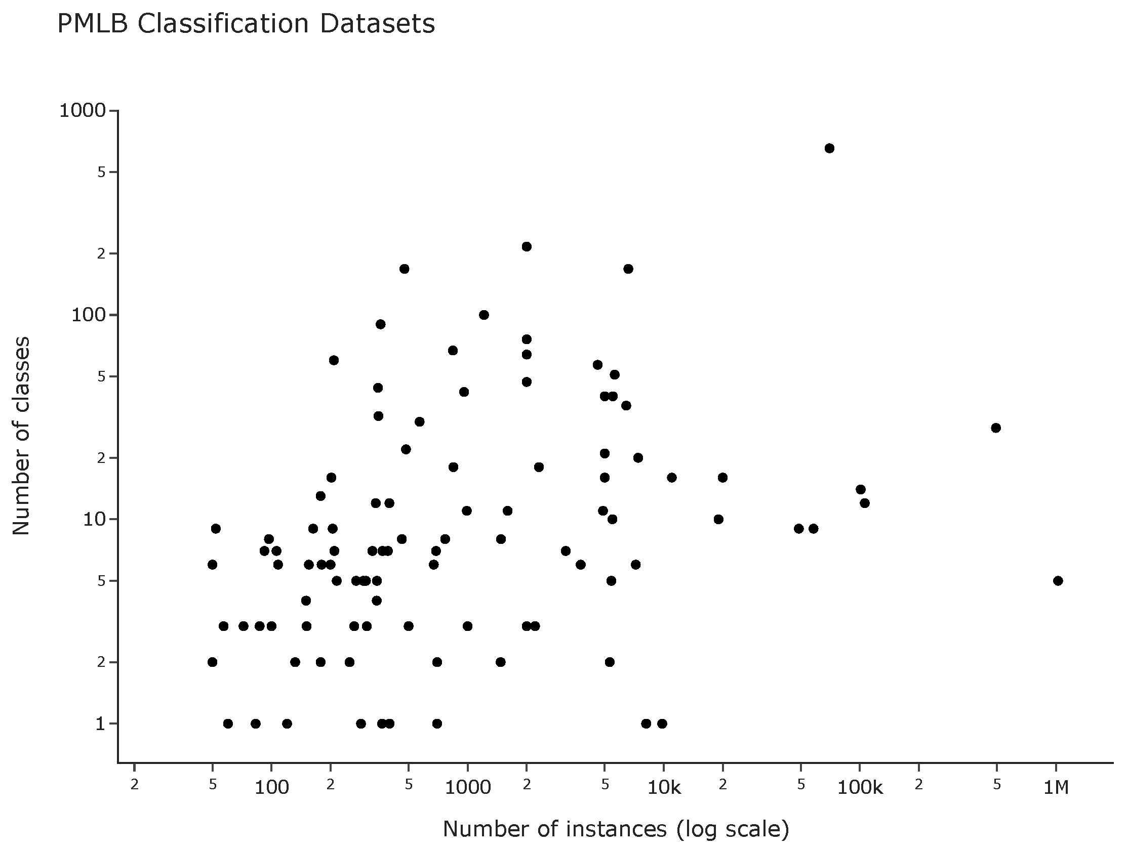
The dataset distribution in Figure 1 shows clustering near smaller sample sizes (<10 k instances) and fewer than five classes, consistent with our claim that most datasets are small or tiny.

We conducted a benchmark comparison on the smallest 100 (by number of instances) datasets of the original suite, called run $\times 1$, and three reduced versions thereof: $\times 2$, $\times 5$, and $\times 10$ smaller datasets for a total of four experiments called runs. The last run strains the classifiers’ generalization ability, because the number of instances is tiny.

We compared four model classes: a baseline linear SVC, AutoGluon, LUSI, and LUSI+. LUSI and LUSI+ used Gaussian kernels, without and with predicates respectively. The dataset domains are diverse (social, biological/medical, agricultural sciences, physics, images, games, dynamical systems, and artificial datasets), making domain-specific invariants impractical for reproducibility in this study. Therefore, we restricted the study to a set of general mathematical predicates (predicates 1 and 2 in Section 2.2), applied equally to all datasets.

One of the main hypotheses of this study is that introducing invariants improves the score of the models by capturing additional regularity or extracting more information related to the underlying generative process.

We used AutoGluon v.1.2 with the package defaults, which use their own preprocessing and validation pipelines. We allocated a fitting budget of $n/1000$ h and used the system defaults for reproducibility, because AutoGluon runs longer without a cap. The hardware consisted of a MacBook Pro 16-inch 2021 M1 Pro with 16 GB of RAM, running macOS Sequoia 15.5.

The proposed models LUSI and LUSI+ require simple data preprocessing because these models use metric-based scalers [32]. We remained neutral about outliers or features with missing values and abstained from dropping columns or instances; we one-hot encoded categorical features and grouped rare values into a new category. These datasets contain no missing categorical values. For simplicity, we used $V=I_n$ as the identity matrix in the experiments.

We imputed the missing values of continuous features with the median and scaled them with the scikit-learn robust scaler [33], which avoids dropping or clipping outliers. The model selection strategy used a $10\times 10$ grid search in log-space ($-3$ to 6 in steps of 1) for the kernel parameter and 10 values of the regularization parameter (from 0 to 1 in steps of 0.1) with cross-validated balanced accuracy in the inner loop as the score function.

The SVC model received the same preprocessing as LUSI and LUSI+.

4. Results

Score per Run: $\times 1$, $\times 2$, $\times 5$, $\times 10$

Scores on each dataset were computed as the mean balanced accuracy over repeated splits. The $\times 1$ run used cross-validation; for the reduced versions, each fold is an independent train/test split at the stated holdout ratio. The reduced versions retain the class imbalance of the original dataset, with a minimum class count of one. Every model received the same version.

For the $\times 1$ run, we computed the mean scores of a 3-fold cross-validation with a 20% holdout set. For the $\times 2$ run, we computed the mean scores of a 3-fold cross-validation with a 50% holdout set. For the $\times 5$ run, we computed the mean scores of a 5-fold cross-validation with a 75% holdout set. For the $\times 10$ run, we computed the mean scores of a 10-fold cross-validation with a 90% holdout set.

The following metrics were computed on each dataset: balanced accuracy, F1 score, sensitivity, and runtime. These are summarized in

Table 1. Median scores for run ×1. Best value in each column in bold.

Model	Balanced Acc.	F1	Sensitivity	Runtime (s)
AutoGluon	0.823	0.827	0.841	179.2
LUSI+	0.817	0.817	0.833	4.40
LUSI	0.812	0.816	0.833	3.30
SVC	0.746	0.748	0.804	0.001

,

Table 2. Median scores for run ×2. Best value in each column in bold.

Model	Balanced Acc.	F1	Sensitivity	Runtime (s)
AutoGluon	0.796	0.791	0.811	89.0
LUSI+	0.775	0.779	0.809	1.80
LUSI	0.771	0.778	0.816	1.32
SVC	0.734	0.735	0.784	0.001

,

Table 3. Median scores for run ×5. Best value in each column in bold.

Model	Balanced Acc.	F1	Sensitivity	Runtime (s)
LUSI+	0.754	0.763	0.800	1.06
LUSI	0.754	0.757	0.812	0.650
AutoGluon	0.748	0.754	0.798	54.5
SVC	0.710	0.710	0.769	0.001

and

Table 4. Median scores for run ×10. Best value in each column in bold.

Model	Balanced Acc.	F1	Sensitivity	Runtime (s)
LUSI	0.671	0.673	0.756	0.270
SVC	0.659	0.651	0.729	0.001
LUSI+	0.626	0.623	0.735	0.700
AutoGluon	0.558	0.543	0.696	6.67

.

As an example, for the $\times 5$ run, we used 5 folds; on each fold we trained the model with 25% of the data and tested on the remaining 75%. We averaged the scores over the folds, repeated the process for each dataset, and reported the median in the table.

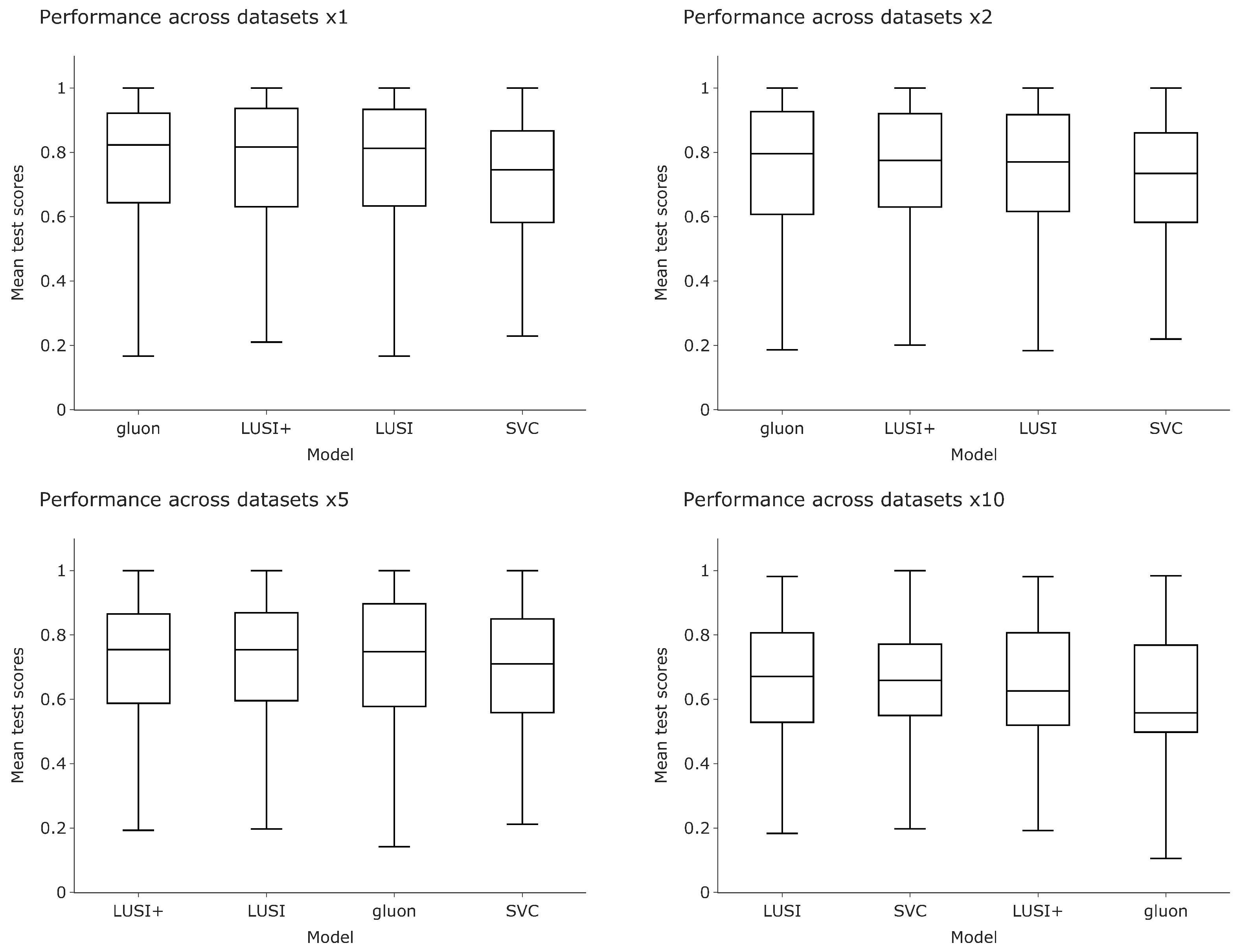
We present the distribution of balanced accuracy in a boxplot in Figure 2.

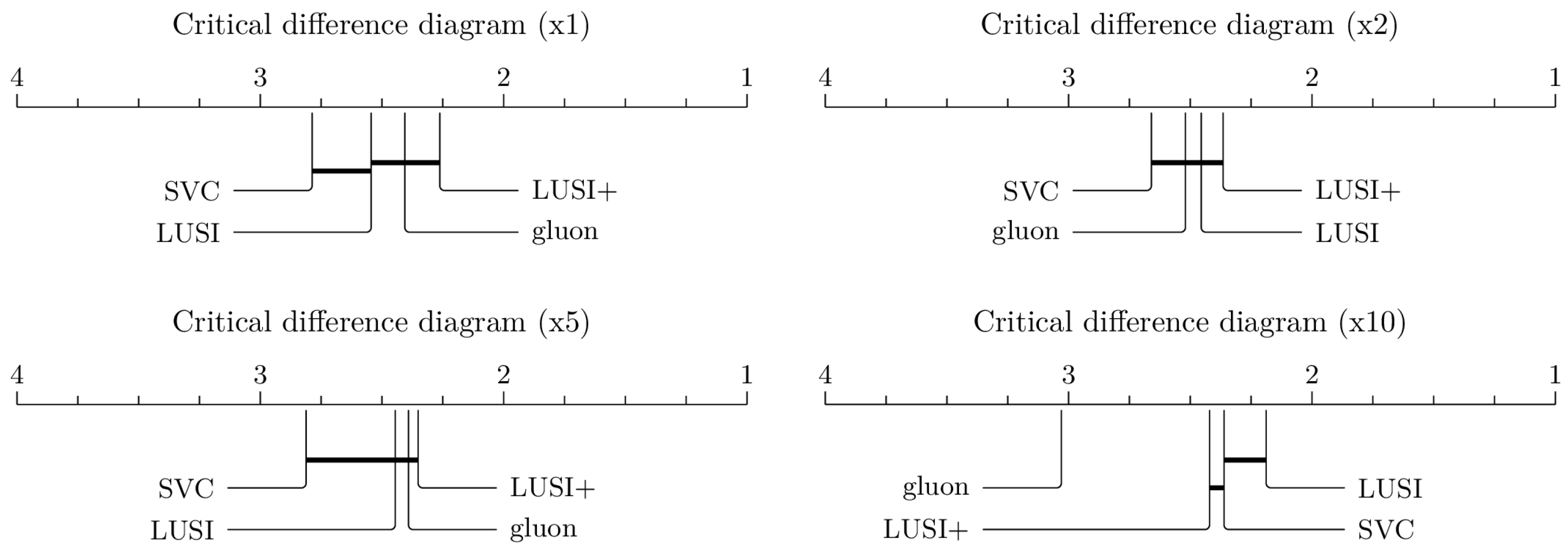
Furthermore, to assess the statistical significance of the differences in balanced accuracy between models, we performed an omnibus Friedman test, followed by a pairwise Wilcoxon signed-rank test with Holm correction, comparing every pair of methods at a 5% significance level, as outlined in [34]. This procedure determines whether there is evidence that the methods differ at all. The results of these tests are summarized in Figure 3. A solid line joining two models indicates that they are statistically indistinguishable at the 5% level.

5. Discussion of the Results

Figure 2 shows a high variance of the score for all models, which reflects the diversity and difficulty of the datasets, particularly in the most reduced runs.

The comparison between the LUSI family and AutoGluon matters most.

On the $\times 1$ run, the three models LUSI, LUSI+, and AutoGluon performed similarly, with AutoGluon edging out LUSI+ by a small margin. There was no evidence to distinguish these models statistically, although all three scored above the baseline SVC, as the first diagram in Figure 3 shows.

With respect to the $\times 2$ and $\times 5$ runs, all models performed similarly, with LUSI and LUSI+ beating AutoGluon on the $\times 5$ run. However, the differences were not statistically significant, as the diagrams in Figure 3 show.

In the $\times 10$ run, all models hovered around a score of 0.6; this indicates that tiny data is inherently difficult. AutoGluon performed poorly here, and the significance tests separated it from the other models. AutoGluon needs more time to fit its models than the cap allowed. On this matter, the LUSI family fit its models quickly, using less than a tenth of the runtime AutoGluon needed. The family remains slower than mature implementations such as SVC, refined over decades.

Furthermore, LUSI+ outperformed LUSI by a small margin in the first three runs; this indicates that adding invariants helped in some of the reduced versions of the datasets, supporting our hypothesis. The differences reached significance only in the $\times 10$ run, where LUSI scored above LUSI+.

Overall, the LUSI family of models performed better than expected, staying competitive with state-of-the-art classifiers. There is no statistical evidence to establish the superiority of the proposed model over the state of the art yet. However, we established that LUSI+ performed at least as well as AutoGluon on the evaluated datasets.

Possible improvements to alleviate the limitations of this reduced study include:

• A larger and more diverse dataset suite, which offers the statistical power to separate the models.
• More fitting time and tuned system defaults for AutoGluon. The 4-h AutoGluon run is the ceiling on the competitive benchmark TabArena [21].
• Improved preprocessing, hyperparameter tuning, and kernel selection for LUSI.
• A study of the role of the V matrix.
• Domain-specific predicates, although impractical in this study, to enhance both the performance and interpretability of the models.

Ablation studies and sensitivity analyses are needed to further understand the model’s behavior and performance.

6. Conclusions

We presented a family of classification models based on statistical learning theory. These models address the learning problem with convergence and generalization guarantees. We derived binary, multiclass, and multilabel classification algorithms. Moreover, we explored a new idea of using predicates to capture essential and domain-specific regularities that improve both the performance and interpretability of the models. This idea of statistical invariants complements the mathematical theory of learning by using the concept of weak convergence.

We ran a benchmark comparison of state-of-the-art classification models against the proposed models on a representative suite. The models performed well, staying on par with the state of the art; the results of this first implementation are promising.

Unlike black-box models, the LUSI family provides interpretable outputs, a proof of convergence to the global minimum, error bounds, and numerical stability. The empirical advantage of ensemble algorithms over mathematically grounded approaches such as LUSI challenges theoreticians and matters to practitioners.

Further research directions are: the discovery and analysis of useful general and domain-specific predicates, the exploration of kernels other than the Gaussian, and the computational challenges of model selection and numerical implementation.