Spike-Aware Propagation Approximation for Conductance-Based LIF Equations

Abstract

Large-scale spiking neural network simulation requires numerical integration that preserves membrane dynamics and spike timing without making fine-resolution updates prohibitively expensive. This balance is difficult for conductance-based leaky integrate-and-fire (LIF) networks because synaptic decay, threshold crossings, resets, and refractory periods form a hybrid dynamical system. To address this difficulty, we introduce a spike-aware propagation (SAP) approximation method that combines exact receptor-trace updates, analytic homogeneous membrane propagation, Gauss–Legendre quadrature, and spike localization, improving the accuracy–efficiency Pareto frontier. We establish an error bound and conditional convergence under consistent refinement for the proposed SAP. At h = 1 ms, the single-realization T = 1000 ms comparison showed a lower voltage RMSE for SAP than for Euler at the same width in the two high-activity regimes. The five-seed T = 200 ms robustness experiment likewise showed lower voltage RMSE for SAP than for NEST at the same width. At the highest drive, the paired mean reduction was 3.91 mV (95% CI, 3.85–3.97 mV). This quantified gain supports SAP as a practical route to an improved accuracy–efficiency balance in large-scale conductance-based LIF simulation while underscoring the method’s configuration-dependent and regime-dependent scope.

1. Introduction

Large-scale spiking neural network (SNN) simulation connects cellular dynamics with collective circuit behavior. Reduced point-neuron models make such studies computationally tractable, and the leaky integrate-and-fire (LIF) description offers a useful compromise between biophysical detail and numerical efficiency [1,2]. Conductance-based LIF models additionally retain receptor-specific decay and voltage-dependent synaptic driving forces that are absent from purely current-based descriptions [3]. These models support studies ranging from canonical recurrent circuits to data-constrained cortical- and brain-scale systems [4,5,6,7,8,9]. As network scale and biological scope increase, the neuronal update kernel is executed ever more frequently. Its numerical accuracy and efficiency therefore place direct limits on feasible simulation duration, parameter exploration, and network size.

The principal difficulty is that a conductance-based LIF network is a hybrid dynamical system, not merely a smooth ordinary differential equation (ODE). Receptor traces decay continuously between synaptic arrivals and jump when spikes arrive. The membrane voltage follows a non-autonomous linear ODE whose coefficients depend on those traces, while threshold crossings trigger resets and refractory clamps. Fine temporal resolution can track these mechanisms but requires repeated updates even when much of the state evolves predictably. Coarser resolution reduces this workload but may displace or miss a threshold crossing and delay its downstream effect. Because event timing changes later resets and synaptic inputs, a local error can propagate through the recurrent network. An effective integration strategy must therefore balance continuous voltage accuracy, discrete event timing, and computational efficiency.

Modern simulators improve throughput through parallel execution, code generation, graphics processing units (GPUs), and communication-aware spike delivery [10,11,12,13,14,15]. The accuracy available at a chosen temporal resolution nevertheless remains controlled by the neuronal integration and spike-detection scheme. Exact propagation is possible for time-invariant linear subthreshold systems [16], while off-grid methods improve spike timing within globally time-driven simulations [17,18]. Event-driven and retrospective tests provide accurate threshold handling for selected point-neuron models [19,20], and analytical conductance-based schemes exploit additional model structure [21,22]. These developments solve complementary parts of the problem, but combining exact receptor-trace updates, economical propagation under time-dependent conductance, and spike localization remains challenging in large recurrent networks.

Here, we develop a spike-aware propagation (SAP) approximation for conductance-based LIF networks under a shared scan and batched-delivery schedule. The principal contribution is a propagation kernel that keeps visible receptor traces and homogeneous attenuation exact while confining numerical quadrature to a smooth forcing integral and treating candidate crossings separately. We derive a conditional one-batch error estimate and test the method in million-neuron networks against Euler and NEST. Specifically, this paper (i) defines the SAP update and its event-handling conditions, (ii) separates quadrature and localization errors under a fixed itinerary, and (iii) identifies tested activity and parameter regimes in which SAP occupies useful accuracy–efficiency operating points. Section 2 positions SAP relative to existing integration strategies; Section 3 and Section 4 present the method and analysis; Section 5 and Section 6 report the experiments, limitations, and practical guidance.

2. Related Work

2.1. Large-Scale Spiking Network Models

Large-scale SNN models have progressively increased in both biological scope and data dependence. Early large recurrent and thalamocortical models established how neurons with reduced spiking can reproduce collective regimes that are difficult to study at the single-cell level [2,23]. Subsequent work integrated cell-type-specific connectivity into a full-scale cortical microcircuit [4], reconstructed neocortical microcircuitry in greater cellular detail [5], and linked local microcircuits across multiple macaque cortical areas [6]. Data-constrained mouse visual-cortex models extended this program by jointly using structural and functional measurements [7]. More recent brain-computing studies have pursued human-scale simulation and assimilation on large GPU systems [8,9]. These studies motivate numerical methods that remain economical when the same point-neuron update is executed many billions of times. The present work does not propose a new biological network architecture; it focuses on the integration kernel used to advance conductance-based LIF neurons within such large recurrent simulations.

2.2. Simulation Platforms and Scalability

General-purpose neural simulators balance model expressiveness, reproducibility, and performance in different ways [24]. NEURON and its optimized CoreNEURON engine support detailed neuronal models [25,26], whereas NEST targets large networks of point neurons with shared-memory and distributed parallelism [10]. Brian and Brian 2 use high-level model definitions and code generation to combine flexible specification with compiled execution [11,27]. NESTML extends this code-generation approach to portable descriptions of neuron and synapse models and makes the separation among model equations, event handling, and numerical integration explicit [28].

Hardware-oriented work has reduced the cost of both neuronal updates and spike delivery. GeNN generates accelerator-specific code for SNN simulation [12], while Brian2CUDA supplies a GPU backend for the Brian 2 model language [13]. Procedural connectivity reduces GPU memory pressure by generating connections when required [14], and NEST GPU studies have demonstrated both single-GPU and multi-GPU acceleration [29,30]. On distributed-memory systems, communication and data-structure optimizations have supported petascale and prospective exascale simulation [15,31,32]. Direct NEST–GeNN benchmarks further show that the preferable platform depends on model size, connectivity, hardware, and setup costs [33]. This body of work addresses where and how simulation workloads are executed. SAP is complementary: it changes the per-neuron propagation and threshold-localization procedure while retaining a shared scan schedule suited to parallel execution.

2.3. Time-Driven, Event-Driven, and Exact Integration

Numerical strategies for SNNs are commonly organized by how continuous flows and discrete spike events are scheduled. Globally time-driven methods update neuronal states on a shared grid and are straightforward to parallelize, but a grid-constrained threshold test quantizes spike times. Globally event-driven methods advance from one event to the next and can avoid inactive updates. However, they require reliable prediction of the next event and may introduce model-specific data structures. These are not mutually exclusive categories: hybrid schemes combine global time stepping with exact or off-grid operations within each step [24].

For linear, time-invariant subthreshold dynamics, matrix-exponential propagation gives an exact grid-to-grid update [16]. Morrison et al. combined exact subthreshold integration with continuous spike times in a discrete-time network schedule [17], and Hanuschkin et al. extended precise spike localization to nonlinear point-neuron models by iterative localization [18]. Event-driven algorithms have also been developed for nonlinear integrate-and-fire dynamics [19]. When a trajectory can cross and return below threshold between grid points, retrospective state-space tests can guarantee detection for selected linear subthreshold models [20]. Collectively, these methods show that exact propagation and accurate event timing can be combined with scalable scheduling. Their guarantees nevertheless depend on the subthreshold dynamics and on how incoming events are exposed to the neuron.

2.4. Conductance-Based Analytical Approximations

Conductance-based synapses are more difficult than current-based synapses because the synaptic input multiplies the membrane voltage. Brette developed an exact event-driven treatment for an integrate-and-fire model with exponential synaptic conductances under specific analytic restrictions [21]. Rudolph and Destexhe derived analytical conductance-based LIF models suited to event-driven strategies [22]. Related exact methods for exponential synaptic currents permit multiple time constants but apply to a different, current-based coupling structure [34]. Continued work on reduced conductance models, including simplified NMDA-receptor dynamics, illustrates the ongoing need to balance receptor detail and tractability [35].

SAP takes a different approximation route. It preserves the exponential decay and jumps of each visible receptor trace; therefore, no numerical ODE solver is required for those variables. The resulting membrane equation is treated by variation of constants: the homogeneous factor is evaluated analytically, and only the intractable forcing integral is approximated. This construction draws on the theory of exponential propagation and high-order Gaussian quadrature [36,37,38]. Threshold crossings and visible arrivals are then handled as explicit discontinuities, consistent with the general principle that a smooth solver must be coupled with event treatment for discontinuous ODE problems [39]. The distinction from the earlier conductance-based analytical schemes is therefore not that SAP makes the full hybrid trajectory exact. Rather, it isolates the approximation to a smooth integral and spike localization, which permits a direct decomposition of the resulting errors while retaining a common scan schedule for parallel execution.

The closest approaches differ from SAP in both model restrictions and event treatment. Exact subthreshold propagation and off-grid spike timing in globally time-driven simulations retain a shared network schedule but do not use SAP’s conductance-dependent forcing decomposition [16,17,18]. Brette’s exact conductance treatment and the analytical models of Rudolph and Destexhe exploit stronger model-specific structure in event-driven settings [21,22]. Retrospective state-space screening can provide perfect detection for selected linear subthreshold models [20], whereas SAP uses an endpoint screen whose completeness is an explicit condition. SAP therefore does not make the full hybrid trajectory exact. Its specific contribution is to combine exact visible receptor traces, analytic homogeneous attenuation, quadrature of only the residual forcing, and localized candidate crossings within a scan schedule suited to parallel batched delivery.

3. Methods

3.1. Conductance-Based LIF Equations

For neuron i, let $V_i\left(t\right)$ denote the membrane potential, $C_i$ the membrane capacitance, and $g_{L,i}$ the leak conductance. The leak, threshold, and reset potentials are $V_L$, $V_{\mathrm{th},i}$, and $V_{\mathrm{reset},i}$, respectively. The absolute refractory period is $T_{\mathrm{ref},i}$. The active receptor set is $\mathcal{U}=\{\mathrm{AMPA},{\mathrm{GABA}}_A\}$. For $u\in \mathcal{U}$, the receptor trace $J_i^u\left(t\right)$ has decay time ${\tau }_i^u$, conductance scale $g_i^u$, and reversal potential $V^u$. The synaptic weight from neuron j is $w_{ij}^u$, and the kth corresponding arrival occurs at $t_{ij}^{k,u}$.

With constant external drive $I_i$, the network dynamics are written in area-normalized units. Time is measured in $\mathrm{ms}$, voltage in $\mathrm{mV}$, capacitance density in $\mathsf{\mu }\mathrm{F}{\mathrm{cm}}^{-2}$, conductance density in $\mathrm{mS}{\mathrm{cm}}^{-2}$, and current density in $\mathsf{\mu }\mathrm{A}{\mathrm{cm}}^{-2}$. The traces $J_i^u$ and multipliers $w_{ij}^u$ are dimensionless.

$$\left\{\begin{array}{cc}\hfill C_i{\displaystyle \frac{\mathrm{d}{V}_i\left(t\right)}{\mathrm{d}t}}& =-\left(g_{L,i}+\sum _{u\in \mathcal{U}}{g}_i^u{J}_i^u\left(t\right)\right)V_i\left(t\right)+g_{L,i}{V}_L+\sum _{u\in \mathcal{U}}{g}_i^u{V}^u{J}_i^u\left(t\right)+I_i,\hfill \\ \hfill {\displaystyle \frac{\mathrm{d}{J}_i^u\left(t\right)}{\mathrm{d}t}}& =-{\displaystyle \frac{J_i^u\left(t\right)}{{\tau }_i^u}}+\sum _{j,k}{w}_{ij}^u\delta (t-t_{ij}^{k,u}),u\in \mathcal{U},\hfill \\ \hfill t_i^k& =inf\{t>t_i^{k-1}+T_{\mathrm{ref},i}:V_i\left(t\right)\ge V_{\mathrm{th},i}\},\hfill \\ \hfill V_i\left(t\right)& =V_{\mathrm{reset},i},t\in [t_i^k,t_i^k+T_{\mathrm{ref},i}].\hfill \end{array}\right..$$

(1)

Here, $\delta$ denotes the Dirac delta distribution. The membrane equation in (1) is equivalently expressed through the synaptic current $I_i^u\left(t\right)=g_i^u(V^u-V_i\left(t\right))J_i^u\left(t\right)$.

Let $[T_0,T_1]$ denote a batch-delivery interval of length $H=T_1-T_0$. The state at $T_0$ comprises the membrane potentials, the receptor traces, the refractory variables, and all presynaptic arrivals visible under the prescribed schedule. SAP scans the interval through common bins $[a,b]$ of width h, with a possibly shorter final bin. Although all neurons share this scan schedule, propagation for an individual neuron may begin within a bin when its refractory period ends. Under batched spike delivery, spikes emitted in $[T_0,T_1]$ enter the postsynaptic traces at $T_1$. Hence, H determines the delivery cadence, whereas h determines the grid used to identify candidate spikes.

3.2. Spike-Aware Propagation Approximation

Consider a predictor interval $[t_0,t]\subseteq [T_0,T_1]$, with $t>t_0$, on which the dynamics are smooth between visible arrivals. For $s\in [t_0,t]$, define

$$p_i\left(s\right)=g_{L,i}+\sum _{u\in \mathcal{U}}{g}_i^u{J}_i^u\left(s\right),q_i\left(s\right)=g_{L,i}{V}_L+\sum _{u\in \mathcal{U}}{g}_i^u{V}^u{J}_i^u\left(s\right)+I_i.$$

(2)

These coefficients reduce the subthreshold voltage dynamics to a scalar non-autonomous linear equation. Once the visible arrival set is fixed, the receptor traces can be updated exactly. Let ${\mathcal{A}}_i^u(t_0,t)=\{(j,k):t_0<t_{ij}^{k,u}\le t\}$ contain the index pairs for arrivals visible to neuron i through receptor u after the initial trace $J_i^u\left(t_0\right)$ has been formed. Then

$$J_i^u\left(t\right)=J_i^u\left(t_0\right)e^{-\eta /{\tau }_i^u}+\sum _{(j,k)\in {\mathcal{A}}_i^u(t_0,t)}{w}_{ij}^u{e}^{-(t-t_{ij}^{k,u})/{\tau }_i^u},\eta =t-t_0.$$

(3)

Equation (3) is exact for the prescribed visible arrivals. In the parallel implementation, spikes emitted during a batch are accumulated and become visible to postsynaptic traces at $T_1$. Propagation inside the batch therefore uses the visible-arrival set fixed at its left boundary.

Applying variation of constants to the membrane equation gives the following exact representation [16,37]:

$$V_i\left(t\right)=F_i(t,t_0)V_i\left(t_0\right)+{\int }_{t_0}^t{\displaystyle \frac{q_i\left(s\right)}{C_i}}{F}_i(t,s)ds,$$

(4)

where $F_i(t,s)=exp[-C_i^{-1}{\int }_s^t{p}_i\left(r\right)dr]$. On an arrival-free segment, $J_i^u\left(r\right)=J_i^u\left(s\right)e^{-(r-s)/{\tau }_i^u}$, and hence,

$$F_i(t,s)=exp\left[-{\displaystyle \frac{g_{L,i}}{C_i}}(t-s)-{\displaystyle \frac{1}{C_i}}\sum _{u\in \mathcal{U}}{g}_i^u{\tau }_i^u{J}_i^u\left(s\right)\left(1-e^{-(t-s)/{\tau }_i^u}\right)\right].$$

Visible arrivals partition the predictor interval into arrival-free segments, on each of which this propagator is exact. SAP therefore evaluates the homogeneous contribution analytically. Numerical approximation is confined to the inhomogeneous integral and spike localization.

SAP approximates the remaining integral with an M-node Gauss–Legendre rule on $[t_0,t]$ [38]:

$${\widehat{V}}_i(t;t_0)=F_i(t,t_0)V_i\left(t_0\right)+{\displaystyle \frac{\eta }{2}}{\displaystyle \sum _{m=1}^M}{\omega }_m{\displaystyle \frac{q_i\left(s_m\right)}{C_i}}{F}_i(t,s_m),s_m={\displaystyle \frac{t_0+t}{2}}+{\displaystyle \frac{\eta }{2}}{\xi }_m.$$

(5)

The nodes ${\left\{{\xi }_m\right\}}_{m=1}^M\subset [-1,1]$ are the roots of the degree-M Legendre polynomial, and ${\left\{{\omega }_m\right\}}_{m=1}^M$ are their associated Gauss–Legendre weights. Equation (5) approximates only the smooth forcing integral; receptor decay and homogeneous attenuation remain exact. The analysis assumes $0<h<{min}_i{T}_{\mathrm{ref},i}$ and the endpoint-screening condition of Theorem 1. On each active scan bin, the no-reset predictor must either remain subthreshold or possess one unique threshold zero followed by a suprathreshold right endpoint. The endpoint test then detects that crossing, while $h<T_{\mathrm{ref},i}$ prevents a second spike after the reset within the same bin. Within a bin $[a,b]$, neuron i remains clamped until $t_i^{\mathrm{eff}}=max\{a,t_i^{\mathrm{last}}+T_{\mathrm{ref},i}\}$. If $t_i^{\mathrm{eff}}<b$, Equation (5) propagates the neuron over $[t_i^{\mathrm{eff}},b]$ from traces decayed to $t_i^{\mathrm{eff}}$. Otherwise, the neuron remains clamped. A suprathreshold endpoint prediction marks a candidate spike, and the same predictor localizes its time within the bin. The localized spike time determines the next refractory release, and the bin-end voltage is reset. Because $h<T_{\mathrm{ref},i}$, the neuron cannot spike again in the unscanned remainder of that bin. Propagation resumes from the neuron-specific refractory release time in a later bin. Emitted spikes are accumulated and inserted into postsynaptic traces at $T_1$.

A smooth time-varying external drive can be included in $q_i\left(t\right)$ and evaluated within the same quadrature. Discontinuous or Poisson input events must instead be inserted into the visible-event partition. The experiments in Section 5 test constant drive only; validation under fluctuating input is left for future work.

Algorithm 1 summarizes the resulting SAP workflow. For each scan bin, it constructs refractory-aware initial states, advances the neurons with Equation (5), localizes candidate spikes, and accumulates emitted spikes for delivery at the batch boundary.

Figure 1 provides a compact view of the nested control flow that is easy to lose in pseudocode. It makes the inner scan-bin loop, conditional localization branch, batch-boundary delivery, and outer batch loop explicit; the distinct roles of H, h, and ${\epsilon }_t$ remain defined in the surrounding text and Algorithm 1.

Algorithm 1 SAP: spike-aware propagation approximation

Input:  States $V,J,t^{\mathrm{last}}$; neuronal parameters; final time T Batch length H; scan width $0<h<{min}_i{T}_{\mathrm{ref},i}$; quadrature order M; root tolerance ${\epsilon }_t$; iteration cap B Endpoint-screen completeness on every active bin, as specified in Theorem 1 Output:  Updated states $V,J,t^{\mathrm{last}}$, with emitted spikes delivered at batch boundaries   1: for each batch-delivery interval $[T_0,T_1]$ do   2:     Store $J\left(T_0\right)$ and initialize the outgoing counts $S\leftarrow 0$   3:     for each common scan bin $[a,b]\subseteq [T_0,T_1]$ of nominal width h do     Construct refractory-aware initial states   4:         for all neurons i do   5:            $t_i^{\mathrm{eff}}\leftarrow max\{a,t_i^{\mathrm{last}}+T_{\mathrm{ref},i}\}$ and ${\Delta }_i\leftarrow max\{0,b-t_i^{\mathrm{eff}}\}$   6:            $V_i^0\leftarrow V_{\mathrm{reset},i}$ if $t_i^{\mathrm{eff}}>a$; otherwise, $V_i^0\leftarrow V_i$   7:            Decay $J_i^u\left(T_0\right)$ to $J_i^{u,0}=J_i^u\left(t_i^{\mathrm{eff}}\right)$ for every receptor type u   8:            $V_i^{\mathrm{pred}}\leftarrow {\widehat{V}}_i(b;t_i^{\mathrm{eff}})$ if ${\Delta }_i>0$; otherwise, $V_i^{\mathrm{pred}}\leftarrow V_{\mathrm{reset},i}$   9:         end for     Detect and localize within-bin spikes 10:         Set $\mathcal{C}\leftarrow \{i:{\Delta }_i>0,V_i^{\mathrm{pred}}\ge V_{\mathrm{th},i}\}$ 11:         for all $i\in \mathcal{C}$ do 12:            With the same predictor, localize ${\widehat{t}}_i\in [t_i^{\mathrm{eff}},b]$ to tolerance ${\epsilon }_t$ or iteration cap B 13:            Set $t_i^{\mathrm{last}}\leftarrow {\widehat{t}}_i$, $S_i\leftarrow S_i+1$, and $V_i^{\mathrm{pred}}\leftarrow V_{\mathrm{reset},i}$ 14:         end for 15:         Accept $V_i\leftarrow V_i^{\mathrm{pred}}$ for every neuron 16:     end for 17:     Decay visible traces to $T_1$ and deliver the accumulated spike batch S 18: end for

4. Error Analysis

One-Batch Voltage-Error and Conditional Convergence Analysis

To isolate the propagation and spike-localization errors, fix one neuron i and one batch interval $[T_0,T_1]$. Let $V_i$ denote the exact voltage trajectory, and let ${\widehat{V}}_i$ denote the SAP trajectory. The two trajectories start from the same voltage, receptor traces, and refractory status at $T_0$, and they use the same prescribed visible-arrival data during the batch. Values at resets are taken right-continuously. A receptor trace jump at $T_1$ does not instantaneously change the voltage, and so the endpoint error is evaluated at $T_1^{-}$. This construction keeps the theorem focused on the observable membrane voltage while retaining the event times needed to control reset and refractory effects.

Let ${\mathcal{P}}_i$ be the collection of active predictor intervals obtained by cutting the scan bins at visible arrivals and refractory releases. Thus, every $K=[a_K,b_K]\in {\mathcal{P}}_i$ is smooth, $\left|K\right|\le h$, and ${\sum }_{K\in {\mathcal{P}}_i}\left|K\right|\le H$. For $a_K<x\le b_K$, define

$${\mathcal{G}}_{i,K}^{\left(2M\right)}=\underset{a_K<x\le b_K}{sup}{∥{\partial }_s^{2M}\left\{{\displaystyle \frac{q_i\left(s\right)}{C_i}}{F}_i(x,s)\right\}∥}_{L^{\infty }(a_K,x)},$$

(6)

and

$$d_{i,K}={\beta }_M{\left|K\right|}^{2M+1}{\mathcal{G}}_{i,K}^{\left(2M\right)},{\beta }_M={\displaystyle \frac{{(M!)}^4}{(2M+1){[\left(2M\right)!]}^3}}.$$

(7)

Theorem 1

(One-batch voltage error for spike-aware propagation). Fix $0<h<T_{\mathrm{ref},i}$ and an integer $B\ge 1$. Assume the following conditions on $[T_0,T_1]$.

1. 

The visible-arrival sequence is finite, and the functions in Equation (6) have bounded derivatives through order $2M$ on every $K\in {\mathcal{P}}_i$.

2. 

The exact and SAP trajectories remain in a bounded neighborhood with the same finite event itinerary. In particular, they have the same number and ordering of threshold crossings, resets, and refractory releases, and no such event coincides with a scan or batch boundary.

3. 

The endpoint screen is complete on this itinerary. On every active scan bin, either the SAP no-reset predictor remains below threshold throughout the bin, or it has exactly one threshold zero and is suprathreshold at the right endpoint. Every exact crossing has one corresponding predictor zero in a common initial bracket ${\mathcal{B}}_{i,\ell }\subseteq K_{i,\ell }$ of width ${\kappa }_{i,\ell }\le \left|K_{i,\ell }\right|\le h$.

4. 

Let ${\varphi }_{i,\ell }$ be the smooth unreset continuation of the exact pre-spike voltage on ${\mathcal{B}}_{i,\ell }$. Its threshold crossing ${\tau }_{i,\ell }$ is transversal, and

$${\displaystyle \frac{\mathrm{d}{\varphi }_{i,\ell }}{\mathrm{d}t}}\left(t\right)\ge {\gamma }_{i,\ell }>0,t\in {\mathcal{B}}_{i,\ell }.$$

The corresponding SAP predictor zero also lies in ${\mathcal{B}}_{i,\ell }$.

Let ${\mathcal{E}}_i$ index the crossings in the batch, and define the bisection remainder

$${\epsilon }_{i,\ell }^{\mathrm{bis}}=max\left\{{\epsilon }_t,{\kappa }_{i,\ell }{2}^{-B}\right\}.$$

(8)

Then, there exist constants ${\Lambda }_i^{\mathrm{q}}\ge 0$ and ${\Lambda }_i^{\mathrm{t}}\ge 0$ such that

$$\left|V_i\left(T_1^{-}\right)-{\widehat{V}}_i\left(T_1^{-}\right)\right|\le {\Lambda }_i^{\mathrm{q}}\sum _{K\in {\mathcal{P}}_i}{d}_{i,K}+{\Lambda }_i^{\mathrm{t}}\sum _{\ell \in {\mathcal{E}}_i}{\epsilon }_{i,\ell }^{\mathrm{bis}}.$$

(9)

The constants are uniform on the stated event-itinerary neighborhood. They depend on the model parameters, H, the transversality bounds and local flow sensitivities but not on h, ${\epsilon }_t$, or B. Here, ${\Lambda }_i^{\mathrm{q}}$ is dimensionless, whereas ${\Lambda }_i^{\mathrm{t}}$ has units of voltage per unit time.

If ${\mathcal{G}}_{i,K}^{\left(2M\right)}\le {\overline{\mathcal{G}}}_i^{\left(2M\right)}$ uniformly and ${max}_{\ell }{\epsilon }_{i,\ell }^{\mathrm{bis}}\le c_i{h}^{2M}$ along an itinerary-preserving refinement sequence, then

$$\left|V_i\left(T_1^{-}\right)-{\widehat{V}}_i\left(T_1^{-}\right)\right|\le \left[{\Lambda }_i^{\mathrm{q}}{\beta }_{M}H{\overline{\mathcal{G}}}_i^{\left(2M\right)}+{\Lambda }_i^{\mathrm{t}}{c}_i\#{\mathcal{E}}_i\right]h^{2M}.$$

(10)

Thus, the one-batch voltage error is $O\left(h^{2M}\right)$ under the stated refinement conditions.

Scope of Theorem 1. The estimate is conditional on a common finite event itinerary and complete endpoint screening. It does not cover spike insertion, deletion, or reordering, nor any within-bin crossing that returns below threshold before the right endpoint. Recurrent coupling can amplify these failures, which are assessed empirically rather than bounded by Theorem 1.

Proof. 

We first estimate the defect of one smooth predictor. Fix $K=[a_K,b_K]\in {\mathcal{P}}_i$ and $x\in (a_K,b_K]$. For an initial voltage v, the exact unreset flow is

$${\mathsf{\Phi }}_{i,K,x}\left(v\right)=F_i(x,a_K)v+{\int }_{a_K}^x{\displaystyle \frac{q_i\left(s\right)}{C_i}}{F}_i(x,s)\mathrm{d}s.$$

(11)

The SAP map replaces only the integral according to the M-node Gauss–Legendre rule,

$${\widehat{\mathsf{\Phi }}}_{i,K,x}\left(v\right)=F_i(x,a_K)v+{\displaystyle \frac{x-a_K}{2}}{\displaystyle \sum _{m=1}^M}{\omega }_m{\displaystyle \frac{q_i\left(s_{m,x}\right)}{C_i}}{F}_i(x,s_{m,x}),$$

(12)

where

$$s_{m,x}={\displaystyle \frac{a_K+x}{2}}+{\displaystyle \frac{x-a_K}{2}}{\xi }_m.$$

The Gauss–Legendre remainder formula [38] and $x-a_K\le \left|K\right|$ give

$$\left|{\mathsf{\Phi }}_{i,K,x}\left(v\right)-{\widehat{\mathsf{\Phi }}}_{i,K,x}\left(v\right)\right|\le d_{i,K}.$$

(13)

This estimate is uniform in x, and so it applies both to accepted endpoint updates and to predictor evaluations made during bisection.

If the exact and numerical segment maps start from different voltages v and $\widehat{v}$, then

$$\left|{\mathsf{\Phi }}_{i,K,x}\left(v\right)-{\widehat{\mathsf{\Phi }}}_{i,K,x}\left(\widehat{v}\right)\right|\le |F_i(x,a_K)\left|\right|v-\widehat{v}|+d_{i,K}.$$

(14)

On the bounded neighborhood in the theorem, $|F_i(x,a_K)|\le exp(L_i\left|K\right|)$ for some finite $L_i$. Products of these smooth propagation factors over the batch are therefore bounded by $exp\left(L_{i}H\right)$, independently of the number of scan intervals.

We next examine a threshold crossing using the standard smooth-event perturbation viewpoint [39]. Let ${\tau }_{i,\ell }$ be the zero of the exact unreset continuation ${\varphi }_{i,\ell }$, let ${\overline{\tau }}_{i,\ell }$ be the corresponding zero of the SAP predictor before bisection truncation, and let ${\widehat{\tau }}_{i,\ell }$ be the returned bisection time. Denote the uniform discrepancy between the exact unreset continuation and the numerical predictor on their common bracket by $r_{i,\ell }$. Because ${\varphi }_{i,\ell }\left({\tau }_{i,\ell }\right)=V_{\mathrm{th},i}$ and the SAP predictor equals $V_{\mathrm{th},i}$ at ${\overline{\tau }}_{i,\ell }$, transversality and the mean-value theorem yield

$$\begin{array}{cc}\hfill {\gamma }_{i,\ell }|{\overline{\tau }}_{i,\ell }-{\tau }_{i,\ell }|& \le |{\varphi }_{i,\ell }\left({\overline{\tau }}_{i,\ell }\right)-{\varphi }_{i,\ell }\left({\tau }_{i,\ell }\right)|\hfill \\ & =|{\varphi }_{i,\ell }\left({\overline{\tau }}_{i,\ell }\right)-V_{\mathrm{th},i}|\le r_{i,\ell }.\hfill \end{array}$$

(15)

This argument uses the smooth unreset continuation, not the physical voltage after its reset.

The retained bisection bracket contains ${\overline{\tau }}_{i,\ell }$. Its width is at most ${\epsilon }_t$ when the requested tolerance is reached and at most ${\kappa }_{i,\ell }{2}^{-B}$ when the iteration cap is reached. Hence,

$$|{\widehat{\tau }}_{i,\ell }-{\overline{\tau }}_{i,\ell }|\le {\epsilon }_{i,\ell }^{\mathrm{bis}},$$

(16)

and Equations (15) and (16) give

$$|{\widehat{\tau }}_{i,\ell }-{\tau }_{i,\ell }|\le {\displaystyle \frac{r_{i,\ell }}{{\gamma }_{i,\ell }}}+{\epsilon }_{i,\ell }^{\mathrm{bis}}.$$

(17)

It remains to propagate these defects through the batch with constants that do not grow with the number of scan intervals. Order the physical events in the common itinerary, and regard the intervening members of ${\mathcal{P}}_i$ as smooth stages. At a regular endpoint of a smooth stage, let $e_r$ be the voltage discrepancy and let ${\theta }_r$ be the magnitude of the crossing- or refractory-release-time discrepancy that is currently carried by the two trajectories; set ${\theta }_r=0$ when no such offset is active. Bounded derivatives of the flow on the itinerary-preserving neighborhood give uniform constants ${\overline{L}}_i,c_i,D_i\ge 0$ such that, for a smooth stage $K_r$ of length ${\Delta }_r=\left|K_r\right|$,

$$\begin{array}{cc}\hfill e_{r+1}& \le exp\left({\overline{L}}_i{\Delta }_r\right)e_r+c_i{\Delta }_r{\theta }_r+D_i{d}_{i,K_r},\hfill \end{array}$$

(18)

$$\begin{array}{cc}\hfill {\theta }_{r+1}& ={\theta }_r.\hfill \end{array}$$

(19)

Indeed, the first coefficient is the usual smooth-flow stability factor, and so $A_r\le exp({\overline{L}}_i|K_r|)$. The dependence on a displaced event endpoint enters through the vector field integrated over $K_r$; hence, its coefficient satisfies $B_r\le c_i|K_r|=O(|K_r\left|\right)$. The final term follows from Equation (14). These quantitative scalings are essential because the number of smooth stages may increase as h decreases.

Choose a fixed conversion factor ${\nu }_i>0$ with units of voltage per unit time. It converts the carried timing error into voltage units in the combined stability quantity $z_r=e_r+{\nu }_i{\theta }_r$; it does not change the numerical dynamics. Choose ${\tilde{L}}_i\ge max\{{\overline{L}}_i,c_i/{\nu }_i\}$. Since $e^x\ge 1+x$ for $x\ge 0$, Equations (18) and (19) imply

$$z_{r+1}\le exp\left({\tilde{L}}_i{\Delta }_r\right)z_r+D_i{d}_{i,K_r}.$$

(20)

Consequently, a discrete Gronwall inequality [37] or direct telescoping of Equation (20) over any consecutive smooth block $r=p,\dots ,q-1$ gives

$$z_q\le exp\left({\tilde{L}}_i{\displaystyle \sum _{r=p}^{q-1}}{\Delta }_r\right)\left(z_p+D_i{\displaystyle \sum _{r=p}^{q-1}}{d}_{i,K_r}\right).$$

(21)

The sum of all smooth-stage lengths in the batch is at most H. Thus, their combined amplification is at most $exp\left({\tilde{L}}_{i}H\right)$, independently of h and of the number of scan intervals.

We now separate the physical event maps from these smooth stages. The fixed event itinerary contains a finite number $J_i$ of visible-arrival jumps, crossing/reset pairs, and refractory releases; $J_i$ is independent of the scan partition. For a crossing event, uniform smooth-stage estimates on its common bracket and Equation (13) bound the predictor discrepancy by

$$r_{i,\ell }\le c_{i,\ell }^{\mathrm{pred}}{z}^{-}+D_{i,\ell }^{\mathrm{pred}}{d}_{i,K_{i,\ell }}.$$

Equation (17) then controls the new timing error. Both trajectories receive the same reset voltage, and the timing error is carried to the corresponding refractory release. At that release, boundedness of the vector field gives Lipschitz dependence of the restarted voltage on the release time. Visible-arrival jumps occur at the same prescribed times and are also locally Lipschitz. It follows that the jth physical event map satisfies

$$z_j^{+}\le Q_{i,j}{z}_j^{-}+R_{i,j}{d}_{i,K\left(j\right)}+{\mathbf{1}}_{\left\{j\mathrm{is}\mathrm{a}\mathrm{crossing}\right\}}{S}_{i,j}{\epsilon }_{i,\ell \left(j\right)}^{\mathrm{bis}},$$

(22)

where the defect term is taken as zero for an event with no associated predictor interval. The constants $Q_{i,j}$ and $R_{i,j}$ are dimensionless, whereas $S_{i,j}$ has units of voltage per unit time. They are uniform on the stated neighborhood: in particular, the factors ${\gamma }_{i,\ell }^{-1}$ from Equation (17) are bounded there.

Finally, telescope the alternating smooth-block estimates (21) and the $J_i$ event-map estimates (22). With

$$P_i=exp\left({\tilde{L}}_{i}H\right){\displaystyle \prod _{j=1}^{J_i}}max\{1,Q_{i,j}\},R_i^{*}=\underset{1\le j\le J_i}{max}{R}_{i,j},S_i^{*}=\underset{1\le j\le J_i}{max}{S}_{i,j},$$

where an empty maximum is zero, the common initial data $z_0=e_0+{\nu }_i{\theta }_0=0$ yield

$$e_{\mathrm{final}}\le z_{\mathrm{final}}\le P_i(D_i+R_i^{*})\sum _{K\in {\mathcal{P}}_i}{d}_{i,K}+P_i{S}_i^{*}\sum _{\ell \in {\mathcal{E}}_i}{\epsilon }_{i,\ell }^{\mathrm{bis}}.$$

(23)

The fixed finite event count, the total-length bound, and the uniform local coefficients show explicitly that neither multiplier depends on h, ${\epsilon }_t$, or B. Taking ${\Lambda }_i^{\mathrm{q}}=P_i(D_i+R_i^{*})$ and ${\Lambda }_i^{\mathrm{t}}=P_i{S}_i^{*}$ proves Equation (9).

Finally,

$$\sum _{K\in {\mathcal{P}}_i}{\left|K\right|}^{2M+1}\le h^{2M}\sum _{K\in {\mathcal{P}}_i}\left|K\right|\le H{h}^{2M}.$$

Combining this inequality with the uniform derivative bound and the assumed bisection scaling proves Equation (10).    □

Equation (9) is a conditional one-batch voltage estimate. It applies only when the initial data and event itinerary satisfy the stated conditions. Practical violations include grazing or non-transversal crossings, nearly coincident events, events at scan or batch boundaries, multiple crossings in one scan bin, and a crossing that returns below threshold before the endpoint screen. Strong recurrent input can also change the visible itinerary by inserting, deleting, or reordering spikes. The theorem does not bound these cases. Instead, the experiments below test the recurrent implementation directly and reveal the resulting non-monotone network-level errors.

5. Results and Discussion

5.1. Million-Neuron Network Experiments

We evaluated Euler, SAP, and NEST [10] across four constant-drive regimes. The current densities $I\in \{0.85,1,2,3\}\mathsf{\mu }\mathrm{A}{\mathrm{cm}}^{-2}$ produced same-input NEST reference firing rates of $9.16$, $14.69$, $57.97$, and $88.75\mathrm{Hz}$, respectively. These currents were selected as numerical stress regimes spanning weakly to strongly driven activity, not as an exhaustive set of biological states. All main comparisons retained the same three-solver suite, whereas the subsequent parameter sweeps varied SAP only. The complete configuration-level records are provided in Supplementary File S1.

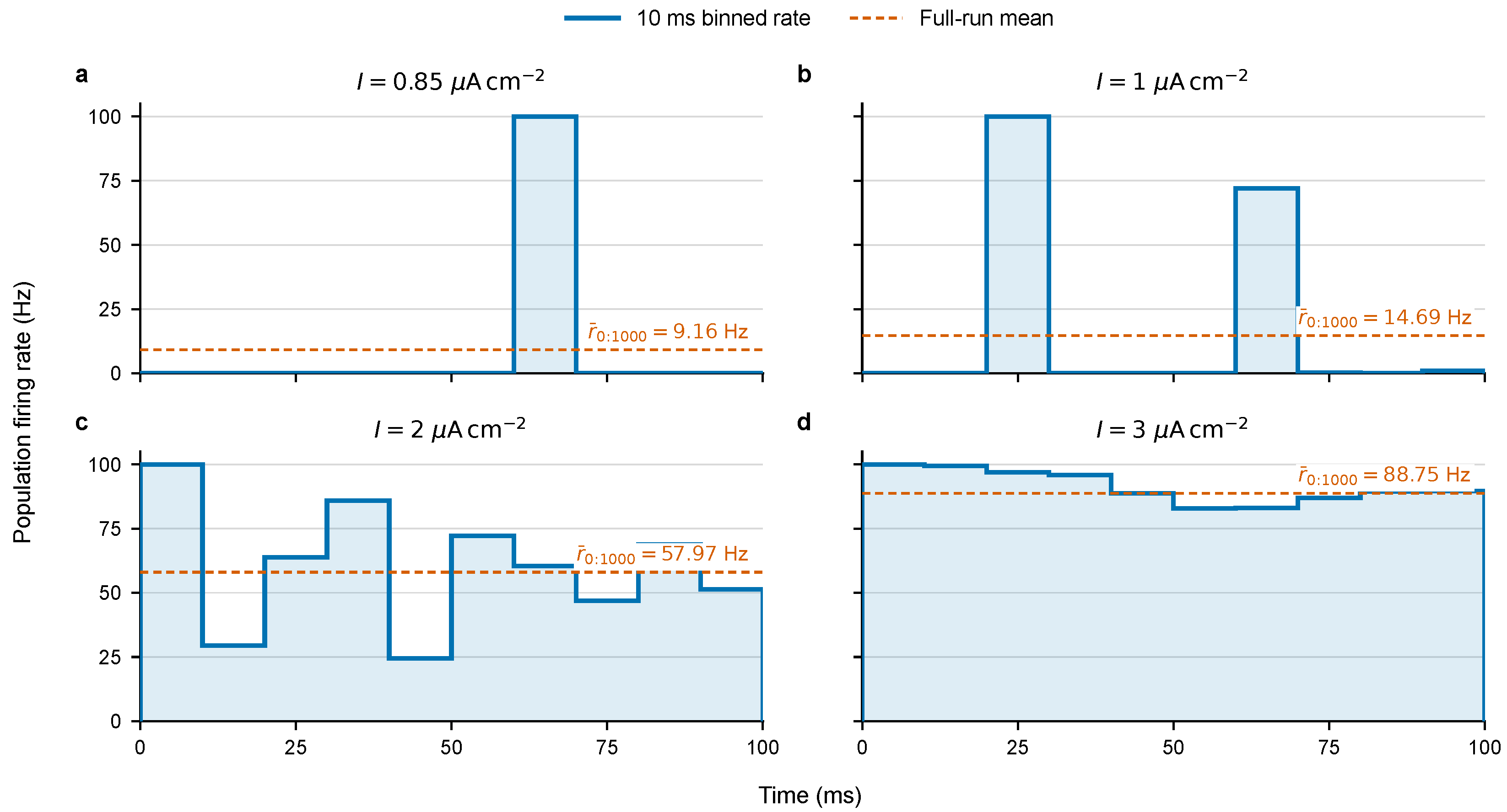
The sampled-neuron voltage trajectories examined below characterize threshold and reset timing for one neuron in the highest-drive regime; they do not establish population activity across all four regimes. We therefore report the corresponding population firing-rate traces from the fine-step NEST references in Figure 2.

The common axes in Figure 2 make the temporal distinction explicit. The two lower drives are intermittent during the initial $100\mathrm{ms}$, while every $10\mathrm{ms}$ bin is active at $I=2$ and $3\mathsf{\mu }\mathrm{A}{\mathrm{cm}}^{-2}$; the highest drive remains between $82.91$ and $100.00\mathrm{Hz}$ over this window. The experiment-wide dashed guides, rather than the value in any single transient bin, define the weak-to-strong regime ordering quoted above. These traces are a population-level diagnostic of the prespecified experiment.

5.1.1. Experimental Design and Evaluation Metrics

The topology, neuronal and synaptic parameters, external drive, initialization, and output-sampling grid were fixed across solver configurations. The experimental network contained $\mathrm{1,000,000}$ neurons, comprising $\mathrm{800,000}$ excitatory and $\mathrm{200,000}$ inhibitory neurons. Each neuron had fixed average in-degree $d=100$. The multiple-random-seed robustness experiments were conducted with a total simulation time of $T=200\mathrm{ms}$. Within each drive and run, NEST at $h=0.001\mathrm{ms}$ was the numerical reference, and the ordered set of $n_s$ sampled neurons was shared across solvers. The three accuracy–efficiency comparisons reported below pair error and ODE-solving-time centers from the main comparison with matched error and timing sample SDs from the robustness suite. These whiskers are descriptive, are not confidence intervals or empirical uncertainty estimates for the main comparison, and are not used for inference. Every simulation used a batch-delivery interval of $H=1\mathrm{ms}$ under one of four constant drives, $I\in \{0.85,1,2,3\}\mathsf{\mu }\mathrm{A}{\mathrm{cm}}^{-2}$.

The same fixed topology artifact was reused by every solver. Each target neuron received 100 distinct presynaptic neurons sampled without replacement, with self-connections excluded; the graph therefore contained neither autapses nor repeated source–target pairs. The first $\mathrm{800,000}$ source indices were excitatory and entered the AMPA channel, while the remaining $\mathrm{200,000}$ were inhibitory and entered the ${\mathrm{GABA}}_A$ channel. Each active connection used a fixed dimensionless multiplier $w_{ij}\sim \mathcal{U}[0,1)$ drawn during topology construction.

The area-normalized membrane parameters were $C_i=0.75\mathsf{\mu }\mathrm{F}{\mathrm{cm}}^{-2}$, $g_{L,i}=$1/30,000$\mathrm{S}{\mathrm{cm}}^{-2}$, and $V_L=-75\mathrm{mV}$. All neurons started at $V_i\left(0\right)=-57.5\mathrm{mV}$ with zero receptor traces and were not initially refractory. The threshold and reset potentials were $-50$ and $-65\mathrm{mV}$, respectively, and $T_{\mathrm{ref}}=5\mathrm{ms}$. AMPA and ${\mathrm{GABA}}_A$ had reversal potentials 0 and $-70\mathrm{mV}$ and decay times 2 and $10\mathrm{ms}$, respectively. Their base conductance densities were $g^{\mathrm{AMPA}}=1/55\mathrm{mS}{\mathrm{cm}}^{-2}$ and $g^{{\mathrm{GABA}}_A}=0.1\mathrm{mS}{\mathrm{cm}}^{-2}$, followed by the common scale $0.1$. Thus, a connection produced conductance-density increments $0.1g^{\mathrm{AMPA}}{w}_{ij}\mathrm{mS}{\mathrm{cm}}^{-2}$ and $0.1g^{{\mathrm{GABA}}_A}{w}_{ij}\mathrm{mS}{\mathrm{cm}}^{-2}$ in the two channels.

The NEST parameter conversion used an effective membrane area of ${10}^{-3}{\mathrm{cm}}^2$: $C_m=750\mathrm{pF}$, $g_L=100/3\mathrm{nS}$, and $I_e=1000I\mathrm{pA}$. The excitatory and inhibitory NEST connection weights were $+100g^{\mathrm{AMPA}}{w}_{ij}$ and $-100g^{{\mathrm{GABA}}_A}{w}_{ij}\mathrm{nS}$, respectively. The custom solvers stored voltage, receptor traces, quadrature data, and event times in double precision, while the sparse topology and weight arrays used single precision. Sampled voltage arrays were recorded in single precision.

The numerical settings varied only by solver and by the planned SAP ablations. Euler and SAP were implemented as graphics processing unit (GPU) solvers and were evaluated at $h\in \{1,0.1,0.01,0.001\}\mathrm{ms}$. The main SAP configuration used $M=2$, ${\epsilon }_t=0.01\mathrm{ms}$, and at most 15 bisection iterations. The ablations varied $M\in \{1,2,3,4\}$ and ${\epsilon }_t\in \{0.1,0.01,0.001\}\mathrm{ms}$. Every tested scan width satisfied $h<T_{\mathrm{ref}}=5\mathrm{ms}$. NEST 3.10.0-rc.2 used the iaf_cond_exp model with a $1\mathrm{ms}$ delay. All numerical comparisons used NEST at $h=0.001\mathrm{ms}$ as the reference under the matching drive and network realization.

Both suites were evaluated on a Dell Precision 7960 workstation with an Intel Xeon w5-3525 processor, 125 GiB of system memory, and three NVIDIA GeForce RTX 4090 GPUs (24 GiB each). GPU runs used one RTX 4090 and PyTorch 2.11.0 with CUDA 12.6; NEST ran on the same workstation with eight CPU threads. The three accuracy–efficiency comparisons reported below therefore compare one-GPU SAP/Euler with eight-thread CPU NEST and are not hardware-normalized benchmarks.

The interpretation of h depends on the solver. For SAP, h is the common scan width, although propagation may begin later within a bin when a refractory period ends. For NEST, h is the simulation resolution that bounds each interval advanced by the adaptive Runge–Kutta–Fehlberg $4\left(5\right)$ integrator in the GNU Scientific Library.

We quantified voltage accuracy by the sampled-neuron root mean square error (RMSE). We sampled $n_s=1000$ neurons at intervals of $\Delta s=1\mathrm{ms}$. Let $\mathcal{C}$ denote the resulting sampling grid and ${\mathcal{P}}_s$ the sampled-neuron set. For numerical voltage $V_{j,m}^{\mathrm{alg}}$ and reference voltage $V_{j,m}^{★}$, the metric is

$${\mathrm{RMSE}}_{V,\mathrm{sample}}={\left[{\displaystyle \frac{1}{\left|\mathcal{C}\right|}}\sum _{m\in \mathcal{C}}{\displaystyle \frac{1}{n_s}}\sum _{j\in {\mathcal{P}}_s}{\left(V_{j,m}^{\mathrm{alg}}-V_{j,m}^{★}\right)}^2\right]}^{1/2}.$$

(24)

We complemented voltage RMSE with two population spike-based quantities. Let $c_m^{\mathrm{alg}}$ and $c_m^{★}$ be the algorithm and reference population spike counts on the common sampling grid of width $\Delta s=1\mathrm{ms}$, and let $T_{\sec }$ denote the simulation duration expressed in seconds. The population firing rate and its absolute error are

$$r={\displaystyle \frac{1}{N{T}_{\sec }}}\sum _m{c}_m,\Delta r=|r_{\mathrm{alg}}-r_{★}|,$$

(25)

where N is the population size. For the population-count van Rossum quantity, the filtered counts satisfy $x_m=c_m+exp(-\Delta s/{\tau }_{\mathrm{VR}})x_{m-1}$ with ${\tau }_{\mathrm{VR}}=10\mathrm{ms}$. We report

$${\displaystyle \frac{D_{\mathrm{VR}}^{\mathrm{pop}}}{N}}={\displaystyle \frac{1}{N}}{\left[{\displaystyle \frac{\Delta s}{{\tau }_{\mathrm{VR}}}}\sum _m{\left(x_m^{\mathrm{alg}}-x_m^{★}\right)}^2\right]}^{1/2}.$$

(26)

This aggregate count-trace quantity is not a labeled-neuron spike-train distance.

For the robustness suite, we also retained neuron identity in the spike comparison. Let $c_{j,m}$ be the spike count of sampled neuron j in bin m, and let $x_{j,m}=c_{j,m}+exp(-\Delta s/{\tau }_{\mathrm{VR}})x_{j,m-1}$ with zero initial state. We calculated

$$d_j^2={\displaystyle \frac{\Delta s}{{\tau }_{\mathrm{VR}}}}\sum _m{\left(x_{j,m}^{\mathrm{alg}}-x_{j,m}^{★}\right)}^2,D_{\mathrm{VR},\mathrm{RMS}}^{\mathrm{lab}}={\left({\displaystyle \frac{1}{n_s}}{\displaystyle \sum _{j=1}^{n_s}}{d}_j^2\right)}^{1/2}.$$

(27)

This is a finite-horizon, $1\mathrm{ms}$ binned van Rossum count-trace distance with ${\tau }_{\mathrm{VR}}=10\mathrm{ms}$; the sum ends at the experiment-specific horizon T. It preserves the identities of the $n_s$ matched sampled neurons but neither resolves sub-millisecond event times nor includes the post-T exponential tail.

For the robustness suite, the independent statistical unit was one independently generated network realization ($n=5$ per solver–drive–width group). For a run-level quantity $Y_s$, we report the arithmetic mean and sample variance

$$s_Y^2={\displaystyle \frac{1}{n-1}}{\displaystyle \sum _{s=1}^n}{(Y_s-\overline{Y})}^2,{\mathrm{CI}}_{1-\alpha }=\overline{Y}\pm t_{1-\alpha /2,n-1}{\displaystyle \frac{s_Y}{\sqrt{n}}},$$

(28)

where $\alpha =0.05$ for the reported 95% intervals; with four degrees of freedom, the corresponding critical value is $2.7764$. The confidence intervals are pointwise and unadjusted. Direct method comparisons use the same calculation after forming within-run paired differences. The Supplementary Material reports the run-level observations and arithmetic mean ± sample-SD summaries. Voltage uncertainty is calculated from the n run-level RMSE values and remains in RMSE units. For the three accuracy–efficiency comparisons reported below, error groups are matched by solver, drive I (Imean), h, and metric, whereas timing groups are matched by solver, drive, and h. For the six firing-rate-error operating points with error center−SD below zero, the lower vertical arm is truncated at zero and the upper arm retains its full one-SD length.

To quantify reset-phase sensitivity, we recalculated voltage RMSE after excluding a sample whenever either compared voltage lay within ${10}^{-6}\mathrm{mV}$ of the $-65\mathrm{mV}$ reset plateau. We report the resulting RMSE together with the retained fraction of neuron–time samples.

For the three accuracy–efficiency comparisons reported below, the computational-cost coordinate is ode_solve_runtime_s. For Euler and NEST, it equals the recorded ode_update_runtime_s. The legacy SAP benchmark timed regular scan-bin endpoint propagation but excluded the predictor evaluations made during root bisection. We reconstructed a modeled bisection-inclusive SAP ODE-solving time as

$$t_{\mathrm{ODE}}=t_{\mathrm{scan}}\left(1+k_{\mathrm{bis}}{\widehat{N}}_{\mathrm{act}}/N_{\mathrm{bin}}\right),k_{\mathrm{bis}}=min\left\{B,max\left[1,⌈{log}_2\left(max\{h/{\epsilon }_t,1\}\right)⌉\right]\right\},$$

(29)

where $N_{\mathrm{bin}}=T/h$ and ${\widehat{N}}_{\mathrm{act}}=N_{\mathrm{bin}}[1-exp(-N_{\mathrm{spike}}/N_{\mathrm{bin}})]$ estimates active scan bins from the recorded population spike count. This reconstruction includes regular scan-bin and root-bisection predictor evaluations but excludes candidate-mask construction, bracket updates, stopping reductions, sparse synaptic delivery, recording, host transfer, and result writing. The NEST coordinate remains summed elapsed time over chunked nest.Simulate calls excluding voltage polling. Thus, the coordinate has a restricted computational scope and is not hardware neutral. The same reconstruction was applied to every matched robustness-suite SAP configuration before the horizontal sample SD was calculated.

5.1.2. Sampled-Neuron Voltage Dynamics

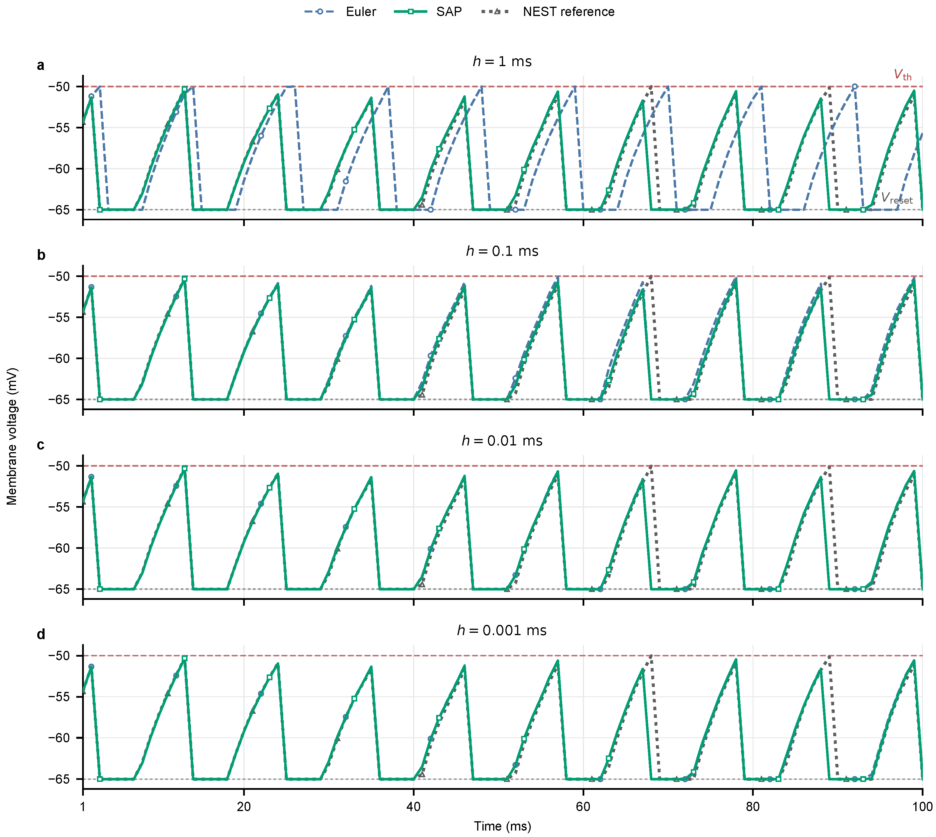
Before comparing aggregate error and cost, we examined the membrane-voltage trajectory of one sampled neuron. The intended comparison in Figure 3a–d is vertical across rows: Euler and SAP trajectories are shown as h decreases, while the same fine NEST reference remains fixed. The abrupt threshold-to-reset jumps make small horizontal event shifts appear as large pointwise voltage differences on the $1\mathrm{ms}$ recording grid. The figure uses the high-activity $I=3\mathsf{\mu }\mathrm{A}{\mathrm{cm}}^{-2}$ regime over the first $100\mathrm{ms}$.

At $h=1\mathrm{ms}$, the fixed trace shows several early reset events for which SAP and NEST are recorded at nearby sampling points, whereas Euler records the corresponding events later. The remaining rows show how the recorded Euler and SAP trajectories change as their step sizes are reduced. The repeated threshold approaches, abrupt resets, and $5\mathrm{ms}$ plateaus provide a qualitative illustration of the hybrid LIF dynamics for one prespecified neuron. The aggregate comparison below uses all $n_s$ sampled neurons over the complete simulation.

5.1.3. Accuracy–Efficiency Pareto Frontiers Across Activity Regimes

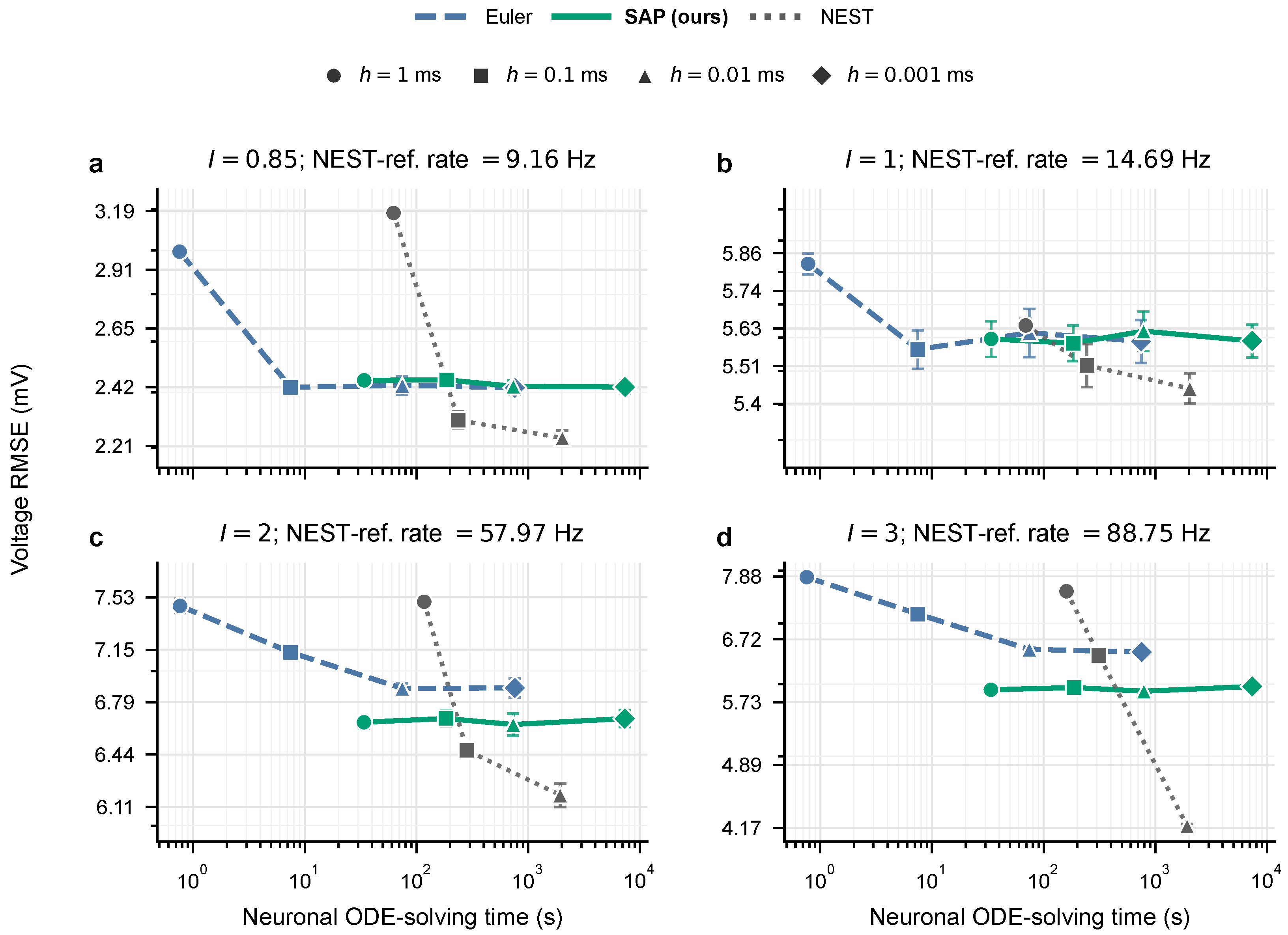
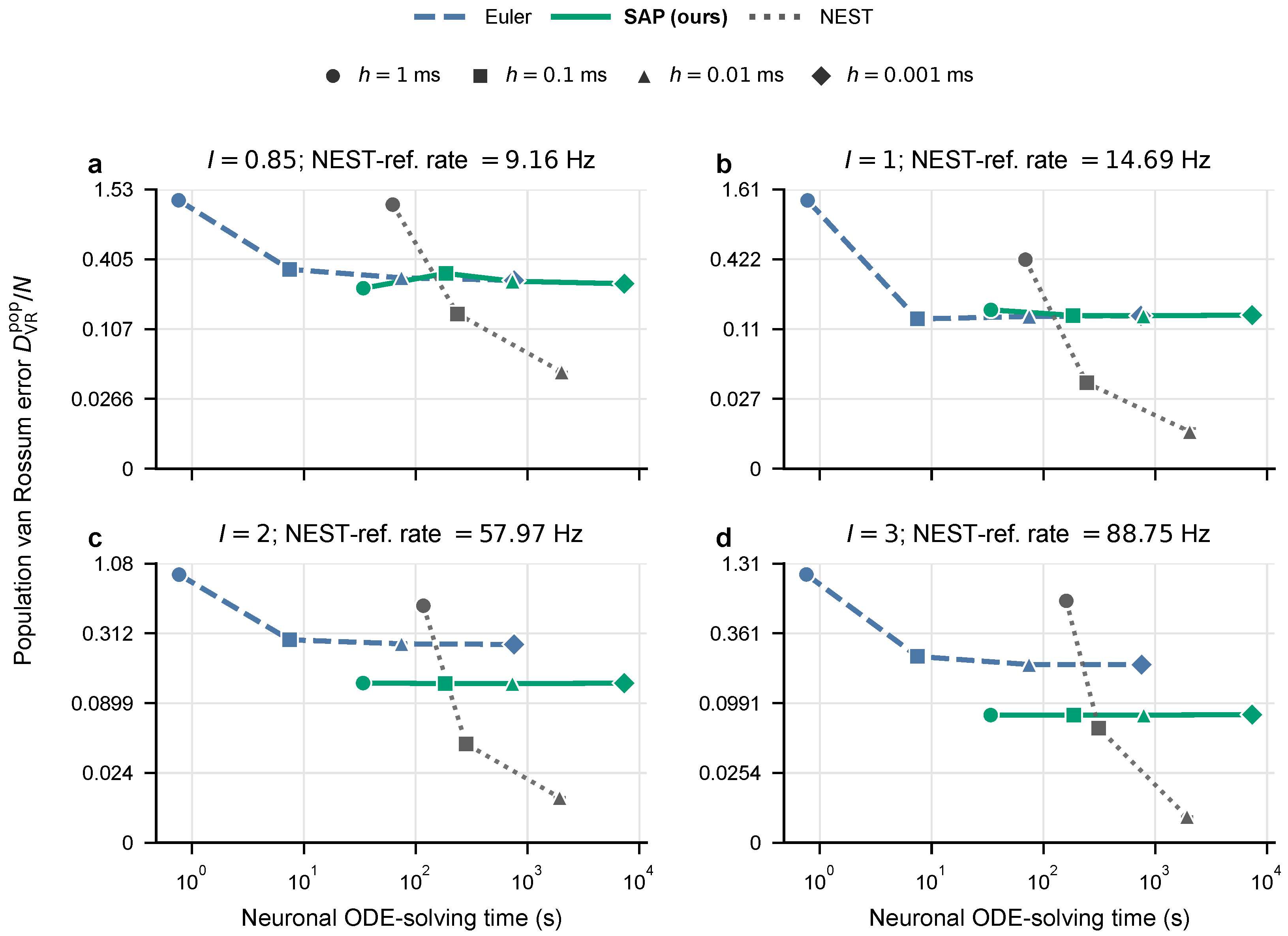
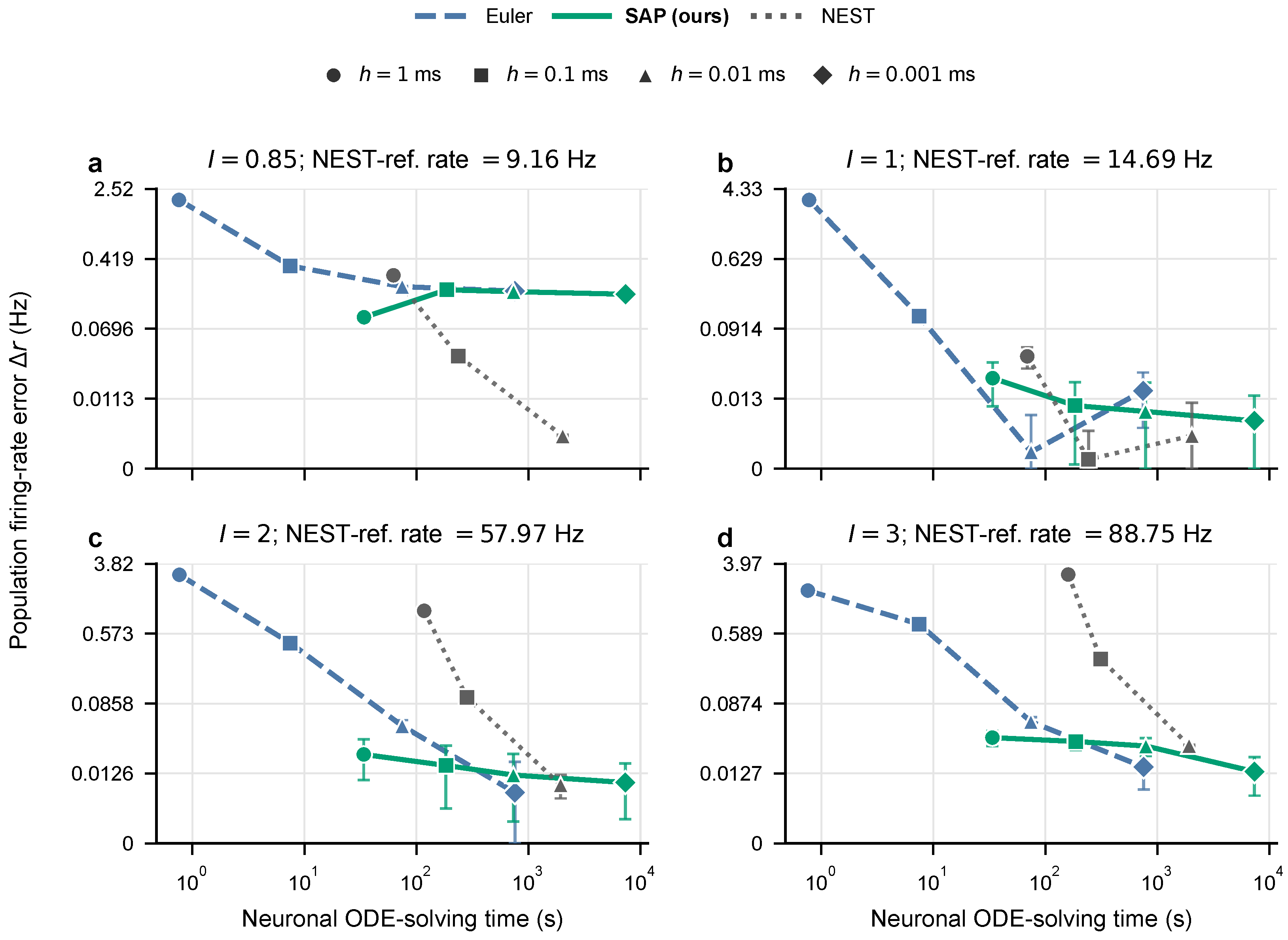
Figure 4, Figure 5 and Figure 6 compare three accuracy measures with a modeled bisection-inclusive neuronal ODE-solving coordinate in the main comparison. Every error is computed against the same-input NEST $h=0.001\mathrm{ms}$ numerical reference. The fine-NEST self-point is omitted because its error is zero. Centers and whiskers follow the provenance and matching rules in Section 5.1.1; neither whisker overlap nor separation is used for inference. The six Figure 6 points whose lower vertical arms would cross zero are truncated only at that physical boundary; their upper arms retain the full SD. Movement toward the lower left reduces the displayed error and modeled ODE-solving time, but the heterogeneous GPU/CPU timing contracts preclude hardware-neutral speedup claims.

At $h=1\mathrm{ms}$, SAP had lower voltage RMSE than same-width Euler and NEST in all four regimes. Relative to same-width NEST, the reductions were $0.85$ and $1.67\mathrm{mV}$ at $I=2$ and $3\mathsf{\mu }\mathrm{A}{\mathrm{cm}}^{-2}$. SAP’s modeled bisection-inclusive ODE-solving coordinate exceeded Euler’s but was below NEST’s. Because these coordinates mix GPU and CPU implementations and different timing contracts, this is a comparison of the tested operating points rather than a hardware-neutral speedup. The descriptive whiskers provide context only and do not alter this comparison.

At $h=1\mathrm{ms}$, SAP had lower population count-trace van Rossum error than same-width Euler and NEST in all four regimes. The ordering at finer widths depended on regime and comparator, and so the figure supports configuration-dependent rather than uniform dominance. Whisker overlap or separation is not used to support this ordering statement.

At $h=1\mathrm{ms}$, SAP had lower absolute population firing-rate error than same-width Euler and NEST in all four regimes. Fine-width comparisons remained metric- and regime-dependent, and the modeled timing contract prevents the interpretation of these coordinates as complete accuracy–cost dominance. The descriptive whiskers are not used to rank the methods.

Voltage RMSE need not decrease monotonically with h because the high-order estimate in Theorem 1 assumes a fixed event itinerary. Refinement can insert, delete, or reorder spikes and can shift resets relative to the fixed recording grid. Moreover, the batch-delivery interval remains $H=1\mathrm{ms}$ as h changes, leaving a separate network-level approximation. These hybrid and batched-delivery effects can dominate the shrinking smooth quadrature defect.

5.1.4. Robustness Across Independent Runs

The mean reference firing rates across the robustness-suite fine-NEST runs were $9.253\pm 0.013$, $16.715\pm 0.019$, $59.084\pm 0.033$, and $89.893\pm 0.011\mathrm{Hz}$ (mean ± sample SD). Run-level observations and group summaries treat each independently generated network realization as the statistical unit instead of treating neurons or time bins as independent replicates. The process-wall timing definition, results, and measurement limitations are reported only in Supplementary File S1.

Reset-phase displacement contributed materially to the voltage metric but did not account for it completely. For SAP at $h=1\mathrm{ms}$, the reset-excluded mean RMSEs were $0.647$, $2.638$, $2.529$, and $1.849\mathrm{mV}$ at the four drives, compared with all-sample means of $1.268$, $3.728$, $4.514$, and $3.603\mathrm{mV}$. These changes correspond to reductions of $49.0\%$, $29.3\%$, $44.0\%$, and $48.7\%$. The retained fractions were $0.950\pm 0.000$, $0.889\pm 0.002$, $0.637\pm 0.003$, and $0.503\pm 0.003$ (mean ± sample SD). Thus, disagreement near the reset plateau explains a substantial part of sampled-voltage RMSE, especially at higher activity, while the nonzero reset-excluded errors show that smooth-phase and event-itinerary differences remain.

Representative robustness-suite SAP group summaries are reported in Supplementary Table S9.

The most consistent joint improvement occurred in the matched coarse comparison at the two high drives. For SAP minus NEST at $h=1\mathrm{ms}$, the paired mean voltage-RMSE differences were $-2.145\mathrm{mV}$ (95% CI $[-2.225,-2.065]$) at $I=2$ and $-3.907\mathrm{mV}$ (95% CI $[-3.969,-3.845]$) at $I=3$. The corresponding labeled van Rossum differences were $-0.620$ (95% CI $[-0.636,-0.603]$) and $-0.975$ (95% CI $[-0.987,-0.962]$), while the firing-rate-error differences were $-1.041\mathrm{Hz}$ (95% CI $[-1.070,-1.012]$) and $-2.949\mathrm{Hz}$ (95% CI $[-2.960,-2.939]$). Every one of the five paired runs favored SAP on each metric. Supplementary Table S10 records the paired uncertainty and ordering counts instead of inferring a paired result from overlapping marginal intervals.

The robustness comparison with finer Euler did not replicate every main-comparison ordering. At $I=2$, SAP at $h=1\mathrm{ms}$ minus Euler at $h=0.01\mathrm{ms}$ gave paired differences of $+0.0275\mathrm{mV}$ for voltage RMSE (95% CI $[0.0031,0.0519]$), $+0.00628$ for labeled van Rossum RMS (95% CI $[0.00098,0.01158]$), and $+0.0454\mathrm{Hz}$ for firing-rate error (95% CI $[0.0370,0.0539]$); all five runs favored Euler on these three errors. At $I=3$, the voltage difference was $+0.0113\mathrm{mV}$ (95% CI $[-0.0108,0.0333]$), the labeled van Rossum difference was $+0.00441$ (95% CI $[-0.00130,0.01012]$), and the firing-rate-error difference was $+0.0711\mathrm{Hz}$ (95% CI $[0.0697,0.0726]$). In contrast, the aggregate population-count van Rossum metric favored SAP in all five runs at both drives. This disagreement is why the identity-preserving labeled metric is the primary spike-train result and why no universal cross-Euler superiority is claimed.

5.1.5. SAP Hyperparameter Ablations

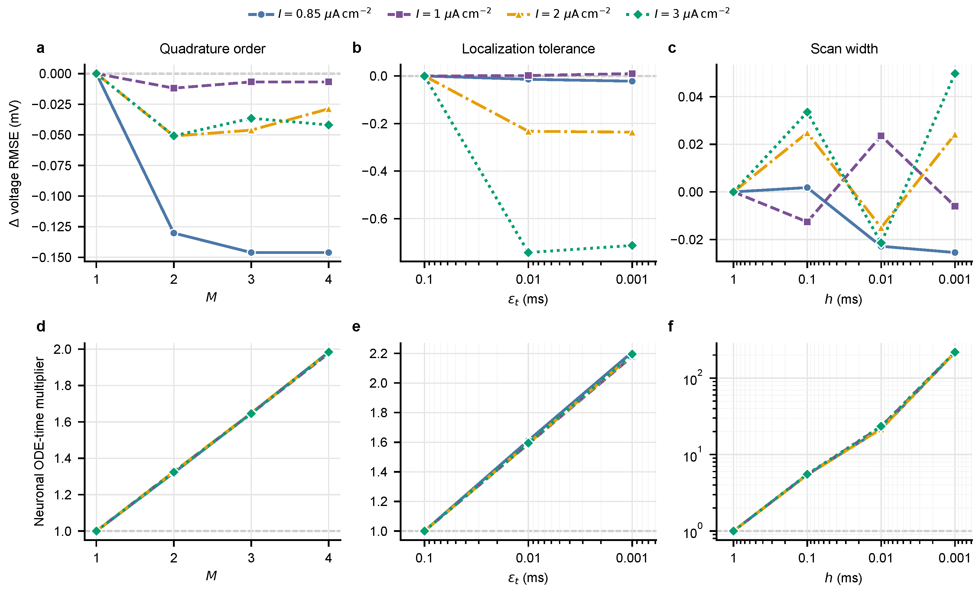
We next examined which SAP hyperparameters produced useful operating points using RMSE and pure ODE-solving time as the respective accuracy and efficiency metrics. The sweep separated the effects of quadrature order, spike-localization tolerance, and scan width.

Table 1. Quadrature-order ablation for SAP at $h=1\mathrm{ms}$ and ${\epsilon }_t=0.1\mathrm{ms}$, with at most five localization iterations. Each order reports sampled-voltage RMSE in $\mathrm{mV}$ and pure neuronal ODE-solving time in $\mathrm{s}$.

	$\mathit{M}=1$		$\mathit{M}=2$		$\mathit{M}=3$		$\mathit{M}=4$
$\mathit{I}$( $\mathsf{\mu }\mathbf{A}{\mathbf{cm}}^{\mathbf{-}\mathbf{2}}$)	RMSE	Time	RMSE	Time	RMSE	Time	RMSE	Time
$0.85$	$2.589$	$15.98$	$2.459$	$21.11$	$2.443$	$26.34$	$2.443$	$31.70$
1	$5.606$	$16.07$	$5.594$	$21.32$	$5.599$	$26.46$	$5.599$	$31.77$
2	$6.935$	$16.03$	$6.884$	$21.26$	$6.889$	$26.44$	$6.906$	$31.79$
3	$6.710$	$15.98$	$6.659$	$21.15$	$6.674$	$26.29$	$6.668$	$31.69$

and

Table 2. Spike-localization-tolerance ablation for $M=2$ SAP at $h=1\mathrm{ms}$. The $0.1\mathrm{ms}$ setting used at most five localization iterations; the tighter settings used at most 15. Each setting reports RMSE in $\mathrm{mV}$ and pure neuronal ODE-solving time in $\mathrm{s}$.

	${\mathit{\epsilon }}_{\mathit{t}}=0.1\mathbf{ms}$		${\mathit{\epsilon }}_{\mathit{t}}=0.01\mathbf{ms}$		${\mathit{\epsilon }}_{\mathit{t}}=0.001\mathbf{ms}$
$\mathit{I}$( $\mathsf{\mu }\mathbf{A}{\mathbf{cm}}^{\mathbf{-}\mathbf{2}}$)	RMSE	Time	RMSE	Time	RMSE	Time
$0.85$	$2.459$	$21.11$	$2.445$	$34.01$	$2.437$	$46.62$
1	$5.594$	$21.32$	$5.596$	$33.87$	$5.604$	$46.47$
2	$6.884$	$21.26$	$6.652$	$33.85$	$6.648$	$46.54$
3	$6.659$	$21.15$	$5.917$	$33.72$	$5.947$	$46.43$

report the $h=1\mathrm{ms}$ slices because they isolate the two local parameters at the coarsest tested scan width. The supplementary records contain all four scan widths. Figure 7 complements the absolute values in the tables by showing the accuracy change and ODE-solving-time multiplier relative to the coarsest setting in each sweep.

Increasing M from one to two reduced RMSE in all four regimes. This change increased pure ODE-solving time by approximately $32\%$, yielding an accuracy–efficiency trade-off rather than free improvement. Beyond $M=2$, the errors changed by at most $0.022\mathrm{mV}$ and were not consistently smaller. In particular, $M=4$ required approximately 49–$50\%$ more pure ODE-solving time than $M=2$. Its RMSE was equal or larger in three regimes, while at $I=0.85\mathsf{\mu }\mathrm{A}{\mathrm{cm}}^{-2}$ it improved RMSE by only $0.016\mathrm{mV}$. Thus, $M=2$ remained the practical compromise: it captured most of the order-dependent gain without moving to the high-cost, low-return end of the SAP frontier, as summarized in Figure 7a,d.

Tightening ${\epsilon }_t$ from $0.1$ to $0.01\mathrm{ms}$ reduced RMSE by $0.232\mathrm{mV}$ at $I=2\mathsf{\mu }\mathrm{A}{\mathrm{cm}}^{-2}$ and by $0.742\mathrm{mV}$ at $I=3\mathsf{\mu }\mathrm{A}{\mathrm{cm}}^{-2}$. The corresponding pure ODE-solving times increased by approximately $59\%$. The same tolerance change altered RMSE by only $-0.014$ and $+0.002\mathrm{mV}$ in the two lower-drive cases. Further tightening to $0.001\mathrm{ms}$ increased cost by another 37–$38\%$ without a consistent RMSE reduction. Hence, the tolerance sweep places ${\epsilon }_t=0.01\mathrm{ms}$ near the knee of the tested SAP frontier for the two high-activity regimes; the tighter setting buys little additional accuracy (Figure 7b,e).

Across the tested scan widths, the accuracy–efficiency ordering depended on the activity regime. For example, at $I=3\mathsf{\mu }\mathrm{A}{\mathrm{cm}}^{-2}$ with $M=2$ and ${\epsilon }_t=0.01\mathrm{ms}$, the RMSEs were $5.917$, $5.950$, $5.895$, and $5.967\mathrm{mV}$ as h decreased from 1 to $0.001\mathrm{ms}$. The associated pure ODE-solving time increased from $33.72$ to $7365\mathrm{s}$. At $I=0.85\mathsf{\mu }\mathrm{A}{\mathrm{cm}}^{-2}$, moving across the same settings changed the RMSE by only $0.025\mathrm{mV}$ while increasing pure ODE-solving time more than 200-fold. Thus, the lower-left operating points in this sweep were concentrated at intermediate or coarse settings (Figure 7c,f).

Figure 7 should therefore be read as a parameter-selection guide rather than a convergence plot: $M=2$ and ${\epsilon }_t=0.01\mathrm{ms}$ lie near the tested high-activity knee, while refining h is not monotonically beneficial in the recurrent hybrid system.

5.1.6. Discussion

Within the tested sweep, selected coarse SAP configurations produced useful sampled-voltage accuracy–efficiency points, particularly in the two higher-activity regimes. The quadrature-order and localization-tolerance ablations support $M=2$ and ${\epsilon }_t=0.01\mathrm{ms}$ as practical intermediate settings for those cases. The scan width remains regime dependent. Under the present metrics, SAP should not be described as uniformly preferable at $h\le 0.01\mathrm{ms}$ or in the two lower-activity regimes.

The robustness suite sharpens that boundary. Coarse SAP was consistently better than coarse NEST at the two higher drives under voltage RMSE, labeled and population binned van Rossum errors, and firing-rate error. However, its comparison with finer Euler depended on which spike representation was used: the aggregate population count and the identity-preserving sampled-neuron metric gave different orderings. Reporting both prevents a favorable population cancellation from being interpreted as labeled-neuron spike-time agreement.

The computational boundary is also structural. Storage for neuronal state and sparse connectivity scales as $O(N+E)$. Per batch, smooth SAP propagation requires approximately $O(MNH/h)$ work, while localization adds work proportional to the numbers of candidate spikes and bisection iterations. Synaptic delivery scales with the active edges.

In the main comparison at $h=1\mathrm{ms}$, SAP reduced all three errors relative to same-width Euler and NEST; its modeled bisection-inclusive ODE-solving coordinate was higher than Euler’s and lower than NEST’s. These observations support a configuration-dependent trade-off, not universal dominance or a hardware-neutral speedup. Replication of the primary NEST-inclusive sweep and fluctuating-input tests remain open validation tasks.

6. Conclusions

We introduced SAP for conductance-based LIF equations by combining exact visible receptor traces, analytic homogeneous propagation, Gauss–Legendre quadrature of the residual forcing, and localized candidate crossings. Under a prescribed visible-arrival schedule, complete endpoint screening, and a fixed bracketed transversal event itinerary, the analysis bounds one-batch voltage error and gives conditional convergence. In the main NEST-referenced comparison, coarse SAP reduced all three reported errors relative to same-width Euler and NEST in every activity regime; the heterogeneous modeled bisection-inclusive ODE-solving coordinate favored Euler over SAP but SAP over NEST. The ablations support $M=2$ and ${\epsilon }_t\approx 0.01\mathrm{ms}$ as practical intermediate settings for the tested high-activity cases. In the robustness suite, coarse SAP improved voltage RMSE, labeled-neuron binned van Rossum error, and firing-rate error relative to coarse NEST in every run at both higher drives. Comparisons with finer Euler were metric dependent and do not support uniform cross-resolution dominance.

Several limitations bound this conclusion. Both evaluations use constant external drive. The main-comparison findings lack empirical across-run uncertainty; the descriptive whiskers in Figure 4, Figure 5 and Figure 6 do not remove this limitation. Sampled-voltage RMSE is sensitive to reset-phase displacement, although reset-excluded RMSE shows that this is not the only source of error. The finite-horizon van Rossum quantities use $1\mathrm{ms}$ binned counts and do not measure sub-millisecond event times; the population-count metric also aggregates population counts and discards neuron identity. Figure 4, Figure 5 and Figure 6 use a modeled bisection-inclusive SAP ODE-solving coordinate that excludes data movement, sparse delivery, recording, and result writing. Comparisons with NEST also mix a GPU implementation with an eight-thread CPU simulator. Finally, the theorem excludes itinerary changes and incomplete endpoint screening, which can occur in recurrent simulations.

The next steps are to replicate the primary NEST-inclusive sweep with identity-preserving spike recording across additional independent runs, incorporate and extend Poisson/colored external-input protocols beyond the present constant-drive manuscript, and diagnose itinerary changes explicitly. These studies will determine how broadly the tested SAP operating points transfer beyond the present configuration.

References

1. Burkitt, A.N. A review of the integrate-and-fire neuron model: I. Homogeneous synaptic input. Biol. Cybern. 2006, 95, 1–19. [Google Scholar] [CrossRef] [Scilit]
2. Brunel, N. Dynamics of sparsely connected networks of excitatory and inhibitory spiking neurons. J. Comput. Neurosci. 2000, 8, 183–208. [Google Scholar] [CrossRef] [Scilit]
3. Destexhe, A.; Mainen, Z.F.; Sejnowski, T.J. Synthesis of models for excitable membranes, synaptic transmission and neuromodulation using a common kinetic formalism. J. Comput. Neurosci. 1994, 1, 195–230. [Google Scholar] [CrossRef] [Scilit]
4. Potjans, T.C.; Diesmann, M. The cell-type specific cortical microcircuit: Relating structure and activity in a full-scale spiking network model. Cereb. Cortex 2014, 24, 785–806. [Google Scholar] [CrossRef] [Scilit]
5. Markram, H.; Muller, E.; Ramaswamy, S.; Reimann, M.W.; Abdellah, M.; Sanchez, C.A.; Ailamaki, A.; Alonso-Nanclares, L.; Antille, N.; Arsever, S.; et al. Reconstruction and Simulation of Neocortical Microcircuitry. Cell 2015, 163, 456–492. [Google Scholar] [CrossRef] [Scilit]
6. Schmidt, M.; Bakker, R.; Shen, K.; Bezgin, G.; Diesmann, M.; van Albada, S.J. A multi-scale layer-resolved spiking network model of resting-state dynamics in macaque visual cortical areas. PLoS Comput. Biol. 2018, 14, e1006359. [Google Scholar] [CrossRef] [Scilit]
7. Billeh, Y.N.; Cai, B.; Gratiy, S.L.; Dai, K.; Iyer, R.; Gouwens, N.W.; Abbasi-Asl, R.; Jia, X.; Siegle, J.H.; Olsen, S.R.; et al. Systematic integration of structural and functional data into multi-scale models of mouse primary visual cortex. Neuron 2020, 106, 388–403.e18. [Google Scholar] [CrossRef] [Scilit]
8. Lu, W.; Zeng, L.; Wang, J.; Xiang, S.; Qi, Y.; Zheng, Q.; Xu, N.; Feng, J. Imitating and exploring the human brain’s resting and task-performing states via brain computing: Scaling and architecture. Natl. Sci. Rev. 2024, 11, nwae080. [Google Scholar] [CrossRef] [Scilit]
9. Lu, W.; Du, X.; Wang, J.; Zeng, L.; Ye, L.; Xiang, S.; Zheng, Q.; Zhang, J.; Xu, N.; Feng, J.; et al. Simulation and assimilation of the digital human brain. Nat. Comput. Sci. 2024, 4, 890–898. [Google Scholar] [CrossRef] [Scilit]
10. Gewaltig, M.O.; Diesmann, M. NEST (NEural Simulation Tool). Scholarpedia 2007, 2, 1430. [Google Scholar] [CrossRef] [Scilit]
11. Stimberg, M.; Brette, R.; Goodman, D.F.M. Brian 2, an intuitive and efficient neural simulator. eLife 2019, 8, e47314. [Google Scholar] [CrossRef] [Scilit]
12. Yavuz, E.; Turner, J.; Nowotny, T. GeNN: A code generation framework for accelerated brain simulations. Sci. Rep. 2016, 6, 18854. [Google Scholar] [CrossRef] [Scilit]
13. Alevi, D.; Stimberg, M.; Sprekeler, H.; Obermayer, K.; Augustin, M. Brian2CUDA: Flexible and efficient simulation of spiking neural network models on GPUs. Front. Neuroinform. 2022, 16, 883700. [Google Scholar] [CrossRef] [Scilit]
14. Knight, J.C.; Nowotny, T. Larger GPU-accelerated brain simulations with procedural connectivity. Nat. Comput. Sci. 2021, 1, 136–142. [Google Scholar] [CrossRef] [Scilit]
15. Jordan, J.; Ippen, T.; Helias, M.; Kitayama, I.; Sato, M.; Igarashi, J.; Diesmann, M.; Kunkel, S. Extremely scalable spiking neuronal network simulation code: From laptops to exascale computers. Front. Neuroinform. 2018, 12, 2. [Google Scholar] [CrossRef] [Scilit]
16. Rotter, S.; Diesmann, M. Exact digital simulation of time-invariant linear systems with applications to neuronal modeling. Biol. Cybern. 1999, 81, 381–402. [Google Scholar] [CrossRef] [Scilit]
17. Morrison, A.; Straube, S.; Plesser, H.E.; Diesmann, M. Exact subthreshold integration with continuous spike times in discrete-time neural network simulations. Neural Comput. 2007, 19, 47–79. [Google Scholar] [CrossRef] [Scilit]
18. Hanuschkin, A.; Kunkel, S.; Helias, M.; Morrison, A.; Diesmann, M. A general and efficient method for incorporating precise spike times in globally time-driven simulations. Front. Neuroinform. 2010, 4, 113. [Google Scholar] [CrossRef] [Scilit]
19. Tonnelier, A.; Belmabrouk, H.; Martinez, D. Event-driven simulations of nonlinear integrate-and-fire neurons. Neural Comput. 2007, 19, 3226–3238. [Google Scholar] [CrossRef] [Scilit]
20. Krishnan, J.; Porta Mana, P.; Helias, M.; Diesmann, M.; Di Napoli, E. Perfect detection of spikes in the linear sub-threshold dynamics of point neurons. Front. Neuroinform. 2018, 11, 75. [Google Scholar] [CrossRef] [Scilit]
21. Brette, R. Exact simulation of integrate-and-fire models with synaptic conductances. Neural Comput. 2006, 18, 2004–2027. [Google Scholar] [CrossRef] [Scilit]
22. Rudolph, M.; Destexhe, A. Analytical integrate-and-fire neuron models with conductance-based dynamics for event-driven simulation strategies. Neural Comput. 2006, 18, 2146–2210. [Google Scholar] [CrossRef] [Scilit]
23. Izhikevich, E.M.; Edelman, G.M. Large-scale model of mammalian thalamocortical systems. Proc. Natl. Acad. Sci. USA 2008, 105, 3593–3598. [Google Scholar] [CrossRef] [Scilit]
24. Brette, R.; Rudolph, M.; Carnevale, T.; Hines, M.; Beeman, D.; Bower, J.M.; Diesmann, M.; Morrison, A.; Goodman, P.H.; Harris, F.C.; et al. Simulation of networks of spiking neurons: A review of tools and strategies. J. Comput. Neurosci. 2007, 23, 349–398. [Google Scholar] [CrossRef] [Scilit]
25. Hines, M.L.; Carnevale, N.T. The NEURON simulation environment. Neural Comput. 1997, 9, 1179–1209. [Google Scholar] [CrossRef] [Scilit]
26. Kumbhar, P.; Hines, M.; Fouriaux, J.; Ovcharenko, A.; King, J.; Delalondre, F.; Schuermann, F. CoreNEURON: An optimized compute engine for the NEURON simulator. Front. Neuroinform. 2019, 13, 63. [Google Scholar] [CrossRef] [Scilit]
27. Goodman, D.; Brette, R. Brian: A simulator for spiking neural networks in Python. Front. Neuroinform. 2008, 2, 5. [Google Scholar] [CrossRef] [Scilit]
28. Linssen, C.; Babu, P.N.; Eppler, J.M.; Koll, L.; Rumpe, B.; Morrison, A. NESTML: A generic modeling language and code generation tool for the simulation of spiking neural networks with advanced plasticity rules. Front. Neuroinform. 2025, 19, 1544143. [Google Scholar] [CrossRef] [Scilit]
29. Golosio, B.; Tiddia, G.; De Luca, C.; Pastorelli, E.; Simula, F.; Paolucci, P.S. Fast simulations of highly-connected spiking cortical models using GPUs. Front. Comput. Neurosci. 2021, 15, 627620. [Google Scholar] [CrossRef] [Scilit]
30. Tiddia, G.; Golosio, B.; Albers, J.; Senk, J.; Simula, F.; Pronold, J.; Fanti, V.; Pastorelli, E.; Paolucci, P.S.; van Albada, S.J. Fast simulation of a multi-area spiking network model of macaque cortex on an MPI–GPU cluster. Front. Neuroinform. 2022, 16, 883333. [Google Scholar] [CrossRef] [Scilit]
31. Thibeault, C.M.; Minkovich, K.; O’Brien, M.J.; Harris, F.C.; Srinivasa, N. Efficiently passing messages in distributed spiking neural network simulation. Front. Comput. Neurosci. 2013, 7, 77. [Google Scholar] [CrossRef] [Scilit]
32. Kunkel, S.; Schmidt, M.; Eppler, J.M.; Plesser, H.E.; Masumoto, G.; Igarashi, J.; Ishii, S.; Fukai, T.; Morrison, A.; Diesmann, M.; et al. Spiking network simulation code for petascale computers. Front. Neuroinform. 2014, 8, 78. [Google Scholar] [CrossRef] [Scilit]
33. Schmitt, F.J.; Rostami, V.; Nawrot, M.P. Efficient parameter calibration and real-time simulation of large-scale spiking neural networks with GeNN and NEST. Front. Neuroinform. 2023, 17, 941696. [Google Scholar] [CrossRef] [Scilit]
34. Brette, R. Exact simulation of integrate-and-fire models with exponential currents. Neural Comput. 2007, 19, 2604–2609. [Google Scholar] [CrossRef] [Scilit]
35. Skaar, J.E.W.; Haug, N.; Plesser, H.E. A simplified model of NMDA-receptor-mediated dynamics in leaky integrate-and-fire neurons. J. Comput. Neurosci. 2025, 53, 475–487. [Google Scholar] [CrossRef] [Scilit]
36. Moler, C.; Van Loan, C. Nineteen dubious ways to compute the exponential of a matrix, twenty-five years later. SIAM Rev. 2003, 45, 3–49. [Google Scholar] [CrossRef] [Scilit]
37. Hochbruck, M.; Ostermann, A. Exponential integrators. Acta Numer. 2010, 19, 209–286. [Google Scholar] [CrossRef] [Scilit]
38. Trefethen, L.N. Is Gauss quadrature better than Clenshaw–Curtis? SIAM Rev. 2008, 50, 67–87. [Google Scholar] [CrossRef] [Scilit]
39. Dieci, L.; Lopez, L. A survey of numerical methods for IVPs of ODEs with discontinuous right-hand side. J. Comput. Appl. Math. 2012, 236, 3967–3991. [Google Scholar] [CrossRef] [Scilit]
Figure 1. SAP control flow. At the start of each batch [ T 0 , T 1 ] , SAP stores the visible trace state and initializes the outgoing spike counts. In each scan bin [ a , b ] , it constructs refractory-aware states, exactly decays visible receptor traces, predicts active-neuron endpoint voltages using the analytic homogeneous propagator and M-node Gauss–Legendre quadrature, and forms the candidate set C = { i : Δ i > 0 , V i pred ( b ) V th , i } . If C is nonempty, bisection localizes and registers its spikes before all bin-end states are committed; inactive neurons remain clamped at reset. Explicit decisions repeat the scan-bin loop to T 1 , deliver the accumulated spikes, and advance the outer batch loop. The stated endpoint-completeness condition and h < T ref , i exclude an undetected return below threshold and a second spike within one scan bin.
Axioms 15 00632 g001
Figure 2. Population firing-rate traces across four million-neuron activity regimes. Panel (a) shows the regime at I = 0.85 μ A cm 2 ; panel (b), I = 1 μ A cm 2 ; panel (c), I = 2 μ A cm 2 ; and panel (d), I = 3 μ A cm 2 . Each panel shows the first 100 ms of the prespecified, N = 10 6 fine-step NEST iaf_cond_exp reference ( h = 0.001 ms ) at the indicated constant drive. Each step is the population spike count c in one non-overlapping 10 ms bin divided by N × 0.010 s ; no smoothing was applied, and all panels use identical axes. Orange dashed lines denote the experiment-wide mean reference rates of 9.16 , 14.69 , 57.97 , and 88.75 Hz . Because all neurons shared the prescribed initial voltage, the lower-drive traces retain synchronized initial-condition transients, whereas the two higher drives sustain population firing throughout the displayed window.
Axioms 15 00632 g002
Figure 3. Sampled-neuron membrane-voltage trajectories during the first 100 ms of the million-neuron network experiment at I = 3 μ A cm 2 . Panel (a) compares Euler and SAP at h = 1 ms ; panel (b), at h = 0.1 ms ; panel (c), at h = 0.01 ms ; and panel (d), at h = 0.001 ms . NEST uses the fixed h = 0.001 ms reference configuration in every row. SAP used M = 2 , ε t = 0.01 ms , and at most 15 localization iterations. Markers are displayed at selected common recording times, and lines connect all values recorded on the 1 ms grid. Horizontal guides identify the threshold and reset voltages. All curves use the common experimental configuration. SAP denotes spike-aware propagation.
Axioms 15 00632 g003
Figure 4. Sampled-voltage accuracy–ODE-solving time operating points across four million-neuron activity regimes. Panel (a) reports the regime at I = 0.85 μ A cm 2 ; panel (b), at I = 1 μ A cm 2 ; panel (c), at I = 2 μ A cm 2 ; and panel (d), at I = 3 μ A cm 2 . Errors use same-input NEST at h = 0.001 ms as the numerical reference; its firing rate is shown in each title. Centers show the main-comparison error and ODE-solving time values; vertical and horizontal whiskers show the matched error and reconstructed ODE-solving time sample SDs from the robustness suite (Section 5.1.1). The whiskers are descriptive overlays and are not used for inference. Marker shape identifies h, and lines connect tested operating points only for visualization. The fine-NEST self-point is omitted because its error against itself is zero. Both axes are logarithmic; ordinate tick labels are given directly in mV, without a redundant scientific multiplier when the values are naturally expressed as ordinary decimals. The abscissa is ode_solve_runtime_s. For SAP, the recorded scan-propagation benchmark is scaled by the configured bisection iterations and estimated active-bin fraction, thereby including modeled root-bisection predictor evaluations; Euler and NEST retain their recorded update timings. Sparse delivery, recording, host transfer, and result writing remain excluded, and the NEST coordinate is summed chunked-Simulate time excluding voltage polling. SAP denotes spike-aware propagation.
Axioms 15 00632 g004
Figure 5. Population count-trace van Rossum error versus modeled neuronal ODE-solving time. Errors use same-input NEST at h = 0.001 ms as the numerical reference; the regimes, symbols, connecting lines, and timing contract otherwise match Figure 4. Panel (a) reports the regime at I = 0.85 μ A cm 2 ; panel (b), at I = 1 μ A cm 2 ; panel (c), at I = 2 μ A cm 2 ; and panel (d), at I = 3 μ A cm 2 . Centers show the main-comparison error and ODE-solving time values; vertical and horizontal whiskers show the matched error and reconstructed ODE-solving time sample SDs from the robustness suite (Section 5.1.1). They are descriptive overlays and are not used for inference. The ordinate is the finite-horizon 1 ms binned population metric D VR pop / N of Equation (26), with τ VR = 10 ms and no post-T tail; it is not a labeled-neuron event-time distance. To retain zero as a physical boundary, the ordinate uses the monotone zero-anchored transform g ( y ) = asinh ( y / s ) , where the common method-neutral scale is s = 0.10 times the pooled median of all displayed non-reference values. Ticks remain in the original units, and the abscissa is logarithmic.
Axioms 15 00632 g005
Figure 6. Absolute population firing-rate error Δ r versus modeled neuronal ODE-solving time. Errors use same-input NEST at h = 0.001 ms as the numerical reference; the regimes, symbols, connecting lines, and timing contract otherwise match Figure 4. Panel (a) reports the regime at I = 0.85 μ A cm 2 ; panel (b), at I = 1 μ A cm 2 ; panel (c), at I = 2 μ A cm 2 ; and panel (d), at I = 3 μ A cm 2 . Centers show the main-comparison error and ODE-solving time values; vertical and horizontal whiskers show the matched error and reconstructed ODE-solving time sample SDs from the robustness suite (Section 5.1.1). For the six points where center−SD is negative, the lower whisker arm is truncated at the physical zero boundary, while the upper arm retains its full one-SD length. The whiskers are descriptive overlays and are not used for inference. The monotone zero-anchored ordinate g ( y ) = asinh ( y / s ) uses the same method-neutral plotting rule as Figure 5: s = 0.10 times the pooled median of all displayed non-reference values, with tick labels in hertz. The abscissa is logarithmic.
Axioms 15 00632 g006
Figure 7. Relative effects of SAP hyperparameters across the four constant-drive regimes. Panel (a) reports the change in sampled-voltage RMSE as quadrature order M varies; panel (b) reports the change in RMSE as localization tolerance ε t varies; panel (c) reports the change in RMSE as scan width h varies; panel (d) reports the pure ODE-solving-time multiplier as M varies; panel (e) reports this multiplier as ε t varies; and panel (f) reports this multiplier as h varies. The quadrature-order sweep uses h = 1 ms , ε t = 0.1 ms , and at most five localization iterations. The localization-tolerance sweep uses M = 2 and h = 1 ms ; the 0.1 ms setting used at most five iterations, whereas the tighter settings used at most 15. The scan-width sweep uses M = 2 , ε t = 0.01 ms , and at most 15 iterations. Negative RMSE changes indicate improved accuracy relative to the coarsest setting of each sweep. All connected points use the same prespecified experimental realization. SAP denotes spike-aware propagation.
Axioms 15 00632 g007