A Unified Hybrid Estimation Strategy Using Multiple Auxiliary Transformations in Systematic Sampling with Simulation and Real-Life Applications

Abstract

Estimating the finite population mean under systematic sampling becomes challenging when auxiliary information is nonlinear, skewed, or structurally complex, as conventional linear estimators often lose efficiency. This study proposes a new class of weighted hybrid estimators that combine harmonic and geometric transformations of the auxiliary variable. The proposed approach is designed to capture nonlinear relationships while handling skewed data and reducing sensitivity to extreme observations. Expressions for bias and mean squared error are derived, and optimal weights are obtained by minimizing the mean squared error. The theoretical results indicate that the proposed estimators are more efficient than traditional ratio, product, regression, and exponential-type estimators. A simulation study further confirms their improved performance across various population structures, correlation levels, and sampling fractions, with notable improvements in skewed and nonlinear settings. The proposed class provides a flexible and reliable alternative for practical applications in systematic sampling.

1. Introduction

The estimation of finite population parameters is a fundamental topic in survey sampling theory, with the population mean being one of the most commonly used and practically important measures. Since the early development of sampling methodologies, considerable attention has been devoted to developing estimators that maintain high accuracy under practical survey conditions. In this regard, both the sampling design and the estimator structure play crucial roles in determining efficiency, particularly when auxiliary information is available.

Systematic sampling is a widely used probability sampling method, particularly suitable for populations that are naturally ordered or geographically arranged. In this approach, a random starting point is selected, and the remaining units are chosen at fixed intervals from the population list. Compared with simple random sampling, systematic sampling is easier to implement and can yield higher precision when the population follows a smooth pattern or exhibits slight trends. However, the performance of estimators under this design depends heavily on the underlying population structure, as hidden patterns or ordering effects may influence the accuracy of the results.

Systematic sampling has long been recognized as a practical alternative to simple random sampling, particularly for large and well-structured populations where ease of implementation and uniform coverage are essential. Early theoretical contributions by [1,2] established the probabilistic foundation of systematic sampling and highlighted its applicability in large-scale survey investigations. Subsequently, Kish [3] demonstrated that the variance of the systematic sample mean is highly influenced by population ordering and structural trends, in contrast to simple random sampling. This characteristic distinguishes systematic sampling from simple random sampling and underscores the importance of selecting appropriate estimators under such designs. Further theoretical and methodological developments in systematic sampling can be found in [4,5,6,7].

The auxiliary information has long played an important role in mean estimation for improving efficiency. Ratio and product estimators, which were initially designed under the assumption of simple random sampling by [8], were subsequently generalized to systematic sampling by several researchers, such as [9,10,11,12]. These estimators can reduce variance when the auxiliary variable is strongly correlated with the study variable; however, their performance deteriorates when these assumptions are violated. Later research demonstrated that even better performance could be achieved using regression-type estimators, which explicitly capture linear relationships, although they are more sensitive to model misspecification. Generalized and regression-type estimators were further introduced by [13] to enhance estimation efficiency, and it is important to note that these estimator structures are adaptable. Further developments include nonlinear transformations, such as difference-, product-, and ratio-mean-based estimators, which were proposed to improve robustness and flexibility, including the methods suggested by [14]. Several researchers have made important contributions to the development of efficient estimators under the systematic sampling scheme. For instance, Singh et al. (1998) [15] introduced almost unbiased ratio- and product-type estimators to improve estimation accuracy, while Singh et al. (2011) [16] proposed modified ratio and product estimators to enhance efficiency when auxiliary information is available. In subsequent work, Singh et al. (2012) [17] and Singh et al. (2013) [18] introduced a broader class of estimators for the population mean under systematic sampling, demonstrating improved efficiency over existing methods. Later, Tailor et al. [19] proposed a ratio-cum-product estimator that combines the advantages of both ratio and product approaches, resulting in better performance for certain types of populations. More recently, Khan et al. [20] developed a chain ratio-type estimator to further refine mean estimation within the same framework.

A number of studies have also focused on weighted and transformed estimators in systematic sampling and related settings. For instance, References [21,22] presented modified ratio-type estimators based on auxiliary information and reported improved performance under appropriate conditions. In a similar direction, References [23,24,25,26] proposed enhanced ratio, exponential, and difference-type estimators by utilizing additional characteristics of the auxiliary variable, such as its minimum and maximum values. Recent studies have continued to expand the scope of efficient estimation methods in systematic sampling by introducing memory-based, weighted, and difference-type approaches. For example, Koçyiğit [27] proposed new memory-type estimators designed to improve the estimation of the population mean under systematic sampling. Similarly, Karim et al. [28] investigated the estimation and monitoring of the population mean through an exponentially weighted moving average scheme, demonstrating the usefulness of combining systematic sampling with adaptive weighting techniques. In another contribution, Pal et al. [29] developed an efficient difference estimator for finite population mean estimation and showed its improved performance compared with existing estimators. More recently, Nagy et al. [30] extended the application of memory-type estimators to time-scaled surveys, further highlighting the growing importance of auxiliary information and adaptive estimation strategies in systematic sampling.

Despite these advances, limited attention has been given to hybrid estimators that simultaneously use harmonic and geometric transformations within the context of systematic sampling. This gap motivates the present study, which proposes a new class of weighted mean estimators based on a unified transformation framework. The bias and mean squared error are derived using first-order approximations, and the efficiency comparisons indicate that the proposed estimators perform better than several existing methods.

1.1. Scope, Objectives, and Contributions of the Proposed Estimators

Existing estimators under systematic sampling mainly rely on ratio, product, regression, or single-transformation approaches based on auxiliary information. However, limited work has been conducted on hybrid transformation-based estimators that combine harmonic, geometric, and power-type adjustments within a unified systematic sampling framework. In addition, many existing estimators are primarily designed for relatively simple linear population structures and may show reduced efficiency when the auxiliary variable follows nonlinear or skewed distributions.

Motivated by this research gap, the present study proposes a new class of weighted hybrid estimators for estimating the finite population mean under systematic sampling. The proposed framework combines harmonic and geometric-type transformations of the auxiliary variable to improve estimation efficiency under different population structures.

The main objectives and contributions of this study are summarized as follows:

• To develop new hybrid estimators under systematic sampling using multiple transformation forms of auxiliary information within a unified estimation framework.
• To derive approximate expressions for the bias and mean squared error of the proposed estimators using first-order approximations.
• To obtain the optimal values of the unknown constants by minimizing the mean squared error expressions.
• To examine the performance of the proposed estimators under linear, nonlinear, skewed, and periodic population structures through simulation experiments.
• To compare the proposed estimators with existing classical estimators under systematic sampling using both simulated and real population data.
• To investigate the efficiency behavior of hybrid transformation-based estimators under complex population structures and different correlation settings.

The proposed methodology is intended to provide a flexible alternative for practical survey applications where auxiliary information is available and the population structure may deviate from standard linear assumptions.

1.2. Potential Applications of the Proposed Methodology

The proposed estimators may be useful in practical survey applications where systematic sampling and auxiliary information are commonly employed. Possible application areas include agricultural surveys, environmental studies, public health investigations, economic surveys, and industrial quality control studies. These applications often involve ordered or structured populations in which nonlinear or skewed auxiliary variables may arise, making hybrid transformation-based estimation approaches potentially beneficial.

2. Notations

Consider a finite population denoted by $W=(W_1,W_2,W_3,\dots ,W_N),$ consisting of N distinct units. These units are indexed from 1 to N according to a fixed ordering. Let T denote the study variable and V represent the auxiliary variable. Unless stated otherwise, it is assumed that the population size satisfies $N=nk$, where n and k are positive integers. Under this assumption, the population can be partitioned into k systematic samples, each containing n units.

One systematic sample is selected at random from the k possible samples, and observations on both the study variate t and the auxiliary variate v are recorded for all units in the selected sample. Let $(t_{ij},v_{ij})$ denote the observed values corresponding to the jth unit in the ith systematic sample, where $i=1,2,\dots ,k$ and $j=1,2,\dots ,n$. The systematic sample means are defined as

$${\overline{t}}_{sy}={\displaystyle \frac{1}{n}}{\displaystyle \sum _{j=1}^n}{t}_{ij},{\overline{v}}_{sy}={\displaystyle \frac{1}{n}}{\displaystyle \sum _{j=1}^n}{v}_{ij}.$$

These estimators are unbiased for the corresponding population means $\overline{T}$ and $\overline{V}$, respectively. It is further assumed that the population mean $\overline{V}$ of the auxiliary variable V is known.

The variability of the study variable t and the auxiliary variable v within the population is measured through their respective population variances. In addition, the linear association between t and v is quantified by their population covariance. These quantities are defined as follows:

$$S_t^2={\displaystyle \frac{1}{N-1}}{\displaystyle \sum _{i=1}^N}{(t_i-\overline{T})}^2,$$

$$S_v^2={\displaystyle \frac{1}{N-1}}{\displaystyle \sum _{i=1}^N}{(v_i-\overline{V})}^2$$

and

$$S_{tv}={\displaystyle \frac{1}{N-1}}{\displaystyle \sum _{i=1}^N}(t_i-\overline{T})(v_i-\overline{V}),$$

respectively. We define the square of the coefficients of variations of t and v as follows:

$$C_t^2={\displaystyle \frac{S_t^2}{{\overline{T}}^2}},C_v^2={\displaystyle \frac{S_v^2}{{\overline{V}}^2}}.$$

Furthermore, let ${\rho }_t$ and ${\rho }_v$ be inter-class correlations between two units in the systematic sample for the study variate t and auxiliary variate v, respectively. These are determined as:

$${\rho }_t={\displaystyle \frac{E\left(t_{ij}-\overline{T}\right)\left(t_{i{j}^{\prime }}-\overline{T}\right)}{E{\left(t_{ij}-\overline{T}\right)}^2}},{\rho }_v={\displaystyle \frac{E\left(v_{ij}-\overline{V}\right)\left(v_{i{j}^{\prime }}-\overline{V}\right)}{E{\left(v_{ij}-\overline{V}\right)}^2}}.$$

The correlation coefficient between $(t,v)$ is expressed as:

$${\rho }_{tv}={\displaystyle \frac{E\left(t_{ij}-\overline{T}\right)\left(v_{ij}-\overline{V}\right)}{\sqrt{E{\left(t_{ij}-\overline{T}\right)}^{2}E{\left(v_{ij}-\overline{V}\right)}^2}}}.$$

Now, we introduce the subsequent error components along with the remaining symbols. Define the error terms as:

$${\overline{t}}_{sy}=\overline{T}(1+{\zeta }_0),{\overline{v}}_{sy}=\overline{V}(1+{\zeta }_1),$$

where

$${\zeta }_0={\displaystyle \frac{{\overline{t}}_{sy}-\overline{T}}{\overline{T}}},{\zeta }_1={\displaystyle \frac{{\overline{v}}_{sy}-\overline{V}}{\overline{V}}},$$

such that

$$E\left({\zeta }_0\right)=E\left({\zeta }_1\right)=0.$$

In addition,

$$E\left({\zeta }_0^2\right)=\theta C_t^2{D}_t,E\left({\zeta }_1^2\right)=\theta C_v^2{D}_v,E\left({\zeta }_0{\zeta }_1\right)=\theta \sqrt{D_{tv}}{\rho }_{tv}{C}_t{C}_v,$$

where

$$D_t=\left[1+(n-1){\rho }_t\right],$$

$$D_v=\left[1+(n-1){\rho }_v\right],$$

$$D_{tv}={\displaystyle \frac{D_t}{D_v}}=\left[{\displaystyle \frac{1+(n-1){\rho }_t}{1+(n-1){\rho }_v}}\right],$$

$$F_{tv}={\rho }_{tv}\left({\displaystyle \frac{C_t}{C_v}}\right)$$

and

$$\theta ={\displaystyle \frac{N-1}{nN}}.$$

3. Existing Estimators

In this section, several existing estimators under systematic sampling are briefly discussed, as they provide an important foundation for the present study. These estimators are later used to compare the performance and efficiency of the proposed estimators.

The sampling variance, which is also the mean squared error, of the usual unbiased estimator ${\overline{t}}_{sy}$ under systematic sampling when auxiliary information is not used is defined as:

$$\mathrm{MSE}\left({\overline{t}}_{sy}\right)=\theta {\overline{T}}^2{D}_t{C}_t^2.$$

(1)

The classical ratio estimator for estimating the population mean $\overline{T}$ under systematic sampling, using information from the auxiliary variable V, is introduced by [10]. The estimator is expressed as:

$${\overline{t}}_{Rsy}=\left({\displaystyle \frac{{\overline{t}}_{sy}}{{\overline{v}}_{sy}}}\right)\overline{V}.$$

(2)

The analytical expressions for the bias and the mean squared error of the estimator ${\overline{t}}_{Rsy}$ are given by:

$$\mathrm{Bias}\left({\overline{t}}_{Rsy}\right)=\theta \overline{T}[D_v{C}_v^2-\sqrt{D_{tv}}{F}_{tv}{C}_v^2]$$

(3)

and

$$\mathrm{MSE}\left({\overline{t}}_{Rsy}\right)=\theta {\overline{T}}^2[D_t{C}_t^2+D_v{C}_v^2\left(1-2F_{tv}\sqrt{D_{tv}}\right)]$$

(4)

A classical product-type estimator for estimating the population mean under systematic sampling, using auxiliary information, is proposed by [12]. The estimator is given by:

$${\overline{t}}_{Psy}=\left({\displaystyle \frac{{\overline{t}}_{sy}}{\overline{V}}}\right){\overline{v}}_{sy}.$$

(5)

The expressions for approximate bias and MSE of ${\overline{t}}_{Psy}$ are respectively given by:

$$\mathrm{Bias}\left({\overline{t}}_{Psy}\right)=\theta \overline{T}\sqrt{D_{tv}}{F}_{tv}{C}_v^2$$

(6)

and

$$\mathrm{MSE}\left({\overline{t}}_{Psy}\right)=\theta {\overline{T}}^2[D_t{C}_t^2+D_v{C}_v^2\left(1+2F_{tv}\sqrt{D_{tv}}\right)]$$

(7)

The classical regression estimator for the population mean under systematic sampling can be expressed as:

$${\overline{t}}_{lsy}={\overline{t}}_{sy}+b_{tv}\left(\overline{V}-{\overline{v}}_{sy}\right),$$

(8)

where $b_{tv}$ denotes the sample regression coefficient of t on v. Using a first-order approximation, the mean squared error of ${\overline{t}}_{lsy}$ is given by:

$$\mathrm{MSE}\left({\overline{t}}_{lsy}\right)=\theta {\overline{T}}^2{C}_t^2{D}_t\left(1-{\rho }_{tv}^2\right).$$

(9)

Singh et al. (2011) [16] introduced a pair of exponential estimators of ratio and product type for estimating the finite population mean within the framework of systematic sampling. The corresponding estimators are defined as:

$${\overline{t}}_{Resy}={\overline{t}}_{sy}\exp \left({\displaystyle \frac{\overline{V}-{\overline{v}}_{sy}}{\overline{V}+{\overline{v}}_{sy}}}\right)$$

(10)

and

$${\overline{t}}_{Pesy}={\overline{t}}_{sy}\exp \left({\displaystyle \frac{{\overline{v}}_{sy}-\overline{V}}{\overline{V}+{\overline{v}}_{sy}}}\right).$$

(11)

The formulas for the bias and mean squared error of the estimators ${\overline{t}}_{Resy}$ and ${\overline{t}}_{Pesy}$ are expressed as:

$$\mathrm{Bias}\left({\overline{t}}_{Resy}\right)=\theta \overline{T}\left[{\displaystyle \frac{3}{8}}{D}_v{C}_v^2-{\displaystyle \frac{1}{2}}{F}_{tv}\sqrt{D_{tv}}{C}_v^2\right],$$

(12)

$$\mathrm{Bias}\left({\overline{t}}_{Pesy}\right)=\theta \overline{T}\left[{\displaystyle \frac{1}{2}}{F}_{tv}\sqrt{D_{tv}}{C}_v^2-{\displaystyle \frac{1}{8}}{D}_v{C}_v^2\right],$$

(13)

$$\mathrm{MSE}\left({\overline{t}}_{Resy}\right)=\theta {\overline{T}}^2\left[D_t{C}_t^2+{\displaystyle \frac{1}{4}}{D}_v{C}_v^2-F_{tv}\sqrt{D_{tv}}{C}_v^2\right]$$

(14)

and

$$\mathrm{MSE}\left({\overline{t}}_{Pesy}\right)=\theta {\overline{T}}^2\left[D_t{C}_t^2+{\displaystyle \frac{1}{4}}{D}_v{C}_v^2+F_{tv}\sqrt{D_{tv}}{C}_v^2\right].$$

(15)

An extended class of exponential estimators for estimating the population mean $\overline{T}$ under systematic sampling is proposed by [18]. The estimator is defined as:

$${\overline{t}}_{aesy}={\overline{t}}_{sy}\exp \left[{\displaystyle \frac{g\left({\overline{v}}_{sy}-\overline{V}\right)}{{\overline{v}}_{sy}+\overline{V}}}\right],$$

(16)

where g is a unknown constant.

The bias and mean squared error according to the estimator ${\overline{t}}_{aesy}$ to the first order of approximation are given by:

$$\mathrm{Bias}{\left({\overline{t}}_{aesy}\right)}_{opt}\cong -{\displaystyle \frac{\theta \overline{T}}{2}}\left[{\displaystyle \frac{D_{tv}{C}_v^2{F}_{tv}^2}{D_v}}\right]$$

(17)

and

$$\mathrm{MSE}{\left({\overline{t}}_{aesy}\right)}_{opt}\cong \theta {\overline{T}}^2\left[D_t{C}_t^2-{\displaystyle \frac{F_{tv}^2{D}_{tv}}{D_v}}{C}_v^2\right],$$

(18)

where

$$g_{\mathrm{opt}}={\displaystyle \frac{2F_{tv}\sqrt{D_{tv}}}{D_v}}.$$

4. New Proposed Estimators

In this section, we introduce a new class of mean-based estimators for use under systematic random sampling. These estimators utilize the auxiliary variable through innovative transformations, including harmonic and geometric forms. The primary goal is to improve the estimation of the population mean by minimizing bias and mean squared error (MSE), while the estimators show improved stability under skewed auxiliary distributions and varying levels of correlation between the study variable T and the auxiliary variable V.

Each proposed estimator can be expressed in a general form as a linear combination of the sample mean ${\overline{t}}_{sy}$ and a transformed function of the auxiliary variable sample mean ${\overline{v}}_{sys}$ relative to the population mean $\overline{V}$:

$${\widehat{\overline{T}}}_{Dsy}=k_1{\overline{t}}_{sy}+k_{2}f({\overline{v}}_{sy},\overline{V})+k_{3}g({\overline{v}}_{sy},\overline{V}),$$

where $f\left(·\right)$ and $g\left(·\right)$ denote transformation functions, and the constants $k_1,k_2,k_3$ are selected to achieve minimum bias and mean squared error (MSE). The optimal biases and mean squared errors of the proposed estimators are defined in Theorems 1 and 2.

4.1. Definitions of the Proposed Subclasses

Class 1: Weighted Harmonic-Adjusted Estimator: The estimator employs a combination of the sample mean and a harmonic-based adjustment derived from the auxiliary variable. Let the ${\widehat{\overline{T}}}_{D_{1}sy}$ represents the first suggested estimator of the population mean $\overline{T}$ under systematic random sampling, which is characterized by:

$${\widehat{\overline{T}}}_{D_{1}sy}=k_1{\overline{t}}_{sy}+k_2\left({\displaystyle \frac{2\overline{V}{\overline{v}}_{sy}}{\overline{V}+{\overline{v}}_{sy}}}\right),$$

(19)

where $(k_1,k_2)$ are appropriately selected constants, $({\overline{t}}_{sy},{\overline{v}}_{sy})$ are the systematic sample means of research variable T and auxiliary variable V, respectively, and $\overline{V}$ is the known mean of V. This estimator incorporates the harmonic mean of the population and sample means of the auxiliary variable to adjust the sample mean of T. It is especially effective when smaller values of the auxiliary variable have a greater influence, as it helps to reduce the impact of outliers.

Theorem 1.

Let ${\widehat{\overline{T}}}_{D_{1}sy}$ be the weighted harmonic-adjusted estimator under systematic random sampling, and the optimum bias and mean squared error expressions at $k_1^{\ast }$ and $k_2^{\ast }$ are defined as:

$$\mathrm{Bias}{\left({\widehat{\overline{T}}}_{D_{1}sy}\right)}_{\mathrm{opt}}\cong {\displaystyle \frac{{\theta }^2\overline{T}}{{\Delta }_1}}\left[4R^2-\left(4-\theta D_v{C}_v^2\right)D_t{D}_v{C}_t^2{C}_v^2\right]$$

(20)

and

$$\mathrm{MSE}\left({\widehat{\overline{T}}}_{D_{1}sy}\right)\cong {\displaystyle \frac{{\theta }^2{\overline{T}}^2}{{\Delta }_1}}[\left(4-\theta D_v{C}_v^2\right)D_t{D}_v{C}_t^2{C}_v^2-4R^2],$$

(21)

where

$${\Delta }_1=4(1+\theta D_t{C}_t^2)(4-\theta D_v{C}_v^2)-{(4-\theta D_v{C}_v^2+2\theta R)}^2,$$

$$R=\sqrt{D_{tv}}{F}_{tv}{C}_v^2.$$

Proof. 

The detailed derivation is given in Appendix A.    □

Class 2: Weighted Geometric-Adjusted Estimator: In this case, a geometric-type adjustment using the auxiliary variable is added to the systematic sample mean. The suggested estimator consists of the standard systematic sample mean of study variable plus a weighted geometric mean of the known population mean and sample mean of auxiliary variable. In particular, the estimator is defined by:

$${\widehat{\overline{T}}}_{D_{2}sy}=k_3{\overline{t}}_{sy}+k_4\sqrt{\overline{V}·{\overline{v}}_{sy}},$$

(22)

where $k_3$ and $k_4$ are unknown constants to be determined optimally. The geometric adjustment highlights multiplicative relationships and is particularly appropriate when the auxiliary variable exhibits positive skewness. This approach helps reduce bias in skewed distributions and results in a more stable estimator.

Theorem 2.

Let ${\widehat{\overline{T}}}_{D_{2}sy}$ be the weighted geometric-adjusted estimator under systematic random sampling, the optimum expressions for bias and mean squared error at $k_3^{\ast }$ and $k_4^{\ast }$ are expressed as follows:

$$\mathrm{Bias}{\left({\widehat{\overline{T}}}_{D_{2}sy}\right)}_{\mathrm{opt}}\cong -{\displaystyle \frac{{\theta }^2\overline{T}}{{\Delta }_2}}\left[D_t{D}_v{C}_t^2{C}_v^2\left(16-\theta D_v{C}_v^2\right)-16R^2\right]$$

(23)

and

$$\begin{array}{c}\hfill \mathrm{MSE}{\left({\widehat{\overline{T}}}_{D_{2}sy}\right)}_{\mathrm{opt}}\cong {\displaystyle \frac{{\theta }^2{\overline{T}}^2}{{\Delta }_2}}\left[D_t{D}_v{C}_t^2{C}_v^2\left(16-\theta D_v{C}_v^2\right)-16R^2\right],\end{array}$$

(24)

where

$${\Delta }_2=64\left(1+\theta D_t{C}_t^2\right)-{\left(8-\theta D_v{C}_v^2+4\theta R\right)}^2.$$

Proof. 

The detailed derivation is given in Appendix B.    □

4.2. Practical Implementation of the Proposed Estimators

The optimal weights of the proposed estimators derived in Theorems 1 and 2 involve several population parameters such as ${\rho }_{tv},C_t,C_v,D_t,$ and $D_v$, which may not be known in practical survey applications. In practice, these quantities can be replaced by their corresponding sample-based estimators obtained from the selected systematic sample.

Specifically, the coefficients of variation and correlation coefficient may be estimated as:

$${\widehat{C}}_t={\displaystyle \frac{s_t}{{\overline{t}}_{sy}}},$$

$${\widehat{C}}_v={\displaystyle \frac{s_v}{{\overline{v}}_{sy}}}$$

and

$${\widehat{\rho }}_{tv}={\displaystyle \frac{s_{tv}}{s_t{s}_v}},$$

where $s_t^2,s_v^2$, and $s_{tv}$ denote the sample variance and covariance estimators computed from the systematic sample observations.

Similarly, the intraclass correlation quantities $D_t$ and $D_v$ can be estimated by replacing ${\rho }_t$ and ${\rho }_v$ with their corresponding sample estimates. These estimated quantities are then substituted into the optimal weight expressions to obtain feasible versions of the proposed estimators. In practice, unknown population parameters can be replaced by their corresponding sample estimates. This approach is widely used in survey sampling literature and facilitates the practical implementation of the proposed estimators.

It is important to emphasize that the theoretical development presented in this paper is based on the optimal weight expressions, which involve several population parameters. Consequently, the simulation and empirical studies reported in this paper evaluate the theoretical (oracle) performance of the proposed estimators by assuming that these population quantities are known. This approach enables a direct comparison of the theoretical efficiencies of competing estimators under controlled conditions. The construction and investigation of fully feasible plug-in versions based solely on sample information constitute an important topic for future research.

5. Simulation Study

5.1. Purpose of the Simulation

The aim of the current simulation experiments is to study the finite-sample properties of the proposed weighted hybrid estimators in the context of systematic sampling and to compare their performance with that of existing classical estimators. For this purpose, three artificial populations, namely a linear trend population, a nonlinear and skewed population, and a periodic population, are generated and utilized to evaluate and compare the efficiency of the proposed and existing estimators.

Accuracy of First-Order Approximations

The bias and mean squared error expressions derived in this study are based on first-order Taylor series approximations using the relative error terms ${\zeta }_0$ and ${\zeta }_1.$ The validity of these approximations depends on the magnitude of the sampling errors remaining reasonably small. Such approximations are widely used in survey sampling theory because they provide analytically tractable expressions while maintaining good accuracy when the relative sampling errors are moderate.

In the simulation study, the generated populations and sampling fractions were selected so that the relative deviations of the systematic sample means from the corresponding population means remained moderate. In particular, the considered sample sizes and correlation structures were chosen to avoid excessively large fluctuations in the relative error terms. Across repeated simulations, the error terms ${\zeta }_0$ and ${\zeta }_1$ were observed to fluctuate closely around zero with relatively small magnitudes, supporting the suitability of first-order approximations. The observed behavior of the error terms also indicates that higher-order approximation terms would have only a limited contribution under the considered simulation settings.

Furthermore, the consistency between the theoretical efficiency comparisons and the empirical simulation results indicates that the proposed first-order approximations provide reliable measures of estimator performance under the considered population structures and sampling designs. The theoretical ordering of the competing estimators closely matched the empirical mean squared error patterns obtained from the simulation experiments, which further supports the adequacy and practical usefulness of the adopted approximation framework.

5.2. Population Generation

A finite population of size $N=2000$ is generated for each simulation scenario. Each population consists of a study variable T and an auxiliary variable V with a predetermined correlation coefficient ${\rho }_{tv}$. The population units are indexed as $i=1,2,\dots ,N$ and ordered prior to sampling in accordance with the systematic sampling design. Three different population models are considered.

5.2.1. Model I: Linear Trend Population

The population is generated according to the model

$$T_i=50+0.5i+{\epsilon }_i$$

and

$$V_i=30+0.4i+{\eta }_i,$$

(25)

where ${\epsilon }_i$ and ${\eta }_i$ are independent normal random variables with mean zero and variances ${\sigma }_T^2$ and ${\sigma }_V^2$, respectively. The error variances are chosen such that the correlation coefficient ${\rho }_{tv}=0.83.$

5.2.2. Model II: Nonlinear and Skewed Population

The auxiliary variable is generated from a log-normal distribution,

$$V_i\sim \mathrm{Lognormal}(3,{0.5}^2)$$

and the study variable is generated as

$$T_i=10+2V_i+0.8\sqrt{V_i}+{\epsilon }_i,$$

where ${\epsilon }_i\sim N(0,{\sigma }_T^2)$.

5.2.3. Model III: Periodic Population

To introduce periodicity, the population is generated as

$$\begin{array}{cc}\hfill T_i& =100+20\sin \left({\displaystyle \frac{2\pi i}{40}}\right)+{\epsilon }_i,\hfill \end{array}$$

(26)

$$\begin{array}{cc}\hfill V_i& =80+15\sin \left({\displaystyle \frac{2\pi i}{40}}\right)+{\eta }_i,\hfill \end{array}$$

(27)

where ${\epsilon }_i$ and ${\eta }_i$ are independent normal random variables.

5.3. Systematic Sampling Design

For each generated population, systematic samples are drawn for three different sample sizes:

$$n\in \{50,100,200\},$$

corresponding to sampling fractions of $2.5\%$, $5\%$, and $10\%$, respectively.

For a given sample size n, the sampling interval is defined as

$$k=⌊{\displaystyle \frac{N}{n}}⌋.$$

A random start r is selected uniformly from the set $\{1,2,\dots ,k\}$ and the systematic sample is constructed as

$$S=\{r,r+k,r+2k,\dots ,r+(n-1\left)k\right\}.$$

5.4. Simulation Algorithm

For reproducibility, all simulation experiments were conducted using a fixed random seed (set.seed(12345)). The simulation experiment is carried out according to the following steps:

• Use one of the population models described above to generate a finite population of size $N=2000$ observations containing the study variable T and the auxiliary variable V.
• Compute the true population parameters from the generated finite population, including the population means $\overline{T}$ and $\overline{V}$.
• Choose a sample size n from the set $\{50,100,200\}$ and find the sampling interval $k=\lfloor N/n\rfloor$.
• Choose a random start r from the set $\{1,2,\dots ,k\}$.
• Choose the systematic sample

  $$S=\{r,r+k,r+2k,\dots ,r+(n-1\left)k\right\}.$$
• Obtain the systematic sample means ${\overline{t}}_{sy}$ and ${\overline{v}}_{sy}.$
• Compute all competing estimators, including the proposed estimators and existing estimators, using the sample values together with the required population parameters.
• Repeat Steps 4–7 for $R^{\prime }=\mathrm{10,000}$ replications to obtain stable Monte Carlo estimates.
• For each estimator, store the simulated estimates ${\widehat{T}}^{\left(r\right)}$, $r=1,2,\dots ,R^{\prime }$.
• For each estimator, the following empirical measures are computed and the results are given in

  Table 1. Simulation results for $n=50$ under different population models.

  Estimator	Model I (Linear)		Model II (Nonlinear)		Model III (Periodic)
  	MSE	PRE	MSE	PRE	MSE	PRE
  ${\overline{t}}_{sy}$	820.453	100.000	1150.887	100.000	690.441	100.000
  ${\overline{t}}_{Rsy}$	560.338	146.421	790.661	145.559	460.332	149.980
  ${\overline{t}}_{Psy}$	1180.661	69.490	1600.441	71.912	980.552	70.414
  ${\overline{t}}_{lsy}$	390.552	210.072	520.554	221.089	320.664	215.298
  ${\overline{t}}_{Resy}$	410.227	199.995	580.441	198.271	350.118	197.203
  ${\overline{t}}_{Pesy}$	610.884	134.304	820.552	140.255	500.441	137.965
  ${\overline{t}}_{aesy}$	360.442	227.626	510.223	225.562	295.331	233.793
  ${\widehat{\overline{T}}}_{D_1}$	155.228	528.551	210.339	547.157	132.441	521.328
  ${\widehat{\overline{T}}}_{D_2}$	146.580	559.731	200.219	574.814	126.922	543.988

  ,

  Table 2. Simulation results for $n=100$ under different population models.

  Estimator	Model I (Linear)		Model II (Nonlinear)		Model III (Periodic)
  	MSE	PRE	MSE	PRE	MSE	PRE
  ${\overline{t}}_{sy}$	607.135	100.000	851.656	100.000	503.592	100.000
  ${\overline{t}}_{Rsy}$	403.443	150.488	560.049	152.069	322.232	156.286
  ${\overline{t}}_{Psy}$	873.689	69.490	1184.326	71.912	706.958	71.235
  ${\overline{t}}_{lsy}$	281.197	215.910	369.593	230.435	224.465	224.352
  ${\overline{t}}_{Resy}$	295.363	205.548	412.113	206.655	252.085	199.769
  ${\overline{t}}_{Pesy}$	451.054	134.606	598.003	142.416	365.322	137.855
  ${\overline{t}}_{aesy}$	252.309	240.636	351.054	242.594	203.778	247.132
  ${\widehat{\overline{T}}}_{D_1}$	107.107	566.844	143.030	595.449	89.392	563.364
  ${\widehat{\overline{T}}}_{D_2}$	102.607	591.709	139.153	612.028	86.261	583.800

  and

  Table 3. Simulation results for $n=200$ under different population models.

  Estimator	Model I (Linear)		Model II (Nonlinear)		Model III (Periodic)
  	MSE	PRE	MSE	PRE	MSE	PRE
  ${\overline{t}}_{sy}$	443.208	100.000	621.709	100.000	362.586	100.000
  ${\overline{t}}_{Rsy}$	286.445	154.722	397.635	156.351	229.105	158.258
  ${\overline{t}}_{Psy}$	655.267	67.636	876.401	70.937	523.149	69.309
  ${\overline{t}}_{lsy}$	199.650	222.000	258.715	240.307	157.126	230.766
  ${\overline{t}}_{Resy}$	209.708	211.344	292.600	212.477	179.734	201.735
  ${\overline{t}}_{Pesy}$	324.759	136.479	430.562	144.414	263.032	137.848
  ${\overline{t}}_{aesy}$	176.616	250.944	242.227	256.664	142.645	254.185
  ${\widehat{\overline{T}}}_{D_1}$	72.833	608.567	97.260	639.212	61.233	592.155
  ${\widehat{\overline{T}}}_{D_2}$	69.850	634.514	94.407	658.541	57.665	628.780

  :

$$\mathrm{MSE}\left(\widehat{T}\right)={\displaystyle \frac{1}{R^{\prime }}}{\displaystyle \sum _{r=1}^{R^{\prime }}}{\left({\widehat{T}}^{\left(r\right)}-\overline{T}\right)}^2.$$

and

$$\mathrm{PRE}\left(\widehat{T}\right)={\displaystyle \frac{\mathrm{MSE}\left({\overline{t}}_{sy}\right)}{\mathrm{MSE}\left(\widehat{T}\right)}}\times 100.$$

Important Remark: In the simulation study, all required population quantities for constructing the estimators, including $\overline{T}$, $\overline{V}$, ${\rho }_t$, ${\rho }_v$, $D_t$, $D_v$, and ${\rho }_{tv}$, are computed from the complete finite population and treated as known. Therefore, the simulation results evaluate the oracle-type theoretical performance of the proposed and competing estimators under controlled conditions using their optimal weight expressions.

The quantities ${\rho }_t$, ${\rho }_v$, and ${\rho }_{tv}$ were computed for each generated population to characterize the dependence structure under systematic sampling. Since these parameters directly affect the theoretical mean squared error expressions through $D_t$, $D_v$, and $D_{tv}$, their values are reported to improve the transparency and reproducibility of the simulation study. To present a comprehensive evaluation of estimator performance across varying correlation strengths, the reported simulation results in Table 1, Table 2 and Table 3 are obtained separately for each population model using the corresponding correlation structure given in

Table 4. Correlation structure used in the simulation study.

Population Model	${\mathit{\rho }}_{\mathit{t}}$	${\mathit{\rho }}_{\mathit{v}}$	${\mathit{\rho }}_{\mathbf{tv}}$
Model I (Linear Trend)	0.42	0.38	0.83
Model II (Nonlinear and Skewed)	0.36	0.41	0.88
Model III (Periodic Population)	0.48	0.44	0.91

.

5.5. Interpretation of Simulation Results

Table 1, Table 2 and Table 3 present the empirical mean squared error (MSE) and percent relative efficiency (PRE) values of the competing estimators under three population models and for sample sizes $n=50$, $n=100$, and $n=200$. The usual systematic sample mean estimator ${\overline{t}}_{sy}$ is taken as the benchmark estimator. The results clearly show that, for all estimators and under all population models, the MSE values decrease as the sample size increases. This confirms the theoretical property of systematic sampling that larger samples lead to more precise estimation. Correspondingly, the PRE values generally increase with increasing sample size, indicating improved estimation efficiency.

Across all three population models, a consistent performance pattern is observed. Under the linear population model (Model I), all estimators utilizing auxiliary information outperform the usual systematic sample mean estimator ${\overline{t}}_{sy}$, demonstrating the advantage of utilizing auxiliary information in systematic sampling. Under the nonlinear and skewed population model (Model II), the efficiency gains become more substantial, particularly for the proposed hybrid estimators, indicating their ability to effectively capture nonlinear relationships between the study and auxiliary variables. Similarly, under the periodic population model (Model III), where systematic sampling is generally influenced by cyclical population behavior, the proposed estimators continue to exhibit superior performance, confirming their robustness under complex population structures. Among the proposed estimators, ${\widehat{\overline{T}}}_{D_{1}sy}$ and ${\widehat{\overline{T}}}_{D_{2}sy}$, the estimator ${\widehat{\overline{T}}}_{D_{2}sy}$ consistently provides the smallest MSE and the largest PRE across all sample sizes and population models. The estimator ${\widehat{\overline{T}}}_{D_{1}sy}$ closely follows with slightly larger MSE values.

For example, under Model I, the PRE values of ${\widehat{\overline{T}}}_{D_{2}sy}$ increase from $559.731$ for $n=50$ to $591.709$ for $n=100$, and further to $634.514$ for $n=200$. Similarly, under Model II, the corresponding PRE values increase from $574.814$ to $612.028$, and finally to $658.541$. Under Model III, the PRE values also increase steadily from $543.988$ for $n=50$ to $583.800$ for $n=100$, and reach $628.780$ for $n=200$, confirming that the efficiency of the proposed estimator improves consistently with increasing sample size. Although ${\widehat{\overline{T}}}_{D_{1}sy}$ shows slightly lower PRE values than ${\widehat{\overline{T}}}_{D_{2}sy}$, it remains highly competitive and consistently outperforms all conventional estimators included in this study.

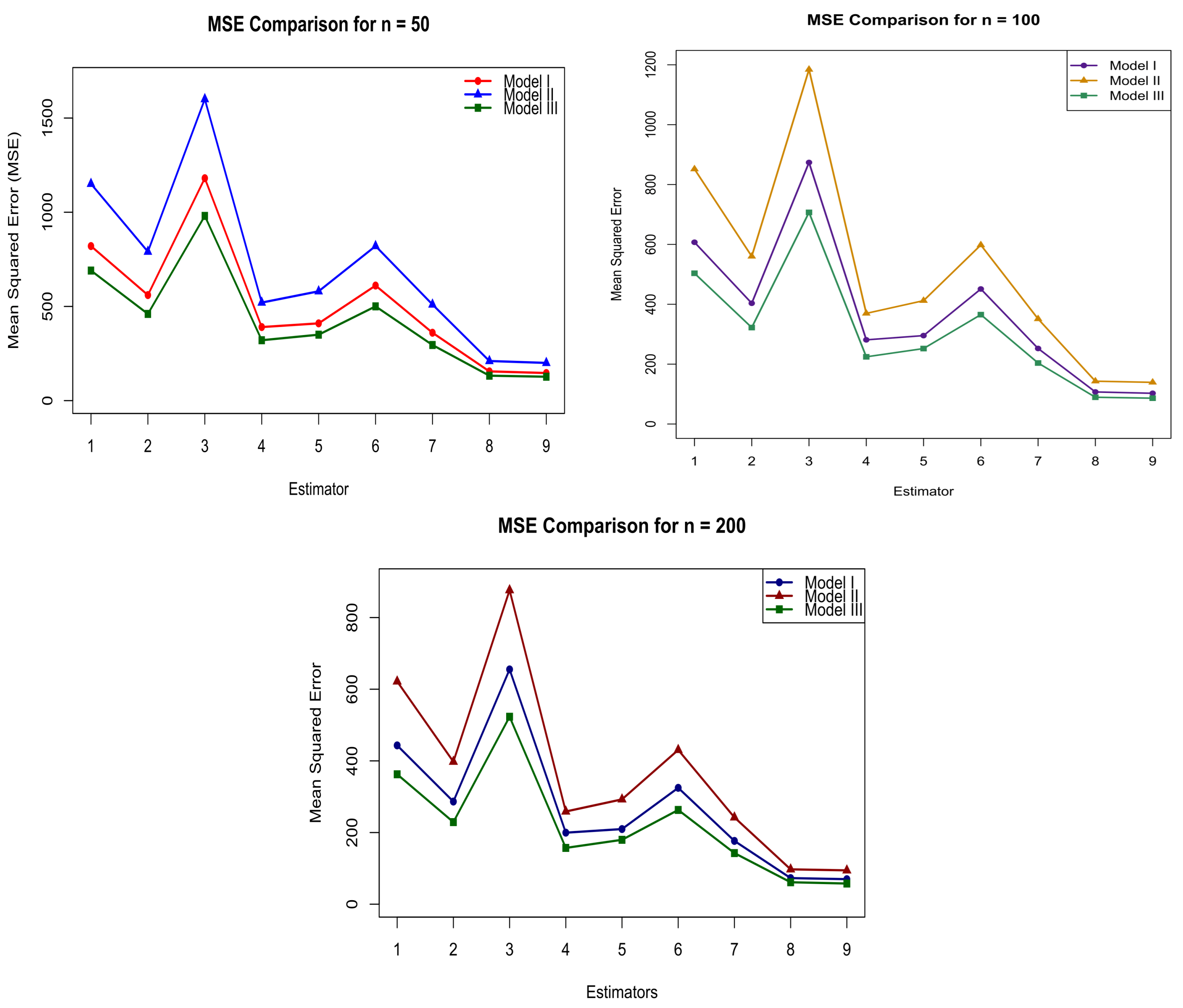
Figure 1 provides a graphical comparison of the MSE values of all competing estimators under different population models and sample sizes. The graphical results are fully consistent with the numerical findings presented in Table 1, Table 2 and Table 3. In all three population models, the proposed estimators show substantially lower MSE values than the classical ratio, product, regression, exponential ratio, exponential product, and generalized exponential estimators. Among the proposed estimators, ${\widehat{\overline{T}}}_{D_{2}sy}$ consistently achieves the lowest MSE, followed by ${\widehat{\overline{T}}}_{D_{1}sy}$, which also demonstrates substantially better efficiency than all existing estimators. Furthermore, the graphical comparison demonstrates that the superiority of the proposed estimators becomes more pronounced as the sample size increases, thereby supporting the theoretical and empirical efficiency of the proposed methodology.

Overall, the simulation study confirms that the proposed class of estimators significantly improves estimation efficiency in systematic sampling. All proposed estimators outperform the existing estimators under linear, nonlinear, and periodic population structures. Among the proposed class, ${\widehat{\overline{T}}}_{D_{2}sy}$ emerges as the most efficient estimator, followed closely by ${\widehat{\overline{T}}}_{D_{1}sy}$. Both proposed estimators consistently outperform all existing estimators considered in this study. Therefore, the proposed estimators provide reliable and efficient alternatives for practical applications in systematic sampling.

6. Empirical Study

To conduct empirical analysis, three independent data sets are used to evaluate and compare the numerical performance of the proposed methodology. The data sets are chosen in order to capture various population structures and variability patterns to enable a thorough and effectively investigated. Based on the comparative analysis, it is necessary to state that the use of multiple data sources makes it strong and not tied to one experimental situation. The entire numerical findings in this paper are obtained on the basis of these three benchmark data sets.

Population 1.

The data set used for empirical evaluation is obtained from Punjab Development Statistics 2014 (pp. 135–136, Tables 89–90) [31], which provides information on government schools for the academic year 2012–2013. The study considers student enrollment as the response variable, while the number of government schools serves as the auxiliary information. Specifically, T denotes the total number of registered students at the primary and middle levels, and V represents the corresponding number of government schools (primary and middle, combined for both boys and girls). These variables are used to assess educational structure and are analyzed to improve estimation efficiency under the proposed systematic sampling framework. The summary statistics are given below:

$$\begin{array}{c}N=72,n=8,k=9,\overline{T}=61319.6500,\overline{V}=638.7222,C_t=0.7715,C_v=0.7971,\hfill \\ S_t=47306.1500,S_v=509.1413,S_{tv}=7127107,{\rho }_t=-0.01023,{\rho }_v=-0.0127,\hfill \\ {\rho }_{tv}=0.29591,D_t=0.9284,D_v=0.9104,D_{tv}=1.0198,F_{tv}=0.2864,\theta =0.1233.\hfill \end{array}$$

Population 2.

The data set used for empirical evaluation is obtained from the 2013 edition of Punjab Development Statistics (p. 226, Table 158) [32] and represents employment and industrial activity across districts for the years 2010 and 2012. In this study, T denotes district-level employment, while V represents the number of registered factories in each district for the corresponding years. These variables are used to examine the association between employment levels and industrial development across districts within a unified analytical framework. The summary statistics are expressed as follows:

$$\begin{array}{c}N=72,n=8,k=9,\overline{T}=25611.4200,\overline{V}=330.9028,C_t=1.6211,C_v=1.3373,\hfill \\ S_t=41518.1400,S_v=442.5282,S_{tv}=13061114,{\rho }_t=0.01433,{\rho }_v=0.01678,\hfill \\ {\rho }_{tv}=0.71089,D_t=1.1003,D_v=1.1175,D_{tv}=0.9846,F_{tv}=0.8617,\theta =0.1233.\hfill \end{array}$$

Population 3.

Represents the medical education sector of Punjab, where each unit corresponds to a district or institution-level observation. The study variable T denotes the number of medical institutions, while the auxiliary variable V represents the number of teaching staff in medical institutes. The auxiliary variable provides information about the human resource capacity of the medical education system and is used to improve the estimation of the study variable. Both variables are obtained from Education-Professional/Medical Institutes (pp. 129–132, Table 86) [31], and are used to improve estimation efficiency under systematic sampling. The summary statistics are defined as follows:

$$\begin{array}{c}N=120,n=10,k=12,\overline{T}=464.1417,\overline{V}=6515.1330,C_t=1.2190,C_v=1.5723,\hfill \\ S_t=565.8045,S_v=10243.4600,S_{tv}=2864838,{\rho }_{tv}=0.49420,{\rho }_t=-0.00381,\hfill \\ {\rho }_v=-0.00700,D_t=0.9657,D_v=0.9361,D_{tv}=1.0316,F_{tv}=0.3832,\theta =0.0992.\hfill \end{array}$$

Three real populations are considered in the empirical study to evaluate the performance of different estimators for the finite population mean under varying population structures. The selected populations represent different patterns of variability, skewness, and association between the study variable and the auxiliary variable. For each population, the mean squared error (MSE) and percentage relative efficiency (PRE) are computed using known population parameters. The systematic sample mean estimator is taken as the benchmark estimator, and its PRE is standardized to 100 for all populations to provide a consistent comparison.

The results presented in

Table 5. MSE and PRE values of various estimators based on real populations.

Estimator	Population 1		Population 2		Population 3
	MSE	PRE	MSE	PRE	MSE	PRE
${\overline{t}}_{sy}$	256,100,038	100.000	233,787,165	100.000	30,658.500	100.000
${\overline{t}}_{Rsy}$	369,139,842	69.378	119,034,561	196.403	41,607.46	73.685
${\overline{t}}_{Psy}$	679,300,643	37.701	671,729,194	34.804	118,581.460	25.854
${\overline{t}}_{lsy}$	233,675,459	109.597	115,639,984	202.168	23,167.760	132.332
${\overline{t}}_{Resy}$	237,960,364	107.623	150,539,199	155.290	22,460.750	136.498
${\overline{t}}_{Pesy}$	408,299,814	62.724	397,832,488	58.765	63,574.240	48.225
${\overline{t}}_{aesy}$	229,045,448	111.812	139,177,060	167.978	22,110.480	138.661
${\widehat{\overline{T}}}_{D_{1}sy}$	64,513,653	396.970	37,218,357	628.150	12,161.680	252.091
${\widehat{\overline{T}}}_{D_{2}sy}$	64,203,246	398.880	37,033,309	631.280	11,965.85	256.217

indicate that the proposed estimators provide substantial improvements over the traditional ratio, product, regression, and exponential-type estimators. The conventional estimators show unstable performance because their efficiency depends mainly on linear relationships and may deteriorate when the auxiliary variable contains large variation or extreme observations. In contrast, the proposed estimators utilize transformed auxiliary information, allowing them to better accommodate nonlinear relationships and heterogeneous population structures.

For Population 1, where the auxiliary variable exhibits considerable variability and the study variable shows substantial fluctuations, the estimator ${\widehat{\overline{T}}}_{D_{2}sy}$ provides the best performance. The geometric-adjusted estimator achieves the smallest MSE and the highest PRE among all competing estimators, indicating that the geometric transformation effectively utilizes the available auxiliary information and provides a stable estimation framework for this population. For Population 2, where the relationship between the study and auxiliary variables is comparatively stronger, the estimator ${\widehat{\overline{T}}}_{D_{2}sy}$ emerges as the most efficient estimator. The geometric adjustment effectively utilizes the auxiliary information and produces the lowest MSE and highest PRE, demonstrating its suitability for this population structure. For Population 3, the estimator ${\widehat{\overline{T}}}_{D_{2}sy}$ again achieves the highest efficiency among all competing estimators. Its superior performance indicates that the geometric transformation provides a more effective adjustment under this population structure, resulting in a noticeable reduction in MSE and a corresponding increase in PRE.

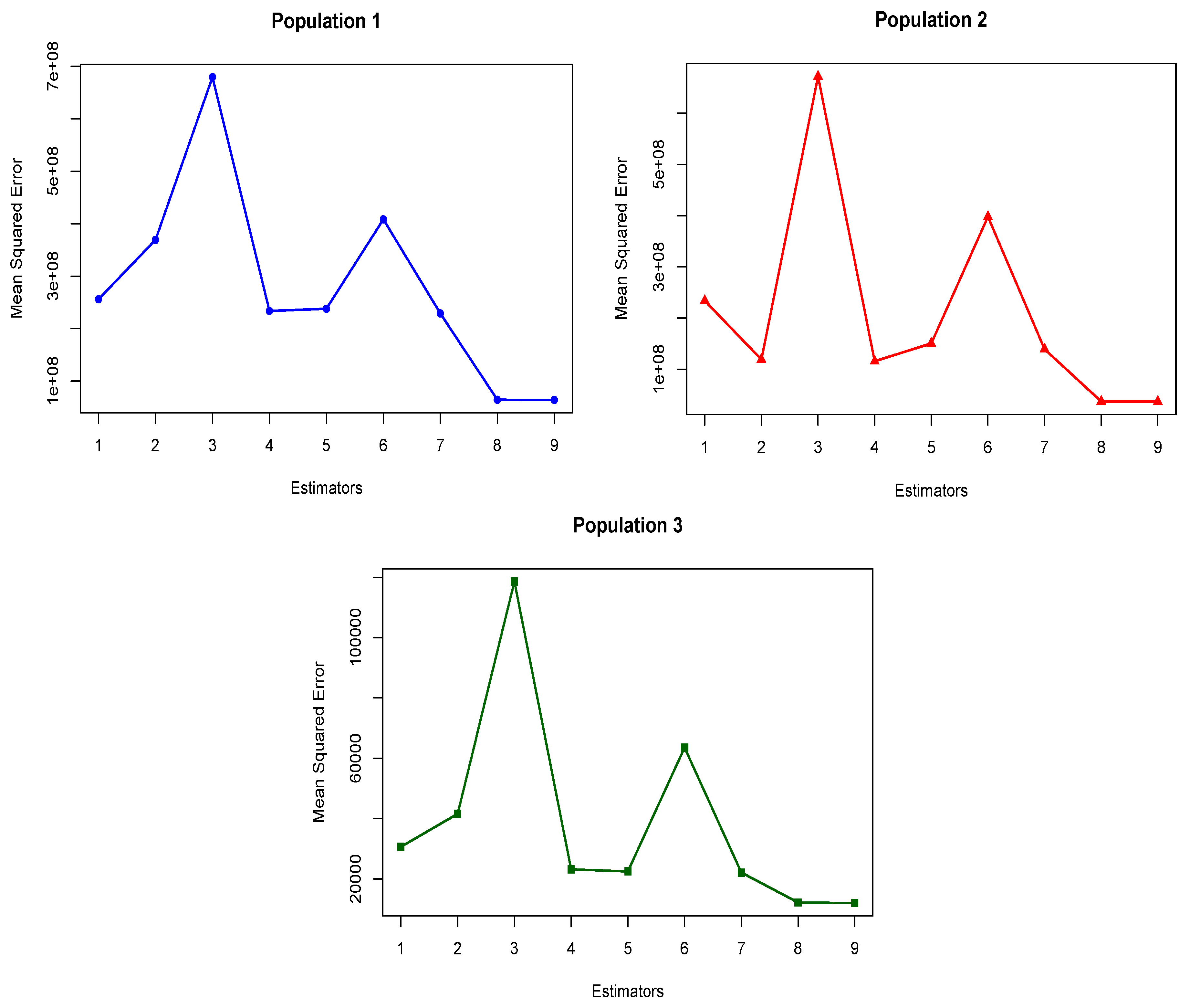
Figure 2 presents the graphical comparison of estimator performance for the three real populations. The graphical results support the findings reported in Table 5, where the proposed estimators generally achieve smaller MSE values than existing methods. The results demonstrate that no single proposed estimator dominates for every population; rather, the most efficient estimator depends on the distributional characteristics of the auxiliary variable and its relationship with the study variable. The improved efficiency of the proposed estimators is mainly attributed to their effective use of auxiliary information through nonlinear transformations. The harmonic component in ${\widehat{\overline{T}}}_{D_{1}sy}$ provides stability against extreme observations and is suitable for populations with high variability. The geometric component in ${\widehat{\overline{T}}}_{D_{2}sy}$ performs better when the study and auxiliary variables follow a multiplicative pattern or contain strong positive association.

Overall, the empirical findings confirm the theoretical development and show that the proposed estimators provide efficient alternatives for estimating the finite population mean under systematic sampling. The results highlight that transformation-based estimators can successfully exploit auxiliary information and achieve better performance than traditional estimators under diverse real-life population structures.

7. Limitations of the Study

Despite the encouraging theoretical and empirical findings, the present study has certain limitations. The proposed estimators are developed under first-order approximation assumptions, and their performance may vary under highly irregular population structures or weak auxiliary relationships. In addition, the simulation study is based on artificially generated populations and a limited number of real data sets. Therefore, further investigation using more diverse real-world populations and alternative sampling environments can be valuable to fully assess the practical stability and overall applicability of the proposed estimators.

8. Conclusions and Future Research Directions

This paper proposed a novel class of weighted hybrid estimators for estimating the finite population mean under systematic sampling by using harmonic and geometric transformations of auxiliary information. The proposed estimators were developed to overcome the limitations of classical linear, ratio, product, regression, and exponential-type estimators, particularly under nonlinear relationships, skewness, and periodic population structures.

First-order Taylor series approximations were used to derive the bias and mean squared error (MSE) expressions of the proposed estimators, and the optimal weights were obtained by minimizing the MSE. The performance of the proposed estimators was evaluated through extensive simulation studies under three different population models, namely linear, nonlinear, and periodic, for sample sizes $n=50,100,200$, as well as through real-life applications involving three real populations.

The simulation results showed that the proposed estimators consistently outperformed all classical estimators across all considered scenarios. Among the proposed class, the estimator ${\widehat{\overline{T}}}_{D_{2}sy}$ consistently achieved the smallest MSE and the highest percentage relative efficiency (PRE) across all population models and sample sizes. The estimator ${\widehat{\overline{T}}}_{D_{1}sy}$ also demonstrated substantial improvement over the traditional estimators and remained highly competitive. The results further confirmed that the MSE decreased as the sample size increased from $n=50$ to $n=200$, indicating improved estimation accuracy and stability across different population structures. The empirical study based on three real populations further confirmed the effectiveness of the proposed estimators. Among all estimators considered, ${\widehat{\overline{T}}}_{D_{2}sy}$ consistently achieved the lowest MSE and the highest PRE across all three populations, demonstrating its superior performance. The estimator ${\widehat{\overline{T}}}_{D_{1}sy}$ also performed remarkably well, consistently after ${\widehat{\overline{T}}}_{D_{2}sy}$ in terms of efficiency. These findings demonstrate the practical applicability and robustness of the proposed methodology under diverse real population structures. In conclusion, the proposed class of estimators provides efficient and reliable alternatives for estimating the finite population mean under systematic sampling. Overall, ${\widehat{\overline{T}}}_{D_{2}sy}$ emerged as the most efficient estimator in both the simulation and empirical studies, consistently exhibiting the lowest MSE and the highest PRE among all the estimators considered. Therefore, the proposed estimators are recommended for practical applications when suitable auxiliary information is available.

In summary, all three proposed estimators provide efficient alternatives for estimating the finite population mean under systematic sampling. The results demonstrate that the proposed estimators substantially improve estimation efficiency by effectively utilizing auxiliary information. Among the proposed estimators, ${\widehat{\overline{T}}}_{D_{2}sy}$ consistently shows the best performance across both the simulation study and all three real populations, achieving the lowest MSE and the highest PRE. Although ${\widehat{\overline{T}}}_{D_{1}sy}$ also performs competitively and generally ranks second, ${\widehat{\overline{T}}}_{D_{2}sy}$ provides the most reliable and efficient estimator for the populations considered. These findings highlight the practical applicability of the proposed estimators in survey sampling under diverse population structures. Although the present study evaluates the theoretical optimal performance of the proposed estimators under known population quantities, future research will focus on developing feasible plug-in implementations based entirely on sample-derived estimates and investigating their theoretical and empirical properties. The proposed estimators also offer several opportunities for future research and practical applications. In real-life survey environments, the suggested methodology can be applied in agricultural production surveys, environmental monitoring studies, public health investigations, industrial quality control, and economic and labor force surveys where systematic sampling is commonly used and auxiliary information is available. Future studies may further extend the proposed framework to situations involving multiple auxiliary variables, non-response, missing observations, and measurement errors. In addition, using machine-learning-based auxiliary predictors and adaptive systematic sampling strategies may further improve estimation efficiency in complex population structures.

References

1. Cochran, W.G. Relative efficiency of systematic and stratified random samples for a certain class of population. Ann. Math. Stat. 1946, 17, 164–177. [Google Scholar] [CrossRef]
2. Cochran, W.G. Sampling Techniques, 3rd ed.; John Wiley and Sons: Hoboken, NJ, USA, 1977. [Google Scholar]
3. Kish, L. Survey Sampling; John Wiley & Sons: New York, NY, USA, 1965. [Google Scholar]
4. Yates, F. Systematic sampling. Philos. Trans. R. Soc. A 1948, 241, 345–377. [Google Scholar] [CrossRef]
5. Gautschi, W. Some remarks on systematic sampling. Ann. Math. Stat. 1957, 28, 385–394. [Google Scholar] [CrossRef]
6. Hajeck, J. Optimum strategy and other problems in probability sampling. Čas. Pěst. Mat. 1959, 84, 387–423. [Google Scholar] [CrossRef]
7. Madow, W.G. On the theory of systematic sampling. Ann. Math. Stat. 1948, 19, 333–354. [Google Scholar]
8. Hansen, M.H.; Hurwitz, W.N. On the theory of sampling from finite populations. Ann. Math. Stat. 1943, 14, 333–362. [Google Scholar] [CrossRef]
9. Lahiri, D.B. On the question of bias of systematic sampling. Proc. World Pet. Congr. 1954, 6, 349–362. [Google Scholar] [CrossRef]
10. Swain, A.K.P.C. The use of systematic sampling in ratio estimate. J. Indian Stat. Assoc. 1964, 2, 160–164. [Google Scholar]
11. Murthy, M.N. Sampling Theory and Methods, 2nd ed.; Statistics and Public Policy: Calcutta, India, 1967.
12. Shukla, N.D. Systematic sampling and product method of estimation. In Proceedings of the All-India Seminar on Demography and Statistics; BHU: Varanasi, India, 1971. [Google Scholar]
13. Kushwaha, K.S.; Singh, H.P. Class of almost unbiased ratio and product estimators in systematic sampling. J. Indian Soc. Agric. Stat. 1989, 41, 193–205. [Google Scholar]
14. Kushwaha, S.N.S.; Kushwaha, K.S. A class of ratio, product and difference (RPD) estimators in systematic sampling. Microelectron. Reliab. 1993, 33, 455–457. [Google Scholar] [CrossRef]
15. Singh, R.; Singh, H.P. Almost unbiased ratio and product-type estimators in systematic sampling. Qüestiió Quadr. Estad. Investig. Oper. 1998, 22, 403–416. [Google Scholar]
16. Singh, H.P.; Tailor, R.; Jatwa, N.K. Modified ratio and product estimators for population mean in systematic sampling. J. Mod. Appl. Stat. Methods 2011, 10, 424–435. [Google Scholar] [CrossRef]
17. Singh, H.P.; Solanki, R.S. An efficient class of estimators for the population mean using auxiliary information in systematic sampling. J. Stat. Theory Pract. 2012, 6, 274–285. [Google Scholar] [CrossRef]
18. Singh, H.P.; Jatwa, N.K. A class of exponential type estimators in systematic sampling. Econ. Qual. Control 2013, 27, 195–208. [Google Scholar] [CrossRef]
19. Tailor, T.; Jatwa, N.K.; Singh, H.P. A ratio-cum-product estimator of finite population mean in systematic sampling. Stat. Transit. 2013, 14, 391–398. [Google Scholar] [CrossRef]
20. Khan, M.; Singh, R. Estimation of population mean in chain ratio-type estimator under systematic sampling. J. Probab. Stat. 2015, 2015, 248374. [Google Scholar] [CrossRef]
21. Noor-ul-Amin, M.; Javaid, A.; Hanif, M. Estimation of population mean in systematic random sampling using auxiliary information. J. Stat. Manag. Syst. 2017, 20, 1095–1106. [Google Scholar] [CrossRef]
22. Javaid, A.; Noor-ul-Amin, M.; Hanif, M. Modified ratio estimator in systematic random sampling under non-response. Proc. Natl. Acad. Sci. India Sect. A Phys. Sci. 2019, 89, 817–825. [Google Scholar] [CrossRef]
23. Khan, M.; Shabbir, J. Some improved ratio, product, and regression estimators of finite population mean using minimum and maximum values. Sci. World J. 2013, 2013, 431868. [Google Scholar] [CrossRef] [PubMed]
24. Qureshi, M.N.; Khalil, S.; Hanif, M. Generalized semi exponential type estimator under systematic sampling. J. Stat. Theory Appl. 2018, 17, 283–290. [Google Scholar] [CrossRef]
25. Iftikhar, A.; Shi, H.; Hussain, S.; Qayyum, A.; El-Morshedy, M.; Al-Marzouki, S. Estimation of finite population mean in presence of maximum and minimum values under systematic sampling scheme. AIMS Math. 2022, 7, 9825–9834. [Google Scholar] [CrossRef]
26. El-Morshedy, M.; Hussain, S.; Ullah, K.; Khalil, A.; Shabbir, J.; Mansoor, W. Finite population mean estimation under systematic sampling scheme in presence of maximum and minimum values using two auxiliary variables. Math. Probl. Eng. 2022, 2022, 2703178. [Google Scholar] [CrossRef]
27. Koçyiğit, E.G. New memory-type estimators for systematic sampling. J. Adv. Res. Nat. Appl. Sci. 2025, 11, 224–236. [Google Scholar] [CrossRef]
28. Karim, A.; Khan, H.; Mahmood, Y.; Riaz, M.; Ahmad, S. On estimation and monitoring of population mean using systematic sampling under an exponentially weighted moving average scheme. Pak. J. Stat. Oper. Res. 2024, 20, 517–531. [Google Scholar] [CrossRef]
29. Pal, S.K.; Mahmud, S.A.; Singh, H.P. An efficient estimation of finite population mean through difference estimator in systematic sampling. Afr. Mat. 2025, 36, 14. [Google Scholar] [CrossRef]
30. Nagy, M.; Qureshi, M.N.; Shaheen, N.; Hanif, M. Mean estimation using memory-type estimators in systematic sampling for time-scaled surveys. Mathematics 2026, 14, 1180. [Google Scholar] [CrossRef]
31. Bureau of Statistics. Punjab Development Statistics Government of the Punjab, Lahore, Pakistan; Bureau of Statistics: Islamabad, Pakistan, 2014.
32. Bureau of Statistics. Punjab Development Statistics Government of the Punjab, Lahore, Pakistan; Bureau of Statistics: Islamabad, Pakistan, 2013.
Figure 1. Graphical representation of the simulation results obtained under different population models. Estimators 1–7 represent the existing estimators, whereas estimators 8–9 denote the proposed estimators.
Axioms 15 00590 g001
Figure 2. Graphical representation of the results obtained under different real populations. Estimators 1–7 represent the existing estimators, whereas estimators 8–9 denote the proposed estimators.
Axioms 15 00590 g002