Acceptance Sampling Plans for Exponential- and Weibull-Distributed Lifetimes Under the Group Sampling Framework

Abstract

Product lifetime is a critical quality characteristic of electronic products. Among various lifetime models, the Weibull distribution is one of the most flexible and widely used distributions in reliability analysis because it can describe different failure rate patterns through its shape parameter. In this study, the Weibull distribution is treated as the primary lifetime model, while the exponential distribution is included as a simpler benchmark model and as a special case of the Weibull distribution with shape parameter m = 1. Based on the lifetime performance index, this research applies the group sampling concept to design two lifetime acceptance sampling plans under these lifetime distributions. The optimal sampling plan parameters of the lifetime acceptance sampling plans are determined by minimizing the number of groups while satisfying the two-point principle of the operating characteristic curve. For practical purposes, the parameters of the proposed plan are tabulated for some combinations of quality levels with commonly used producer risk and consumer risk. Moreover, a comparative analysis of the two lifetime testing methods is presented, and the results show that Testing Method II proposed in this study can implement sampling inspection more efficiently. Finally, an example is used to illustrate the proposed methodology.

1. Introduction

To ensure the outgoing quality of products, buyers or suppliers typically would conduct acceptance sampling on critical quality characteristics. Acceptance sampling is a statistical tool used to make decisions regarding whether the product lot should be released for consumer use or not [1]. Based on the inspection results, a decision is made as to whether the lot should be accepted. This procedure constitutes what is known as an acceptance sampling plan. In quality control, acceptance sampling plays a pivotal role and is widely applied across various stages, including the inspection of raw materials, semi-products, final products, and pre-shipments. A well-designed sampling plan can effectively reduce the difference between the actual supply quantity and order quantity [2].

The following outlines some recent important studies on acceptance sampling. Wu et al. [3] designed acceptance sampling plans based on the lifetime performance index for an exponential population with and without censoring using statistical and decision-theoretic methodologies that minimize the number of failures required during inspection. Saleh et al. [4] reviewed some important literature on the use of the repetitive sampling technique with quality control charts. They raised some important concerns and questions regarding its application and underlying assumptions. They showed that a fixed sample size method that requires on average the same amount of sampling can be designed to have as good or better statistical properties when monitoring with data that are normally distributed. Repetitive sampling methods can be useful, however, when monitoring with count data. Lee et al. [5] designed an SSP and an RGSP specifically for exponential lifetime products. In particular, their study utilized the progressively Type II right-censored sample as the data type for lifetime testing. Banihashemi et al. [6] proposed a hybrid sampling plan that combines prior information and finite repetition sampling based on the functional $C_{pk}$ for circular profiles. Their method incorporates a flexible resampling policy by integrating past information, enabling adjustable evaluation of different quality. Wang and Wu [7] introduced an adaptive VQSS (AVQSS) model that builds on traditional VQSS by simultaneously adjusting both the required number of failures and acceptance criteria to construct normal and tightened inspections. By integrating AVQSS with the lifetime performance index, they provided a more robust framework for quantifying and evaluating product reliability. Wu et al. [8] introduced single and double sampling plans to be within the framework of time-truncated life testing, and the percentile life was used as a measure of reliability. They derived operating characteristic functions for both single and double sampling plans and established optimization models to minimize the required sample size for testing, simultaneously accounting for Type I and Type II errors. They also presented an algorithm for solving these optimization models and conducted an in-depth analysis of the proposed methods, outlining their respective strengths and limitations for real-world applications. Wang et al. [9] proposed the failure-censored tightened-normal-tightened sampling system (FTSS), which utilizes the lifetime performance index to enable adaptive decision-making. A comparative analysis demonstrated that the proposed FTSS enhances cost-effectiveness and discriminatory power in reliability assessment, making it particularly beneficial for high-cost lifetime testing. It is worth noting that the aforementioned papers frequently utilize the concept of process capability indices (PCIs). For more information on the concept of PCIs, please refer to [10,11,12,13,14].

When the key quality characteristic of a product is lifetime, acceptance sampling becomes particularly critical. From the above important recent literature, we can see that many acceptance sampling plans are designed specifically for product lifetime. Product lifetime is one of the most fundamental indicators of quality: a longer lifetime reflects higher reliability, which in turn enhances consumer confidence and market competitiveness. Reliability, in essence, represents the probability that a product or system performs its intended function without failure for a specified period under stated conditions. In reliability analysis, product lifetimes may be modeled by several probability distributions depending on the underlying failure mechanism. Commonly used lifetime distributions include the Weibull, lognormal, gamma, log-gamma, two-parameter Birnbaum–Saunders, Lindley, generalized exponential, and generalized Pareto distributions. Among these, the Weibull distribution is particularly flexible because it can describe decreasing, constant, and increasing failure rate patterns through its shape parameter. When the Weibull shape parameter is equal to 1, the Weibull distribution reduces to the exponential distribution, which corresponds to a constant failure rate. For critical electronic components, ensuring high reliability is paramount. A failure in these components may trigger severe system-level consequences. For instance, defects in the key parts of a power generation control system or aircraft engine could lead to catastrophic operational interruptions and even pose significant threats to human safety. Therefore, establishing an effective lifetime acceptance sampling plan is of strategic importance for safeguarding product reliability.

Before deciding on lot acceptance, it is common to subject the product to a lifetime testing plan to ensure that a production lot meets the required lifetime performance. However, lifetime testing is inherently destructive, making 100% inspection infeasible for either producers or consumers. Only a subset of the lot can be sampled for evaluation. Moreover, due to advancements in modern technology, contemporary electronic components often exhibit prolonged lifetimes, rendering full-duration lifetime tests prohibitively time- and cost-intensive. Consequently, to balance quality assurance with operational efficiency, two commonly used truncation schemes, time-truncated tests and failure-truncated tests, are often adopted in lifetime testing. In time-terminated tests (Type I censoring), the experiment is terminated after a pre-specified test time; in failure-terminated tests (Type II censoring), the experiment stops once a predetermined number of failures occur.

In practical manufacturing and inspection settings, multiple test devices are commonly used, with each device being able to assess numerous items simultaneously. A testing unit containing multiple items is referred to as a group, and the number of test items within each group is called the group sample size. Acceptance sampling plans designed under this group-based framework are known as group acceptance sampling plans (GASPs). Compared to conventional acceptance sampling plans, GASPs offer substantial savings in testing time and cost by leveraging parallel testing across multiple groups. Specifically, for failure-terminated lifetime tests (Type II censoring), adopting group testing allows the required number of failures to be reached more rapidly, thereby significantly reducing overall testing duration. Moreover, group testing yields more information for evaluating lifetime performance, enhancing the statistical power of the plan.

Due to the economic benefits of group sampling, some studies have explored the integration of group sampling into lifetime acceptance plans. Jun et al. [15] considered lifetime data following a Weibull distribution, setting the first failure within each group as the termination criterion. Their study constructed both single and double lifetime acceptance sampling plans with the minimum number of groups. Aslam and Jun [16] and Aslam et al. [17] considered the lifetimes of products following the Weibull and gamma distributions, respectively. With the quality metric defined as the ratio of the observed mean life to a target mean life, they designed single acceptance sampling plans for life testing that a lot is accepted only when the number of failed items in every group is below a pre-specified threshold. Rao [18] considered the lifetime of products following a generalized exponential distribution. Aslam et al. [19] proposed an improved group life sampling plan, considering that the product lifetime follows a Weibull distribution. In their study, the acceptance of the lot must meet the requirement that the number of failed products in at least k groups must be less than a certain number. Their study found that compared to previous lot acceptance criteria, this lot acceptance criterion can reduce the sample size of inspections. For more literature about lifetime acceptance plans designed with group sampling, readers can see [20,21].

To the best of our knowledge, although various group acceptance sampling plans (GASPs) have been widely investigated in the literature, they predominantly rely on mean lifetimes or percentiles as their primary quality metrics. No prior research has integrated the group sampling framework with the lifetime performance index, $C_L$, under a failure-terminated (Type II censoring) scheme. The index $C_L$ possesses superior practical merit because it directly relates process capability to the lower specification limit required by consumers, providing a more reliable quality assurance tool for modern manufacturing. In view of the above, the development of an effective lifetime acceptance sampling plan is both necessary and of significant practical importance. Lifetime testing inherently involves substantial time and cost; however, when permissible, integrating group sampling techniques into lifetime testing offers the potential to greatly enhance testing efficiency and reduce resource expenditure. To provide the maximum flexibility for practitioners, this paper proposes two distinct testing methods. Testing Method I terminates upon the first failure in each group, offering an exceptionally rapid inspection duration that is ideal when testing time is strictly constrained. Conversely, Testing Method II requires fewer test groups and smaller total sample sizes, providing a highly cost-effective alternative when multi-channel testing equipment is limited or expensive. The proposed methodology not only addresses the high cost and lengthy duration typically associated with lifetime testing but also provides a systematic and statistically rigorous framework that can serve as a practical reference for industrial implementation. The remainder of this paper is organized as follows. Section 2 offers a brief overview of lifetime performance index $C_L$. Section 3 presents the design of the proposed lifetime testing plan. Section 4 displays the parameter tables of the proposed methodology. Section 5 provides a comparative analysis of the two lifetime testing plans. An illustrative example is presented in Section 6. Finally, conclusions are drawn in Section 7.

2. Lifetime Performance Index

Product lifetime is a larger-the-better quality characteristic; longer lifetimes indicate higher quality and reliability. Typically, a product must exceed a minimum lifetime threshold to meet customer satisfaction and reliability requirements. Montgomery [22] introduced the lifetime performance index $C_L$ as a measure for assessing electronic component reliability. Many studies use the lifetime performance index as an evaluation of product lifetime. When a product is required to meet a specified minimum lifetime threshold L, the index $C_L$ is defined as

$$C_L={\displaystyle \frac{{\mu }_T-L}{{\sigma }_T}},$$

(1)

where ${\mu }_T$ and ${\sigma }_T$ are the population mean and standard deviation of product lifetime, and L denotes the lower specification limit.

Tong et al. [23] constructed a uniformly minimum variance unbiased (UMVU) estimator of $C_L$ under an exponential distribution. The UMVU estimator of $C_L$ was then utilized to develop a hypothesis testing procedure. Purchasers can employ the testing procedure to determine whether the lifetime of electronic components adheres to the required level. Manufacturers can also utilize this procedure to enhance process capability. Alsaedi et al. [24] developed a maximum likelihood estimator (MLE) for $C_L$ for the parameter of a mixture Rayleigh Half-Normal (RHN) distribution under progressively Type II right-censored samples under the constraint of knowing the lower specification limit L. Additionally, they suggested an asymptotic normal distribution for the MLE for $C_L$ in order to construct a mechanism for evaluating products’ lifespan efficiency. Wu and Lu [25] proposed the MLE to estimate $C_L$ based on the progressive Type I interval-censored sample when the lifetime of products possesses a one-parameter Pareto distribution. The asymptotic distribution of this estimator was also investigated. Based on the testing procedure for the lifetime of products following the Chen distribution, Wu and Song [26] determined an experimental design for progressive Type I interval censoring to achieve the desired power level while minimizing total experimental cost.

As mentioned in the above section, there are significant differences between Type I censoring and Type II censoring. In a time-terminated test (Type I censoring), a fixed sample of products is subjected to testing, and the test is terminated once a pre-specified time limit is reached. The decision to accept or reject a given lot is based on the cumulative number of failures observed at the termination time. Let n denote the sample size and t₀ the predetermined test duration. Let t₁, t₂, …, t_a represent the failure times of the first through the a-th failed units by time t₀. The estimate of the average lifetime is calculated accordingly.

$$\widehat{\theta }=\left[{\displaystyle \sum _{i=1}^a{t}_i+(n-a)t_0}\right]/a.$$

(2)

The lot acceptance criterion is as follows: if the number of observed failures a does not exceed the acceptance number c, the lot is accepted; otherwise, it is rejected.

In a failure-terminated test (Type II censoring), a subset of units is placed under test, and the experiment is terminated once a predetermined number of product failures has occurred. Lot acceptance is determined based on the cumulative lifetime data of the failed units at the termination point. Let n denote the sample size and r the predetermined number of failures, and let t₁, t₂, …, t_r represent the ordered failure times of the first through the r-th failed units, respectively. The estimator of the mean product lifetime is then expressed as

$$\widehat{\theta }=\left[{\displaystyle \sum _{i=1}^r{t}_i+(n-r)t_r}\right]/r.$$

(3)

The lot acceptance rule is as follows: if the estimated mean lifetime $\widehat{\theta }$ exceeds the acceptance threshold c, the lot is accepted; otherwise, the lot is rejected. For standardized procedures related to reliability and life testing, reference may be made to the Quality Control and Reliability Handbook H-108, developed by the U.S. Department of Defense in 1960.

In this paper, we adopt the failure-terminated (Type II censoring) lifetime testing approach as the experimental framework and incorporate a group acceptance sampling methodology to employ $C_L$ as the core quality metric for evaluating product lifetime.

2.1. Lifetime Following an Exponential Distribution

When the product lifetime T follows an exponential distribution, then

$$f(T)=\lambda e^{-\lambda T}, T\ge 0,$$

(4)

where $\lambda$ > 0 is the rate parameter. Since the mean and variance of T are ${\mu }_T = 1/\lambda$ and ${\sigma }_T^2 = {1/\lambda }^2$, the lifetime performance index $C_L$ can be expressed as

$$C_L={\displaystyle \frac{1/\lambda -L}{1/\lambda }}=1-\lambda L,$$

(5)

and the reliability R and defect rate p can be expressed as follows, respectively:

$$R=P(T\ge L)=e^{-\lambda L}=e^{C_L-1},$$

(6)

$$p=P(T<L)=1-e^{-\lambda L}=1-e^{C_L-1}.$$

(7)

2.2. Lifetime Following a Weibull Distribution

When the product lifetime T follows a Weibull distribution, then

$$f(T)=\lambda m{\left(\lambda T\right)}^{m-1}{e}^{-{\left(\lambda T\right)}^m}, T\ge 0,$$

(8)

where m > 0 is the shape parameter. Since the mean and variance of T are ${\mu }_T = (1/\lambda \left)\mathsf{\Gamma }\right(1+1/m)$ and ${\sigma }_T^2 = (1/{\lambda }^2)\left[\mathsf{\Gamma }\left(1+2/m\right)-{\mathsf{\Gamma }}^2\left(1+1/m\right)\right]$, the lifetime performance index $C_L$ can be expressed as

$$C_L={\displaystyle \frac{\frac{1}{\lambda }\mathsf{\Gamma }\left(1+\frac{1}{m}\right)-L}{\sqrt{\frac{1}{{\lambda }^2}\left[\mathsf{\Gamma }\left(1+\frac{2}{m}\right)-{\mathsf{\Gamma }}^2\left(1+\frac{1}{m}\right)\right]}}}={\displaystyle \frac{\mathsf{\Gamma }\left(1+\frac{1}{m}\right)-\lambda L}{k}},$$

(9)

where k = $\sqrt{(1/{\lambda }^2\left)\right[\mathsf{\Gamma }\left(1+2/m\right)-{\mathsf{\Gamma }}^2\left(1+1/m\right)]}$, and the reliability and defect rate can be formulated as the following Equations (10) and (11), respectively:

$$R=P(T\ge L)=e^{-{\left(\lambda L\right)}^m}=e^{{\left(k{C}_L-\mathsf{\Gamma }\left(1+{\displaystyle \frac{1}{m}}\right)\right)}^m},$$

(10)

$$p=P(T<L)=1-e^{-{\left(\lambda L\right)}^m}=1-e^{{\left(k{C}_L-\mathsf{\Gamma }\left(1+{\displaystyle \frac{1}{m}}\right)\right)}^m}\hspace{0.33em}.$$

(11)

3. The Design of the Proposed Methodology

This study integrates the concept of Type II censoring with a group sampling framework to design two alternative lifetime testing schemes for product evaluation. The sampling plans are described as follows.

3.1. Designing Lifetime Testing Plans Using Group Sampling

• Testing Method I

The experimental procedure is presented as follows:

(1)

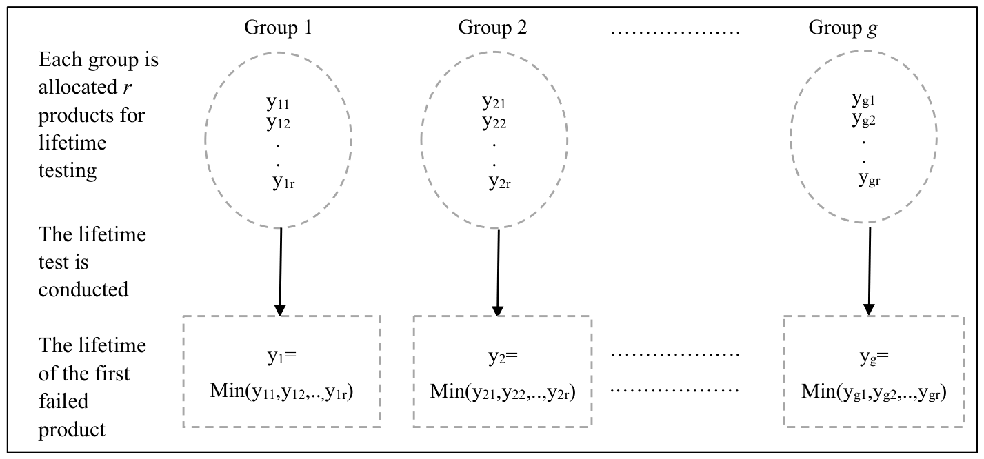
Partition the sample into g groups and randomly select n test units (n ≥ g), allocating r units to each group, n = gr.

(2)

Conduct lifetime tests simultaneously on all groups. For each group, terminate the test immediately once the first failure occurs.

(3)

Compute the estimated lifetime performance index based on the first failure data from all g groups.

(4)

Accept the lot if $C_L$ exceeds the pre-specified acceptance threshold; otherwise, reject the lot.

A schematic representation of Testing Method I is provided in Figure 1.

B.

Testing Method II

The experimental procedure is presented as follows:

(1)

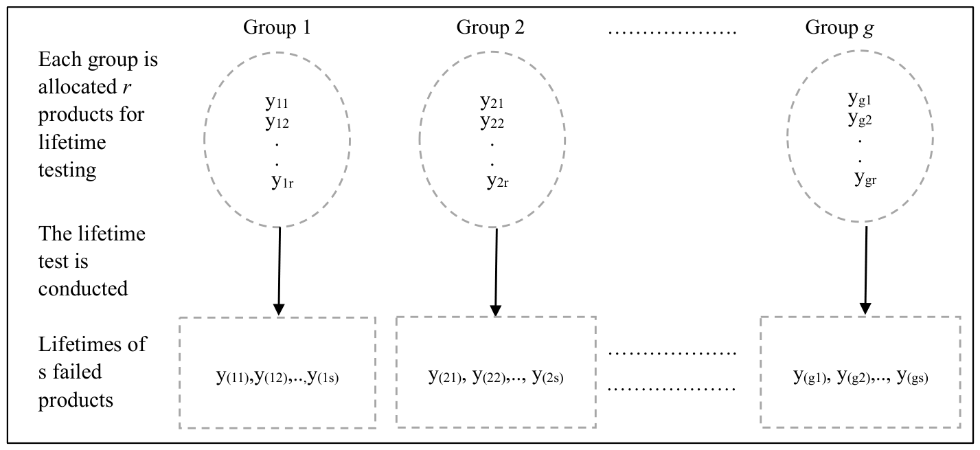
Partition the sample into g groups and randomly select n test units (n ≥ g), allocating r units to each group, n = gr.

(2)

Conduct lifetime tests simultaneously on all groups. For each group, terminate testing when the s-th failure occurs.

(3)

Estimate the lifetime performance index for each group using the s failure data.

(4)

Accept the lot if at least v of the g groups yield $C_L$ values exceeding the acceptance threshold; otherwise, reject the lot.

A schematic representation of Testing Method II is provided in Figure 2.

3.2. Estimation of Lifetime Performance Index and Lot Acceptance Probability

• Testing Method I

(1)

Lifetime Following an Exponential Distribution

Based on Equation (5), the point estimator $\widehat{C_L^{\prime }}$ of $C_L^{\prime }$ is expressed as

$$\widehat{C_L^{\prime }}=1-\widehat{\lambda }L.$$

(12)

Using the MLE method to obtain $\widehat{\lambda }$, and subsequently invoking the invariance property of the MLE, the estimator of $\widehat{C_L^{\prime }}$ can be derived. Let y_i denote the first failure lifetime in group i, with $P(y_i>T) = P(y_{i1}>T,\hspace{0.33em}{y}_{i2}>T, \dots ,y_{\mathrm{ir}}>T) = e^{-r\lambda T}$, i = 1, 2, …, g, where y_i1, y_i2, …, y_ir is the lifetime of the r-th unit in group i. Since y_i follows an exponential distribution with parameter $r\lambda$, the likelihood function can be constructed accordingly $f(y_1, y_2, \dots ,y_g) =$${(\lambda r)}^g{e}^{-\lambda r{\displaystyle {\sum }_{i=1}^g{y}_i}}$. By applying the differentiation method, the MLE of $\widehat{\lambda }$ can be obtained as $g/r{\displaystyle {\sum }_{i=1}^g{y}_i}$, and subsequently the MLE of $\widehat{C_L^{\prime }}$ can be expressed as $\widehat{C_L^{\prime }}=1-(g/r{\displaystyle {\sum }_{i=1}^g{y}_i})L$. Given that the distribution of ${\sum }_{i=1}^g{y}_i$ follows a gamma distribution with parameters (g, $r\lambda$), we can obtain that

$$E\left(\widehat{C_L^{\prime }}\right)=E\left(1-{\displaystyle \frac{g}{r{\displaystyle \sum _{i=1}^g{y}_i}}}L\right)=1-{\displaystyle \frac{gL}{r}}E\left({\displaystyle \frac{1}{{\displaystyle \sum _{i=1}^g{y}_i}}}\right)=1-{\displaystyle \frac{gL}{r}}{\displaystyle \frac{r\lambda }{g-1}}=1-{\displaystyle \frac{g}{g-1}}\lambda L.$$

(13)

Accordingly, the unbiased estimator can be defined as

$${\widehat{C}}_L=1-{\displaystyle \frac{g-1}{r{\displaystyle \sum _{i=1}^g{y}_i}}}L.$$

(14)

Based on Equation (14), the lot acceptance probability using ${\widehat{C}}_L$ as the decision criterion can be derived as follows:

$$P(C_L)=P({\widehat{C}}_L>c)=P\left(1-{\displaystyle \frac{g-1}{r{\displaystyle \sum _{i=1}^g{y}_i}}}L>c\right),$$

$$=P\left(r{\displaystyle \sum _{i=1}^g{y}_i}>{\displaystyle \frac{(g-1)}{1-c}}L\hspace{0.33em}\right)=P\left(2\lambda r{\displaystyle \sum _{i=1}^g{y}_i}>{\displaystyle \frac{2\lambda (g-1)}{1-c}}L\hspace{0.33em}\right),$$

$$=P\left({\chi }_{2g}^2>{\displaystyle \frac{2(g-1)(1-C_L)}{1-c}}\hspace{0.33em}\right)=P\left({\chi }_{2g}^2>{\displaystyle \frac{-2(g-1)\ln (1-p)}{1-c}}\hspace{0.33em}\right).$$

(15)

(2)

Lifetime Following a Weibull Distribution

Based on Equation (9), the point estimator $\widehat{C_L^{\prime }}$ of $C_L$ is expressed as follows:

$$\widehat{C_L^{\prime }}={\displaystyle \frac{\mathsf{\Gamma }\left(1+\frac{1}{m}\right)-\widehat{\lambda }L}{k}}.$$

(16)

As previously mentioned, the MLE method is employed to derive the estimators $\widehat{\lambda }$ under the Weibull distribution assumption. By applying the invariance property of the MLE, the corresponding MLEs of $C_L$ are further obtained. Since each y_i represents the earliest failure time within group i, with $P(y_i>T) = P(y_{i1}>T,\hspace{0.33em}{y}_{i2}>T, \dots ,y_{\mathrm{ir}}>T) = e^{-r{\left(\lambda T\right)}^m}$, i = 1, 2, …, g, where y_i1, y_i2, …, y_ir is the lifetime of the r-th unit in group i. Given that each y_i follows a Weibull distribution with scale parameter $\lambda r^{1/m}$ and shape parameter m, the likelihood function can be expressed as $f(y_1, y_2, \dots ,y_g)$ = ${\left(\lambda r^{1/m}m\right)}^g{\displaystyle {\mathbf{\prod }}_{i=1}^g{\left(\lambda r^{1/m}{y}_i\right)}^{m-1}} \times$$\exp [-{\displaystyle {\sum }_{i=1}^g{\left(\lambda r^{1/m}{y}_i\right)}^m}]$. By applying the differentiation method, the MLE of $\widehat{\lambda }$ can be obtained as ${[g/r{\displaystyle {\sum }_{i=1}^g{(y_i)}^m}]}^{-m}$, and thus the MLE of $\widehat{C_L^{\prime }}$ is given by

$$\widehat{C_L^{\prime }}={\displaystyle \frac{\mathsf{\Gamma }\left(1+\frac{1}{m}\right)-{\left(\frac{g}{r{\displaystyle \sum _{i=1}^g{(y_i)}^m}}\right)}^{1/m}L}{k}}.$$

(17)

When each y_i follows a Weibull distribution with parameter ($\lambda r^{1/m}$, m), then ${\displaystyle {\sum }_{i=1}^g{(y_i)}^m}$ follows a gamma distribution with parameters (g, $r{\lambda }^m$), and we can derive

$$E\left(\widehat{C_L^{\prime }}\right)=E\left({\displaystyle \frac{\mathsf{\Gamma }\left(1+\frac{1}{m}\right)-{\left(\frac{g}{r{\displaystyle \sum _{i=1}^g{(y_i)}^m}}\right)}^{1/m}L}{k}}\right)={\displaystyle \frac{\mathsf{\Gamma }\left(1+\frac{1}{m}\right)-{\left(\frac{g}{r}\right)}^{1/m}E{\left(\frac{1}{{\displaystyle \sum _{i=1}^g{(y_i)}^m}}\right)}^{1/m}L}{k}}$$

$$={\displaystyle \frac{\mathsf{\Gamma }\left(1+\frac{1}{m}\right)-{\left(\frac{g}{r}\right)}^{1/m}\frac{\lambda r^{1/m}\mathsf{\Gamma }\left(g-\frac{1}{m}\right)}{\mathsf{\Gamma }(g)}L}{k}}={\displaystyle \frac{\mathsf{\Gamma }\left(1+\frac{1}{m}\right)-\frac{g^{1/m}\mathsf{\Gamma }\left(g-\frac{1}{m}\right)}{\mathsf{\Gamma }(g)}\lambda L}{k}}.$$

(18)

Consequently, the unbiased estimator can be defined as

$${\widehat{C}}_L={\displaystyle \frac{\mathsf{\Gamma }\left(1+\frac{1}{m}\right)-\frac{\mathsf{\Gamma }(g)}{\mathsf{\Gamma }\left(g-\frac{1}{m}\right)r^{1/m}}{\left(\frac{1}{{\displaystyle \sum _{i=1}^g{(y_i)}^m}}\right)}^{1/m}L}{k}}.$$

(19)

According to Equation (19), using $C_L$ as the decision criterion, the lot acceptance probability can be expressed as follows:

$$P(C_L)=P({\widehat{C}}_L>c)=P\left({\displaystyle \frac{\mathsf{\Gamma }\left(1+\frac{1}{m}\right)-\frac{\mathsf{\Gamma }(g)}{\mathsf{\Gamma }\left(g-\frac{1}{m}\right)r^{1/m}}{\left(\frac{1}{{\displaystyle \sum _{i=1}^g{(y_i)}^m}}\right)}^{1/m}L}{k}}>c\right)$$

$$=P\left({\left({\displaystyle \frac{1}{{\displaystyle \sum _{i=1}^g{(y_i)}^m}}}\right)}^{1/m}<{\displaystyle \frac{\left[\mathsf{\Gamma }\left(1+\frac{1}{m}\right)-kc\right]\mathsf{\Gamma }\left(g-\frac{1}{m}\right)r^{1/m}}{\mathsf{\Gamma }(g)L}}\hspace{0.33em}\right)$$

$$=P\left({\displaystyle \sum _{i=1}^g{(y_i)}^m}>{\displaystyle \frac{\mathsf{\Gamma }{(g)}^m{L}^m}{{\left[\mathsf{\Gamma }\left(1+\frac{1}{m}\right)-kc\right]}^m\mathsf{\Gamma }{\left(g-\frac{1}{m}\right)}^{m}r}}\right)$$

$$=P\left(2{\lambda }^{m}r{\displaystyle \sum _{i=1}^g{(y_i)}^m}>{\displaystyle \frac{2\mathsf{\Gamma }{(g)}^m{\left(\lambda L\right)}^m}{{\left[\mathsf{\Gamma }\left(1+\frac{1}{m}\right)-kc\right]}^m\mathsf{\Gamma }{\left(g-\frac{1}{m}\right)}^m}}\hspace{0.33em}\right)$$

$$=P\left({\chi }_{2g}^2>-2\ln (1-p){\displaystyle \frac{\mathsf{\Gamma }{(g)}^m}{{\left[\mathsf{\Gamma }\left(1+\frac{1}{m}\right)-kc\right]}^m\mathsf{\Gamma }{\left(g-\frac{1}{m}\right)}^m}}\hspace{0.33em}\right)$$

(20)

Based on the life test experiment designed under Life Testing Method I, it is evident that, whether the product lifetime follows an exponential distribution or a Weibull distribution, the lot acceptance probability is independent of the number of products r assigned to each group (as shown in Equations (15) and (20)). In addition, the distributional form of the lot acceptance probability is consistent with that derived by [3]. Compared with [3], Testing Method I differs primarily in the estimator of the lifetime performance index (see Equations (14) and (19)) while offering a more flexible life test design that allows the number of products r tested in each group to be freely determined. When r = 1, this method reduces to the approach illustrated by [3]. The principal advantage of Testing Method I is that “testing multiple products in parallel rather than a single product enables the earliest failure time to be observed more quickly, thereby reducing the overall testing time and associated costs.” In addition, the use of Testing Method I provides more reference data for evaluating the product’s lifetime performance.

B.

Testing Method II

(1)

Lifetime Following an Exponential Distribution

Referring to [3], when each group has s failed products, the unbiased estimator of the lifetime index for each group can be expressed as follows:

$${\widehat{C}}_{L_i}=1-{\displaystyle \frac{s-1}{{\displaystyle \sum _{j=1}^s{y}_{(ij)}+(r-s)y_{(is)}}}}L\hspace{0.33em}\hspace{0.33em},\hspace{0.33em}i=1,\hspace{0.33em}2,\hspace{0.33em}\dots ,\hspace{0.33em}g,$$

(21)

where $y_{\left(ij\right)}$ represents the j-th failed product in the i-th group. According to Equation (21), the acceptance probability of $C_L$ for each group can be expressed as

$$P(C_{L_i})=P({\stackrel{⌢}{C}}_{L_i}>c)=P\left(1-{\displaystyle \frac{s-1}{{\displaystyle \sum _{j=1}^s{y}_{(ij)}+(r-s)y_{(is)}}}}L\hspace{0.33em}>c\right)\hspace{0.33em}\hspace{0.33em},$$

$$=P\left({\displaystyle \sum _{j=1}^s{y}_{(ij)}+(r-s)y_{(is)}}>{\displaystyle \frac{(s-1)}{1-c}}L\hspace{0.33em}\right),$$

$$=P\left(2\lambda \left({\displaystyle \sum _{j=1}^s{y}_{(ij)}+(r-s)y_{(is)}}\right)>{\displaystyle \frac{2\lambda (s-1)}{1-c}}L\hspace{0.33em}\right),$$

$$=P\left({\chi }_{2s}^2>{\displaystyle \frac{2(s-1)(1-C_L)}{1-c}}\hspace{0.33em}\right)=P\left({\chi }_{2s}^2>{\displaystyle \frac{-2(s-1)\ln (1-p)}{1-c}}\hspace{0.33em}\right),$$

(22)

Consequently, the acceptance probability for the entire lot is given by

$$L(C_L)={\displaystyle \sum _{j=v}^g\left(\begin{array}{c}g\\ j\end{array}\right)}{\left[P\left({\chi }_{2s}^2>{\displaystyle \frac{-2(s-1)\ln (1-p)}{1-c}}\hspace{0.33em}\right)\right]}^j{\left[1-P\left({\chi }_{2s}^2>{\displaystyle \frac{-2(s-1)\ln (1-p)}{1-c}}\hspace{0.33em}\right)\right]}^{g-j}.$$

(23)

(2)

Lifetime Following a Weibull Distribution

Following [3], when each group has s failed products, the unbiased estimator of the lifetime index for each group can be expressed as follows:

$${\widehat{C}}_{L_i}={\displaystyle \frac{1}{k}}\left(\mathsf{\Gamma }\left(1+{\displaystyle \frac{1}{m}}\right)-{\displaystyle \frac{\mathsf{\Gamma }(s)L}{{\left({\displaystyle \sum _{j=1}^s{y}_{(ij)}+(r-s)y_{(is)}}\right)}^{1/m}\mathsf{\Gamma }\left(s-\frac{1}{m}\right)}}\right)\hspace{0.33em}\hspace{0.33em},\hspace{0.33em}i=1,\hspace{0.33em}2,\hspace{0.33em}\dots ,\hspace{0.33em}g,$$

(24)

where $y_{\left(ij\right)}$ represents the j-th failed product in the i-th group. According to Equation (24), the acceptance probability of $C_L$ for each group can be expressed as follows:

$$P(C_{L_i})=P({\stackrel{⌢}{C}}_{L_i}>c)=P\left({\displaystyle \frac{1}{k}}\left(\mathsf{\Gamma }\left(1+{\displaystyle \frac{1}{m}}\right)-{\displaystyle \frac{\mathsf{\Gamma }(s)L}{{\left({\displaystyle \sum _{j=1}^s{y}_{(ij)}+(r-s)y_{(is)}}\right)}^{1/m}\mathsf{\Gamma }\left(s-\frac{1}{m}\right)}}\right)\hspace{0.33em}>c\right)$$

$$=P\left({\displaystyle \sum _{j=1}^s{y}_{(ij)}+(r-s)y_{(is)}}>{\displaystyle \frac{\mathsf{\Gamma }{(s)}^m{L}^m}{{\left[\mathsf{\Gamma }\left(1+\frac{1}{m}\right)-kc\right]}^m\mathsf{\Gamma }{\left(s-\frac{1}{m}\right)}^m}}\hspace{0.33em}\right)$$

$$=P\left(2{\lambda }^m\left({\displaystyle \sum _{j=1}^s{y}_{(ij)}+(r-s)y_{(is)}}\right)>{\displaystyle \frac{2\mathsf{\Gamma }{(s)}^m{\left(\lambda L\right)}^m}{{\left[\mathsf{\Gamma }\left(1+\frac{1}{m}\right)-kc\right]}^m\mathsf{\Gamma }{\left(s-\frac{1}{m}\right)}^m}}\hspace{0.33em}\right)$$

$$=P\left({\chi }_{2s}^2>-2\ln (1-p){\displaystyle \frac{\mathsf{\Gamma }{(s)}^m}{{\left[\mathsf{\Gamma }\left(1+\frac{1}{m}\right)-kc\right]}^m\mathsf{\Gamma }{\left(s-\frac{1}{m}\right)}^m}}\hspace{0.33em}\right)\hspace{0.33em}.$$

(25)

Accordingly, the acceptance probability for the entire lot is given by the following:

$$L(C_L)={\displaystyle \sum _{j=v}^g\left(\begin{array}{c}g\\ j\end{array}\right)}\left\{{\left[P\left({\chi }_{2s}^2>-2\ln (1-p){\displaystyle \frac{\mathsf{\Gamma }{(s)}^m}{{\left[\mathsf{\Gamma }\left(1+\frac{1}{m}\right)-kc\right]}^m\mathsf{\Gamma }{\left(s-\frac{1}{m}\right)}^m}}\hspace{0.33em}\right)\right]}^j\right.$$

$$\left.\times {\left[1-P\left({\chi }_{2s}^2>-2\ln (1-p){\displaystyle \frac{\mathsf{\Gamma }{(s)}^m}{{\left[\mathsf{\Gamma }\left(1+\frac{1}{m}\right)-kc\right]}^m\mathsf{\Gamma }{\left(s-\frac{1}{m}\right)}^m}}\hspace{0.33em}\right)\right]}^{g-j}\right\}.$$

(26)

Based on the lifetime testing experiment designed under Testing Method II, we observe that the estimation procedure for the lifetime performance index is identical to that proposed by [3] (see Equations (21) and (24)). However, the approach to conducting the lifetime test and determining lot acceptance differs substantially. Accordingly, Testing Method II constitutes an alternative lifetime testing strategy.

3.3. The Construction of the Lifetime Acceptance Sampling Plan

The lifetime performance index-based acceptance sampling plan proposed in this study is formulated with the objective of minimizing the average number of groups while satisfying the two-point principle of the OC curve. Following the two-point principle of the OC curve and referencing Equations (15), (20), (23) and (26), an acceptance sampling plan model using the lifetime performance index as the quality metric can be expressed as follows:

• Testing Method I

(1)

Lifetime Following an Exponential Distribution

$$\begin{array}{cc}Min\hspace{0.33em}\hspace{0.33em}g& \\ St.& \end{array}$$

$$P\left({\chi }_{2g}^2>{\displaystyle \frac{-2(g-1)\ln (1-p_{AQL})}{1-c}}\hspace{0.33em}\right)\ge \alpha ,$$

(27)

$$P\left({\chi }_{2g}^2>{\displaystyle \frac{-2(g-1)\ln (1-p_{LTPD})}{1-c}}\hspace{0.33em}\right)\le \beta .$$

(28)

(2)

Lifetime Following a Weibull Distribution

$$\begin{array}{cc}Min\hspace{0.33em}\hspace{0.33em}g& \\ St.& \end{array}$$

$$P\left({\chi }_{2g}^2>-2\ln (1-p_{AQL}){\displaystyle \frac{\mathsf{\Gamma }{(g)}^m}{{\left[\mathsf{\Gamma }\left(1+\frac{1}{m}\right)-kc\right]}^m\mathsf{\Gamma }{\left(g-\frac{1}{m}\right)}^m}}\hspace{0.33em}\right)\ge 1-\alpha ,$$

(29)

$$P\left({\chi }_{2g}^2>-2\ln (1-p_{LTPD}){\displaystyle \frac{\mathsf{\Gamma }{(g)}^m}{{\left[\mathsf{\Gamma }\left(1+\frac{1}{m}\right)-kc\right]}^m\mathsf{\Gamma }{\left(g-\frac{1}{m}\right)}^m}}\hspace{0.33em}\right)\le \beta .$$

(30)

Under Testing Method I, the acceptance sampling plans for both lifetime distributions involve two unknown parameters, g and c. The solution procedure is summarized as follows:

Step 1:	Specify the agreed producer’s and consumer’s risks (α, β) and the corresponding quality levels ($p_{AQL},$$p_{LTPD}$) (For the Weibull distribution, also specify the value of the shape parameter m).
Step 2:	Identify all feasible combinations (g, c) that satisfy the two-point principle of the operating characteristic (OC) curve.
Step 3:	Select the combination (g, c) that yields the minimum number of groups g; this combination constitutes the optimal lifetime acceptance sampling plan.

B.

Testing Method II

(1)

Lifetime Following an Exponential Distribution

$$\begin{array}{cc}Min\hspace{0.33em}\hspace{0.33em}g& \\ St.& \end{array}$$

$${\displaystyle \sum _{j=v}^g\left(\begin{array}{c}g\\ j\end{array}\right)}{\left[P\left({\chi }_{2s}^2>{\displaystyle \frac{-2(s-1)\ln (1-p_{AQL})}{1-c}}\hspace{0.33em}\right)\right]}^j{\left[1-P\left({\chi }_{2s}^2>{\displaystyle \frac{-2(s-1)\ln (1-p_{AQL})}{1-c}}\hspace{0.33em}\right)\right]}^{g-j}\ge 1-\alpha ,$$

(31)

$${\displaystyle \sum _{j=v}^g\left(\begin{array}{c}g\\ j\end{array}\right)}{\left[P\left({\chi }_{2s}^2>{\displaystyle \frac{-2(s-1)\ln (1-p_{LTPD})}{1-c}}\hspace{0.33em}\right)\right]}^j{\left[1-P\left({\chi }_{2s}^2>{\displaystyle \frac{-2(s-1)\ln (1-p_{LTPD})}{1-c}}\hspace{0.33em}\right)\right]}^{g-j}\le \beta .$$

(32)

(2)

Lifetime Following a Weibull Distribution

$$\begin{array}{cc}Min\hspace{0.33em}\hspace{0.33em}g& \\ St.& \end{array}$$

$${\displaystyle \sum _{j=v}^g\left(\begin{array}{c}g\\ j\end{array}\right)}\left\{{\left[P\left({\chi }_{2s}^2>-2\ln (1-p_{AQL}){\displaystyle \frac{\mathsf{\Gamma }{(s)}^m}{{\left[\mathsf{\Gamma }\left(1+\frac{1}{m}\right)-kc\right]}^m\mathsf{\Gamma }{\left(s-\frac{1}{m}\right)}^m}}\hspace{0.33em}\right)\right]}^j\right.,$$

$$\left.\times {\left[1-P\left({\chi }_{2s}^2>-2\ln (1-p_{AQL}){\displaystyle \frac{\mathsf{\Gamma }{(s)}^m}{{\left[\mathsf{\Gamma }\left(1+\frac{1}{m}\right)-kc\right]}^m\mathsf{\Gamma }{\left(s-\frac{1}{m}\right)}^m}}\hspace{0.33em}\right)\right]}^{g-j}\right\}\ge 1-\alpha ,$$

(33)

$${\displaystyle \sum _{j=v}^g\left(\begin{array}{c}g\\ j\end{array}\right)}\left\{{\left[P\left({\chi }_{2s}^2>-2\ln (1-p_{LTPD}){\displaystyle \frac{\mathsf{\Gamma }{(s)}^m}{{\left[\mathsf{\Gamma }\left(1+\frac{1}{m}\right)-kc\right]}^m\mathsf{\Gamma }{\left(s-\frac{1}{m}\right)}^m}}\hspace{0.33em}\right)\right]}^j\right.$$

$$\left.\times {\left[1-P\left({\chi }_{2s}^2>-2\ln (1-p_{LTPD}){\displaystyle \frac{\mathsf{\Gamma }{(s)}^m}{{\left[\mathsf{\Gamma }\left(1+\frac{1}{m}\right)-kc\right]}^m\mathsf{\Gamma }{\left(s-\frac{1}{m}\right)}^m}}\hspace{0.33em}\right)\right]}^{g-j}\right\}\le \beta .$$

(34)

Under Testing Method II, the acceptance sampling plans for both lifetime distributions involve four unknown parameters, g, c, s, and v, where s ≤ r and v ≤ g. The solution procedure is summarized as follows:

Step 1:	Specify the agreed producer’s and consumer’s risks (α, β) and the corresponding quality levels ($p_{AQL},$$p_{LTPD}$) (For the Weibull distribution, also specify the value of the shape parameter m).
Step 2:	Identify all feasible combinations (g, c, s, v) that satisfy the two-point principle of the operating characteristic (OC) curve.
Step 3:	Select the combination (g, c, s, v) that yields the minimum number of groups g; this combination constitutes the optimal lifetime acceptance sampling plan.

4. Parameter Tables for the Proposed Lifetime Acceptance Sampling Plan

For practical applicability, this study provides lifetime acceptance sampling plan parameter tables under two sets of risk combinations: (α, β) = (0.01, 0.05) and (α, β) = (0.05, 0.05). The tables are constructed for both Life Testing Method I and Life Testing Method II, considering product lifetimes following the exponential and Weibull distributions. The parameter tables were generated using Python-3.14 by solving for the sampling plan parameters that minimize the required number of groups g while satisfying the two-point criterion of the OC curve. Specifically, for Testing Procedure I,

Table 1. The parameters of the life acceptance sampling plan under the exponential distribution (Testing Method I).

Quality Level		α = 0.01, β = 0.05			α = 0.05, β = 0.05
${\mathit{p}}_{\mathit{A}\mathit{Q}\mathit{L}}$	${\mathit{p}}_{\mathit{L}\mathit{T}\mathit{P}\mathit{D}}$	g	r	c	g	r	c
0.001	0.002	35	≥2	0.9985	23	≥2	0.9986
	0.003	15	≥2	0.9981	10	≥2	0.9983
	0.004	10	≥2	0.9978	7	≥2	0.9981
	0.005	8	≥2	0.9974	5	≥2	0.9979
0.005	0.01	35	≥2	0.9925	23	≥2	0.9930
	0.015	15	≥2	0.9905	10	≥2	0.9915
	0.02	10	≥2	0.9887	6	≥2	0.9904
	0.025	8	≥2	0.9871	5	≥2	0.9895
0.01	0.02	35	≥2	0.9849	23	≥2	0.9859
	0.03	15	≥2	0.9808	10	≥2	0.9830
	0.04	10	≥2	0.9772	6	≥2	0.9807
	0.05	7	≥2	0.9741	5	≥2	0.9788

Note: Since the lot acceptance probability distribution of C_L does not depend on r, r can be any natural number greater than 1.

lists the parameters for exponential lifetimes, while

Table 2. (a) The parameters of the life acceptance sampling plan under the Weibull distribution with shape parameter m = 0.5 (Testing Method I). (b) The parameter table for the life acceptance sampling plan under the Weibull distribution with shape parameter m = 0.75 (Testing Method I). (c) The parameters of the life acceptance sampling plan under the Weibull distribution with shape parameter m = 2 (Testing Method I). (d) The parameters of the life acceptance sampling plan under the Weibull distribution with shape parameter m = 3 (Testing Method I).

(a)
Quality Level		α = 0.01, β = 0.05			α = 0.05, β = 0.05
pAQL	pLTPD	g	r	c	g	r	c
0.005	0.01	35	≥2	0.4472	23	≥2	0.4472
	0.02	10	≥2	0.4472	6	≥2	0.4472
	0.025	8	≥2	0.4472	5	≥2	0.4472
0.01	0.02	35	≥2	0.4472	23	≥2	0.4472
	0.03	15	≥2	0.4471	10	≥2	0.4472
	0.05	7	≥2	0.4471	5	≥2	0.4471
0.02	0.04	34	≥2	0.4470	23	≥2	0.4470
	0.06	14	≥2	0.4469	10	≥2	0.4470
	0.08	9	≥2	0.4468	6	≥2	0.4469
(b)
Quality Level		α = 0.01, β = 0.05			α = 0.05, β = 0.05
pAQL	pLTPD	g	r	c	g	r	c
0.005	0.01	35	≥2	0.7383	23	≥2	0.7383
	0.02	10	≥2	0.7376	6	≥2	0.7380
	0.025	8	≥2	0.7372	5	≥2	0.7377
0.01	0.02	35	≥2	0.7369	23	≥2	0.7371
	0.03	15	≥2	0.7360	10	≥2	0.7364
	0.05	7	≥2	0.7346	5	≥2	0.7355
0.02	0.04	34	≥2	0.7333	23	≥2	0.7338
	0.06	14	≥2	0.7311	10	≥2	0.7321
	0.08	9	≥2	0.7292	6	≥2	0.7312
(c)
Quality Level		α = 0.01, β = 0.05			α = 0.05, β = 0.05
${\mathit{p}}_{\mathit{A}\mathit{Q}\mathit{L}}$	${\mathit{p}}_{\mathit{L}\mathit{T}\mathit{P}\mathit{D}}$	g	r	c	g	r	c
0.005	0.01	35	≥2	1.7251	23	≥2	1.7311
	0.02	10	≥2	1.6801	6	≥2	1.6962
	0.025	8	≥2	1.6631	5	≥2	1.6837
0.01	0.02	35	≥2	1.6466	23	≥2	1.6552
	0.03	15	≥2	1.6111	10	≥2	1.6272
	0.05	7	≥2	1.5580	5	≥2	1.5874
0.02	0.04	34	≥2	1.5347	23	≥2	1.5470
	0.06	14	≥2	1.4835	10	≥2	1.5066
	0.08	9	≥2	1.4420	6	≥2	1.4751
(d)
Quality Level		α = 0.01, β = 0.05			α = 0.05, β = 0.05
${\mathit{p}}_{\mathit{A}\mathit{Q}\mathit{L}}$	${\mathit{p}}_{\mathit{L}\mathit{T}\mathit{P}\mathit{D}}$	g	r	c	g	r	c
0.005	0.01	35	≥2	2.1455	23	≥2	2.1583
	0.02	10	≥2	2.0508	6	≥2	2.0820
	0.025	8	≥2	2.0163	5	≥2	2.0551
0.01	0.02	35	≥2	1.9870	23	≥2	2.0032
	0.03	15	≥2	1.9194	10	≥2	1.9482
	0.05	7	≥2	1.8224	5	≥2	1.8718
0.02	0.04	34	≥2	1.7857	23	≥2	1.8062
	0.06	14	≥2	1.6990	10	≥2	1.7359
	0.08	9	≥2	1.6308	6	≥2	1.6817

Note: Since the lot acceptance probability distribution of C_L does not depend on r, r can be any natural number greater than 1.

a–d present the corresponding plans for Weibull lifetimes with shape parameters m = 0.5, 0.75, 2 and 3, respectively. For Life Testing Procedure II,

Table 3. The parameters of the life acceptance sampling plan under the exponential distribution (Testing Method II).

Quality Level		α = 0.01, β = 0.05					α = 0.05, β = 0.05
${\mathit{p}}_{\mathit{A}\mathit{Q}\mathit{L}}$	${\mathit{p}}_{\mathit{L}\mathit{T}\mathit{P}\mathit{D}}$	g	s	v	r	c	g	s	v	r	c
0.001	0.002	4	14	1	≥14	0.9989	3	13	1	≥13	0.9989
	0.003	2	9	1	≥9	0.9985	2	7	1	≥7	0.9987
	0.004	2	6	1	≥6	0.9983	2	4	1	≥4	0.9987
	0.005	2	5	1	≥5	0.9981	2	3	1	≥3	0.9987
0.005	0.01	4	12	2	≥12	0.9934	2	15	1	≥15	0.9941
	0.015	2	9	1	≥9	0.9924	2	6	1	≥6	0.9936
	0.02	2	6	1	≥6	0.9914	2	4	1	≥4	0.9931
	0.025	2	5	1	≥5	0.9901	2	3	1	≥3	0.9930
0.01	0.02	4	12	2	≥12	0.9867	2	15	1	≥15	0.9880
	0.03	2	9	1	≥9	0.9846	2	6	1	≥6	0.9870
	0.04	2	6	1	≥6	0.9825	2	4	1	≥4	0.9861
	0.05	2	4	1	≥4	0.9825	2	3	1	≥3	0.9858

Note: Since the lot acceptance probability distribution of C_L does not depend on r, any integer r satisfying r ≥ s is statistically feasible. In practical implementation, the smallest feasible value r = s is recommended.

provides the parameters for exponential lifetimes, and

Table 4. (a) The parameters of the life acceptance sampling plan under the Weibull distribution with shape parameter m = 0.5 (Testing Method II). (b) The parameters of the life acceptance sampling plan under the Weibull distribution with shape parameter m = 0.75 (Testing Method II). (c) The parameters of the life acceptance sampling plan under the Weibull distribution with shape parameter m = 2 (Testing Method II). (d) The parameters of the Weibull-distributed life acceptance sampling plan with shape parameter m = 3 (Testing Method II).

(a)
Quality Level		α = 0.01, β = 0.05					α = 0.05, β = 0.05
pAQL	pLTPD	g	s	v	r	c	g	s	v	r	c
0.005	0.01	4	12	2	≥12	0.4472	2	15	1	≥15	0.4472
	0.02	2	6	1	≥6	0.4472	2	4	1	≥4	0.4472
	0.025	2	4	1	≥4	0.4472	2	3	1	≥3	0.4472
0.01	0.02	4	12	2	≥12	0.4472	2	15	1	≥15	0.4472
	0.03	2	9	1	≥9	0.4472	2	6	1	≥6	0.4472
	0.05	2	4	1	≥4	0.4472	2	3	1	≥3	0.4472
0.02	0.04	4	12	2	≥12	0.4471	2	14	1	≥14	0.4471
	0.06	2	9	1	≥9	0.4470	2	6	1	≥6	0.4471
	0.08	2	6	1	≥6	0.4470	2	4	1	≥4	0.4471
(b)
Quality Level		α = 0.01, β = 0.05					α = 0.05, β = 0.05
pAQL	pLTPD	g	s	v	r	c	g	s	v	r	c
0.005	0.01	4	12	2	≥12	0.7384	2	15	1	≥15	0.7385
	0.02	2	6	1	≥6	0.7381	2	4	1	≥4	0.7384
	0.025	2	4	1	≥4	0.7382	2	3	1	≥3	0.7384
0.01	0.02	4	12	2	≥12	0.7373	2	15	1	≥15	0.7375
	0.03	2	9	1	≥9	0.7368	2	6	1	≥6	0.7373
	0.05	2	4	1	≥4	0.7366	2	3	1	≥3	0.7373
0.02	0.04	4	12	2	≥12	0.7343	2	14	1	≥14	0.7350
	0.06	2	9	1	≥9	0.7332	2	6	1	≥6	0.7345
	0.08	2	6	1	≥6	0.7322	2	4	1	≥4	0.7342
(c)
Quality Level		α = 0.01, β = 0.05					α = 0.05, β = 0.05
${\mathit{p}}_{\mathit{A}\mathit{Q}\mathit{L}}$	${\mathit{p}}_{\mathit{L}\mathit{T}\mathit{P}\mathit{D}}$	g	s	v	r	c	g	s	v	r	c
0.005	0.01	4	12	2	≥12	1.7352	2	15	1	≥15	1.7444
	0.02	2	6	1	≥6	1.7070	2	4	1	≥4	1.7258
	0.025	2	4	1	≥4	1.7035	2	3	1	≥3	1.7206
0.01	0.02	4	12	2	≥12	1.6609	2	15	1	≥15	1.6740
	0.03	2	9	1	≥9	1.6403	2	6	1	≥6	1.6600
	0.05	2	4	1	≥4	1.6147	2	3	1	≥3	1.6391
0.02	0.04	4	12	2	≥12	1.5546	2	14	1	≥14	1.5762
	0.06	2	9	1	≥9	1.5243	2	6	1	≥6	1.5524
	0.08	2	6	1	≥6	1.4944	2	4	1	≥4	1.5326
(d)
Quality Level		α = 0.01, β = 0.05					α = 0.05, β = 0.05
${\mathit{p}}_{\mathit{A}\mathit{Q}\mathit{L}}$	${\mathit{p}}_{\mathit{L}\mathit{T}\mathit{P}\mathit{D}}$	g	s	v	r	c	g	s	v	r	c
0.005	0.01	4	12	2	≥12	2.1666	2	15	1	≥15	2.1872
	0.02	2	6	1	≥6	2.1044	2	4	1	≥4	2.1425
	0.025	2	4	1	≥4	2.0949	2	3	1	≥3	2.1289
0.01	0.02	4	12	2	≥12	2.0133	2	14	1	≥14	2.0434
	0.03	2	9	1	≥9	1.9729	2	6	1	≥6	2.0095
	0.05	2	4	1	≥4	1.9206	2	3	1	≥3	1.9637
0.02	0.04	4	12	2	≥12	1.8183	2	14	1	≥14	1.8563
	0.06	2	9	1	≥9	1.7654	2	6	1	≥6	1.8118
	0.08	2	6	1	≥6	1.7135	2	4	1	≥4	1.7746

Note: Since the lot acceptance probability distribution of C_L does not depend on r, any integer r satisfying r ≥ s is statistically feasible. In practical implementation, the smallest feasible value r = s is recommended.

a–d present the corresponding plans for Weibull lifetimes with m = 0.5, 0.75, 2 and 3, respectively. These tables serve as a practical tool for practitioners, and the reader can reference the Supplementary Material to see the Python code for obtaining the data in these Tables with m = 2 and 3. By selecting a desired producer and consumer risk level along with a pre-specified quality level, users can directly determine the required sampling plan parameters, including the number of groups (g), acceptance threshold (c), and the number of failures per group (s), to implement the life acceptance sampling plan accordingly.

To demonstrate the use of the proposed sampling plans, we illustrate two examples under the risk level (α, β) = (0.05, 0.05) and quality levels ($p_{AQL}$, $p_{LTPD}$) = (0.005, 0.01) as follows, for both types of lifetime distributions.

(i) 

Exponential Lifetime Distribution

Under Life Testing Method I, from Table 1, the corresponding plan parameters are (g, c) = (23, 0.9930). This indicates that 23 groups should be formed, with each group assigned r test items (r ≥ 2), drawn randomly such that the total sample size n = 23 r. The test begins simultaneously across all groups. The test within each group is terminated upon the first product failure, and the lifetime performance index is estimated based on these failure data (see Equation (14)). If the estimated index exceeds 0.9930, the lot is accepted; otherwise, it is rejected. Under Life Testing Method II, from Table 3, the parameters are (g, s, v, c) = (2, 15, 1, 0.9941). This means that two groups are formed, each containing at least 15 units (r ≥ s). Testing proceeds until the 15th failure is observed in each group. The lifetime performance index is estimated from these 15 failure times per group (see Equation (21)). The lot is accepted if at least one group yields an index greater than 0.9941; otherwise, it is rejected.

(ii) 

Weibull Lifetime Distribution

Under Life Testing Method I, from Table 2a, the corresponding plan parameters are (g, c) = (23, 1.7311). The testing protocol mirrors that of the exponential case, except that the lifetime index is estimated using Equation (19). In other words, the procedure begins by specifying 23 groups, followed by the random selection of n test units, where n = 23 r, and each group is assigned r samples (r ≥ 2). A life test is then conducted concurrently for each group. The testing for a group is terminated as soon as the first failure occurs within that group. The failure data collected from all groups are subsequently used to estimate the life performance index, as defined in Equation (19). The lot is accepted if the estimated index exceeds 1.7311; otherwise, it is rejected. Under Life Testing Method II, from Table 4a, the parameters are (g, s, v, c) = (2, 15, 1, 2.1872). Again, two groups are formed, each with a minimum of 15 items. Testing stops at the 15th failure per group. The lifetime index is computed from these data using Equation (24), and the lot is accepted if at least one group’s estimated index exceeds 2.1872; otherwise, the lot is rejected.

5. A Comparative Analysis of the Two Lifetime Testing Methods

In this section, we conduct a comparative analysis of the two proposed life testing methods based on the minimum required sample sizes and the graphical representations of operating characteristic (OC) curves. Utilizing the results from the parameter tables of the lifetime acceptance sampling plans presented earlier, we summarize the minimum sample sizes for both methods under different distributional assumptions.

Table 5. The minimum sample size for the life test plan under the exponential distribution.

Quality Level		α = 0.01, β = 0.05						α = 0.05, β = 0.05
		Testing Method I			Testing Method II			Testing Method I			Testing Method II
${\mathit{p}}_{\mathit{A}\mathit{Q}\mathit{L}}$	${\mathit{p}}_{\mathit{L}\mathit{T}\mathit{P}\mathit{D}}$	g	r	n	g	r	n	g	r	n	g	r	n
0.001	0.002	35	≥2	70	4	≥14	56	23	≥2	46	3	≥13	39
	0.003	15	≥2	30	2	≥9	18	10	≥2	20	2	≥7	14
	0.004	10	≥2	20	2	≥6	12	7	≥2	14	2	≥4	8
	0.005	8	≥2	16	2	≥5	10	5	≥2	10	2	≥3	6
0.005	0.01	35	≥2	70	4	≥12	48	23	≥2	46	2	≥15	30
	0.015	15	≥2	30	2	≥9	18	10	≥2	20	2	≥6	12
	0.02	10	≥2	20	2	≥6	12	6	≥2	12	2	≥4	8
	0.025	8	≥2	16	2	≥5	10	5	≥2	10	2	≥3	6
0.01	0.02	35	≥2	70	4	≥12	48	23	≥2	46	2	≥15	30
	0.03	15	≥2	30	2	≥9	18	10	≥2	20	2	≥6	12
	0.04	10	≥2	20	2	≥6	12	6	≥2	12	2	≥4	8
	0.05	7	≥2	14	2	≥4	10	5	≥2	10	2	≥3	6

Note: n = gr, indicating the sample size obtained using the minimum r under a fixed number of groups g.

and

Table 6. The minimum sample size for the life test plan under the Weibull distribution.

Quality Level		Parameter	α = 0.01, β = 0.05						α = 0.05, β = 0.05
			Testing Method I			Testing Method II			Testing Method I			Testing Method II
${\mathit{p}}_{\mathit{A}\mathit{Q}\mathit{L}}$	${\mathit{p}}_{\mathit{L}\mathit{T}\mathit{P}\mathit{D}}$		g	r	n	g	r	n	g	r	n	g	r	n
0.005	0.01	m = 2	35	≥2	70	4	≥12	48	23	≥2	46	2	≥15	30
	0.02		10	≥2	20	2	≥6	12	6	≥2	12	2	≥4	8
	0.025		8	≥2	16	2	≥4	8	5	≥2	10	2	≥3	6
0.01	0.02		35	≥2	70	4	≥12	48	23	≥2	46	2	≥15	30
	0.03		15	≥2	20	2	≥9	18	10	≥2	20	2	≥6	12
	0.05		7	≥2	14	2	≥4	8	5	≥2	10	2	≥3	6
0.02	0.04		34	≥2	68	4	≥12	48	23	≥2	46	2	≥14	28
	0.06		14	≥2	28	2	≥9	18	10	≥2	20	2	≥6	12
	0.08		9	≥2	18	2	≥6	12	6	≥2	12	2	≥4	8
0.005	0.01	m = 3	35	≥2	70	4	≥12	48	23	≥2	46	2	≥15	30
	0.02		10	≥2	20	2	≥6	12	6	≥2	12	2	≥4	8
	0.025		8	≥2	16	2	≥4	8	5	≥2	10	2	≥3	6
0.01	0.02		35	≥2	70	4	≥12	48	23	≥2	46	2	≥14	28
	0.03		15	≥2	30	2	≥9	18	10	≥2	20	2	≥6	12
	0.05		7	≥2	14	2	≥4	8	5	≥2	10	2	≥3	6
0.02	0.04		34	≥2	68	4	≥12	48	23	≥2	46	2	≥14	28
	0.06		14	≥2	28	2	≥9	18	10	≥2	20	2	≥6	12
	0.08		9	≥2	18	2	≥6	12	6	≥2	12	2	≥4	8

Note: n = gr, indicating the sample size obtained using the minimum r under a fixed number of groups g.

respectively illustrate the minimum required sample sizes under the exponential and Weibull lifetime distributions for the two testing approaches. The results indicate that, across various combinations of quality levels, Testing Method II consistently requires fewer samples than Testing Method I for all combinations of quality levels, regardless of whether the product lifetime follows an exponential or Weibull distribution. For instance, when the product lifetime follows an exponential distribution, and the producer’s and consumer’s risk levels and quality thresholds are specified as (α, β) = (0.01, 0.05) and ($p_{AQL}$, $p_{LTPD}$) = (0.01, 0.02), respectively, the minimum number of test samples required under Method I is 70, whereas Method II requires only 48 samples.

Table 5 and Table 6 compare the two methods in terms of the minimum required number of test units. However, this comparison should not be interpreted as a complete cost comparison. Testing Method I terminates upon the first failure per group, which provides an exceptionally rapid testing duration but typically demands a larger number of test groups g (or total sample size n). In contrast, Testing Method II requires a significantly smaller number of groups g, which saves on expensive parallel-channel testing equipment and reduces the total sample size n, but it entails waiting for the s-th failure (s > 1), thereby extending the test duration. For industry practitioners, note that Method I is preferred when testing time is strictly limited, whereas Method II is superior when equipment channels or sample costs are the primary constraints.

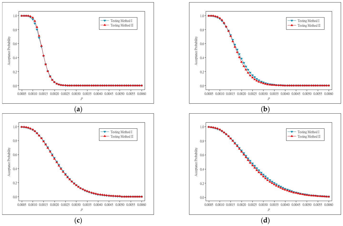
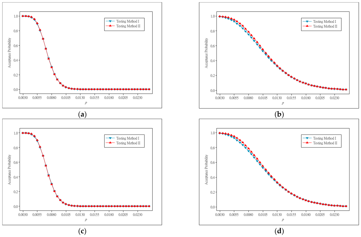
Furthermore, given (α, β) = (0.05, 0.05) and specific quality level combinations, we plot the OC curves of the exponential and Weibull distributions based on the corresponding life acceptance sampling plan parameters under the two different life testing methods. These are used to evaluate the discriminatory power of the life acceptance sampling plans for distinguishing between lots, as shown in Figure 3a–d and Figure 4a–d. For the two different life testing methods, Figure 3a–d illustrate the OC curves under the exponential distribution, while Figure 4a–d illustrate the OC curves under the Weibull distributions.

6. An Illustrative Example

The application of the proposed methodology is illustrated, referring to the case presented in [3]. Real data on electrical insulating fluids is studied, and its lifetime characteristic T with a specified lower lifetime limit L = 1.04 is set. In our example, the scenario that the failure times of electrical insulating fluids follow an exponential distribution is used to simulate the data for product lifetime. Assuming that the quality levels and risks are determined as ($p_{AQL}$, $p_{LTPD}$) = (0.001, 0.005) and (α, β) = (0.01, 0.05), respectively, and Testing Method II is used, then the corresponding parameters can be obtained as (g, s, v, c) = (2, 5, 1, 0.9981) based on Table 3. Thus, two groups are formed, each with a minimum of five items. Testing stops at the fifth failure per group. Now we generate 20 observations and partition the 20 observations into 2 groups randomly, with 10 observations allocated to each group. The data for the two groups are as follows:

Group 1: 1.32, 0.46, 0.01, 0.49, 0.58, 1.68, 1.04, 1.13, 1.01, 1.89.

Group 2: 0.12, 1.27, 1.16, 3.59, 0.43, 0.24, 0.20, 2.14, 4.36, 1.28.

The estimated values of $C_L$ for the two groups, ${\widehat{C}}_{L_1}$ and ${\widehat{C}}_{L_2}$, can be obtained from t₍₁₎, t₍₂₎, …, t₍₅₎ by using Equation (21), which are computed as

$${\widehat{C}}_{L_1}=1-\left[{\displaystyle \frac{s-1}{{\displaystyle {\sum }_{j=1}^s\left(y_{(ij)}+(r-s)y_{(is)}\right)}}}\right]L$$

$$=1-\left[{\displaystyle \frac{5-1}{0.01+0.46+0.49+0.58+1.01+15\times 1.01}}\right]\times 1.2=0.7288,$$

and

$${\widehat{C}}_{L_2}=1-\left[{\displaystyle \frac{s-1}{{\displaystyle {\sum }_{j=1}^s\left(y_{(ij)}+(r-s)y_{(is)}\right)}}}\right]L$$

$$=1-\left[{\displaystyle \frac{5-1}{0.12+0.20+0.24+0.43+1.16+15\times 1.16}}\right]\times 1.2=0.7545.$$

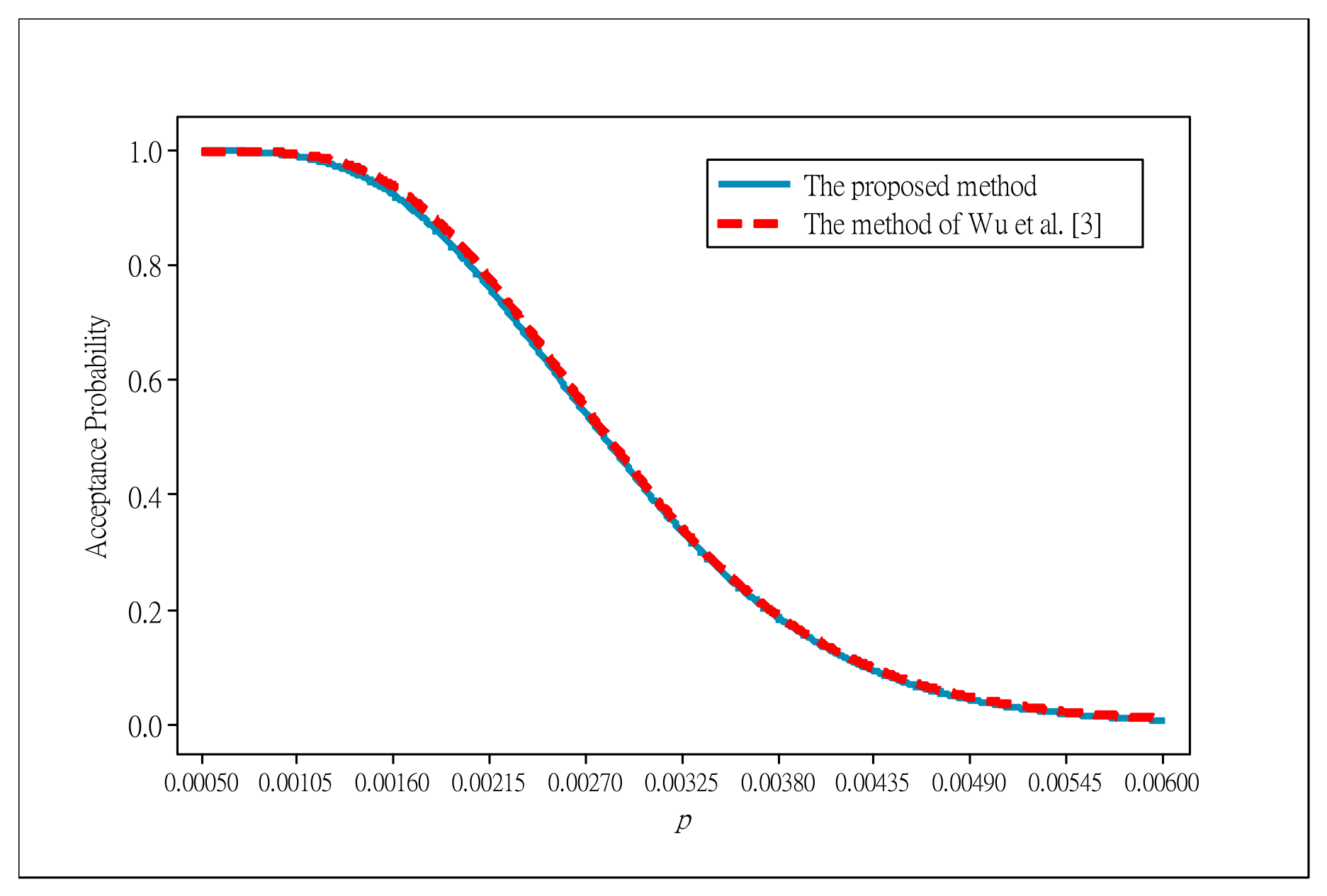
Because none of the two estimated values are larger than the acceptance value c = 0.9981, the lot should be rejected. Additionally, for this case, under the same quality level and risk requirements, our method reaches lot sentencing with only five product failures, whereas [3] requires eight product failures. Consequently, the proposed approach shortens test time. Moreover, under the same quality and risk settings, we compared the lot discrimination capability of our method with that of [3]. Figure 5 shows the OC curves for both approaches. The appearance of the graph indicates that our method almost provides the same lot discrimination as that of [3]. Our proposed method, like the method of [3], provides an efficient sampling plan and can be applied to practical cases.

7. Conclusions

This study developed group-based lifetime acceptance sampling plans using the lifetime performance index. The Weibull distribution was considered the primary reliability model because of its flexibility in describing different failure rate behaviors. The exponential distribution was also included as a simpler benchmark model and as a special case of the Weibull distribution with shape parameter m = 1. The main strengths of the proposed procedures include the integration of group sampling with the lifetime performance index, the derivation of OC-based sampling plans under failure-censored lifetime testing, and the provision of parameter tables for practical implementation. Testing Method I may require a relatively larger number of testing channels (groups) when the sample size per group is small. Testing Method II, on the other hand, requires waiting for the s-th failure, which inherently lengthens the testing time compared to Method I. When multi-channel testing equipment is limited or expensive, Testing Method II is highly recommended; when testing time is the primary bottleneck, Testing Method I should be adopted. For our future research directions, we will focus on the development of cost–time optimization models; the extension of our framework to other lifetime distributions such as lognormal, gamma, log-gamma, and Birnbaum–Saunders distributions; and the integration of historical lot information through multiple dependent state sampling schemes.

References

1. Wu, C.W. An efficient inspection scheme for variables based on Taguchi capability index. Eur. J. Oper. Res. 2012, 223, 116–122. [Google Scholar] [CrossRef]
2. Pearn, W.L.; Wu, C.W. An effective decision-making method for product acceptance. Omega 2007, 35, 12–21. [Google Scholar] [CrossRef]
3. Wu, C.W.; Shu, M.H.; Chang, Y.N. Variable-sampling plans based on lifetime-performance index under Exponential distribution with censoring and its extensions. Appl. Math. Model. 2018, 55, 81–93. [Google Scholar] [CrossRef]
4. Saleh, N.A.; Mahmoud, M.A.; Woodall, W.H. A re-evaluation of repetitive sampling techniques in statistical process monitoring. Qual. Technol. Quant. Manag. 2024, 21, 786–804. [Google Scholar] [CrossRef]
5. Lee, A.H.I.; Wu, C.W.; Wang, T.C.; Kuo, M.H. Construction of acceptance sampling schemes for exponential lifetime products with progressive type II right censoring. Reliab. Eng. Syst. Saf. 2024, 243, 109843. [Google Scholar] [CrossRef]
6. Banihashemi, A.; Wu, C.W.; Amiri, A. Analytical modeling of an acceptance sampling plan with the functional process capability index for circular profiles. Int. J. Prod. Econ. 2025, 288, 109622. [Google Scholar] [CrossRef]
7. Wang, T.C.; Wu, C.W. Adaptive sampling system with quick-switching mechanism indexed by lifetime performance for product reliability verification. Ann. Oper. Res. 2025. [Google Scholar] [CrossRef]
8. Wu, C.W.; Wang, T.C.; Chen, R.H. Development of acceptance sampling plans under time-truncated life test for verifying product reliability using weibull-percentile lifetimes. Reliab. Eng. Syst. Saf. 2025, 261, 111062. [Google Scholar] [CrossRef]
9. Wang, T.C.; Wu, C.W.; Shu, M.H. Developing a failure-censored two-plan sampling system for product reliability validation under the Weibull distribution. Adv. Eng. Inform. 2025, 67, 103584. [Google Scholar] [CrossRef]
10. Chen, K.S.; Chang, T.C. Construction and fuzzy hypothesis testing of Taguchi Six Sigma quality index. Int. J. Prod. Res. 2020, 58, 3110–3125. [Google Scholar] [CrossRef]
11. Yu, C.M.; Huang, T.H.; Chen, K.S.; Huang, T.Y. Construct Six Sigma DMAIC improvement model for manufacturing process quality of multi-characteristic products. Mathematics 2022, 10, 814. [Google Scholar] [CrossRef]
12. Pearn, W.L.; Kang, H.Y.; Lee, A.H.I.; Liao, M.Y. Photolithography control in wafer fabrication based on process capability indices with multiple characteristics. IEEE Trans. Semicond. Manuf. 2009, 22, 351–356. [Google Scholar] [CrossRef]
13. Kang, H.Y.; Lee, A.H.I.; Wu, C.W.; Lee, C.H. An efficient method for dynamic-demand joint replenishment problem with multiple suppliers and multiple vehicles. Int. J. Prod. Res. 2017, 55, 1065–1084. [Google Scholar] [CrossRef]
14. Chen, K.S.; Wang, K.J.; Chang, T.C. A novel approach to deriving the lower confidence limit of indices Cpu, Cpl, and Cpk in assessing process capability. Int. J. Prod. Res. 2017, 55, 4963–4981. [Google Scholar] [CrossRef]
15. Jun, C.H.; Balamurali, S.; Lee, S.H. Variables sampling plans for Weibull distributed lifetimes under sudden death testing. IEEE Trans. Reliab. 2006, 55, 53–58. [Google Scholar] [CrossRef]
16. Aslam, M.; Jun, C.H. A group acceptance sampling plan for truncated life test having Weibull distribution. J. Appl. Stat. 2009, 36, 1021–1027. [Google Scholar] [CrossRef]
17. Aslam, M.; Jun, C.H.; Ahmad, M. A group sampling plan based on truncated life test for Gamma distributions. Pak. J. Stat. 2009, 25, 333–340. [Google Scholar] [CrossRef]
18. Rao, G.S. A group acceptance sampling plans for lifetimes following a generalized Exponential distribution. Econ. Qual. Control 2009, 24, 75–85. [Google Scholar] [CrossRef]
19. Aslam, M.; Pervaiz, M.K.; Jun, C.H. An improved group sampling plan based on time-truncated life tests. Commun. Stat. Appl. Methods 2010, 17, 319–326. [Google Scholar] [CrossRef]
20. Ahmed, B.; Yousof, H. A new group acceptance sampling plans based on percentiles for the Weibull Fréchet model. Stat. Optim. Inf. Comput. 2023, 11, 409–421. [Google Scholar] [CrossRef]
21. Naz, S.; Tahir, M.H.; Jamal, F.; Ameeq, M.; Shafiq, S.; Mendy, J.T. A group acceptance sampling plan based on flexible new Kumaraswamy Exponential distribution: An application to quality control reliability. Cogent Eng. 2023, 10, 2257945. [Google Scholar] [CrossRef]
22. Montgomery, D.C. Introduction to Statistical Quality Control; John Wiley & Sons Inc.: New York, NY, USA, 1985. [Google Scholar]
23. Tong, L.I.; Chen, K.S.; Chen, H.T. Statistical testing for assessing the performance of lifetime index of electronic components with Exponential distribution. Int. J. Qual. Reliab. Manag. 2002, 19, 812–824. [Google Scholar] [CrossRef]
24. Alsaedi, B.S.; Abd El-Raouf, M.M.; Hafez, E.H.; Almaspoor, Z.; Alamri, O.A.; Alanazi, K.A.; Khosa, S.K. Decision-making for the lifetime performance index. Comput. Intell. Neurosci. 2021, 1, 3005067. [Google Scholar] [CrossRef] [PubMed]
25. Wu, S.F.; Lu, J.Y. Computational testing algorithmic procedure of assessment for lifetime performance index of Pareto products under progressive type I interval censoring. Comput. Stat. 2017, 32, 647–666. [Google Scholar] [CrossRef]
26. Wu, S.F.; Song, M.Z. Experimental design for progressive type I interval censoring on the lifetime performance index of Chen lifetime distribution. Mathematics 2023, 11, 1554. [Google Scholar] [CrossRef]
Figure 1. A schematic representation of Testing Method I.
Axioms 15 00588 g001
Figure 2. A schematic representation of Testing Method II.
Axioms 15 00588 g002
Figure 3. The OC curve under the exponential distribution for product life at (α, β) = (0.05, 0.05), and (a) ( p A Q L , p L T P D ) = (0.001, 0.002); (b) ( p A Q L , p L T P D ) = (0.001, 0.003); (c) ( p A Q L , p L T P D ) = (0.001, 0.004); (d) ( p A Q L , p L T P D ) = (0.001, 0.005).
Axioms 15 00588 g003
Figure 4. The OC curve under the Weibull distribution for product life at (α, β) = (0.05, 0.05), and (a) ( p A Q L , p L T P D ) = (0.005, 0.01), and m = 2; (b) ( p A Q L , p L T P D ) = (0.005, 0.02), and m = 2; (c) ( p A Q L , p L T P D ) = (0.005, 0.01), and m = 3 (d) ( p A Q L , p L T P D ) = (0.005, 0.01), and m = 3.
Axioms 15 00588 g004
Figure 5. OC curves under the exponential distribution for the two methods at ( p A Q L , p L T P D ) = (0.001, 0.005) and (α, β) = (0.01, 0.05).
Axioms 15 00588 g005