Article

Method for Automated Decomposition of Monolithic Software Systems Based on Graph Neural Networks

by
Yaroslav Kornaga
1,
Oleksandr Hubariev
1,*,
Serhii Yevseiev
2,
Petro Yablonskyi
3 and
Tetiana Pyrohovska
4
1
Faculty of Informatics and Computer Engineering, National Technical University of Ukraine “Igor Sikorsky Kyiv Polytechnic Institute”, 03056 Kyiv, Ukraine
2
Department of Cybersecurity, National Technical University “Kharkiv Polytechnic Institute”, 61002 Kharkiv, Ukraine
3
Department of Descriptive Geometry, Engineering and Computer Graphics, National Technical University of Ukraine “Igor Sikorsky Kyiv Polytechnic Institute”, 03056 Kyiv, Ukraine
4
Department of Software Engineering for Power Industry, National Technical University of Ukraine “Igor Sikorsky Kyiv Polytechnic Institute”, 03056 Kyiv, Ukraine
*
Author to whom correspondence should be addressed.
Axioms 2026, 15(7), 498; https://doi.org/10.3390/axioms15070498
Submission received: 9 May 2026 / Revised: 10 June 2026 / Accepted: 30 June 2026 / Published: 2 July 2026

Abstract

The purpose of this study is to improve the architectural quality of software systems with microservice architecture by investigating and improving methods for automated transition from monolithic architecture to microservice architecture. The study was performed using methods of static source code analysis, graph theory, algorithms for transforming graph structures (detecting strongly connected components, redundant and cyclic dependencies), cluster analysis algorithms, graph neural networks, as well as multi-criteria assessment of internal cluster consistency and inter-cluster connectivity. The results presented in the study are a comprehensive solution to the scientific problem of ensuring the automated transformation of monolithic software systems into a microservice architecture with controlled inter-service connectivity and a high level of internal consistency of architectural components.

1. Introduction

In recent decades, software developers have increasingly abandoned monolithic systems and switched to microservices. Microservice architecture has better scalability, greater flexibility and ease of maintenance [1]. However, switching from monoliths to microservices is not an easy task as monoliths have hidden dependencies, modules are closely integrated with each other, domain boundaries are virtually absent, and the manual decomposition process of a monolithic system can be lengthy and lead to errors [2]. Therefore, the research and development of automated solutions for the transition from monolithic architecture to microservices are relevant today.
The problem of decomposition has already been studied within various scientific directions [3,4]. Heuristic and metric-oriented approaches [5,6,7] used dependency matrices, connectivity metrics, and rule sets to divide systems into services, which allowed us to achieve a sufficient level of internal consistency of components; however, the resulting clusters only partially corresponded to subject domain boundaries. Later, graph approaches such as Service Cutter, IBM Mono2Micro, DacomiCo, and GDC-DVF began to be used, which used dependency graphs and increased modularity to improve the structural partition of the system.
On the basis of the results of previous studies, more modern approaches have been further developed, which use machine learning methods and aim at automatically detecting syntactic and semantic relationships between components of software systems [8]. Desai et al. in 2021 [9] proposed a graph neural network (GNN) to reduce the impact of abnormal components during refactoring of monolithic applications. Qian et al. in 2023 [10] proposed a deep clustering approach integrating two representations of the system architecture (dual-view fusion) to extract microservices. Yedida et al. in 2023 [11] used deep learning techniques to distribute cloud microservice applications. Sellami et al. in 2022 [12] used the hierarchical DBSCAN clustering algorithm for structural refactoring. Ziabakhsh et al. in 2025 [13] proposed a Mo2oM model—soft clustering (components may belong in part to multiple microservices) based on a graph neural network using deep semantic vector representations.
As a result of using these approaches, it was possible to significantly increase the modularity and semantic coherence of clusters. However, they exhibit sensitivity to data configuration, complexities when combining structural and semantic features, limited efficiency when eliminating redundant intermodular relationships, and difficulties in generalizing training models for heterogeneous software domains [14,15].
The proposed methodology contains several methodological contributions in the field of automated decomposition of monolithic systems into microservices. It provides an adaptive mechanism for the automatic selection of a clustering algorithm based on the structural characteristics of the dependency graph. A mechanism for automatic formation of training labels based on the results of heuristic graph analysis is proposed, which allows the training of a graph neural network without using expertly labeled decompositions or pre-prepared reference data sets. The heuristic procedure is used exclusively at the stage of training data preparation, while after training is completed, the decomposition is performed directly by the graph neural network without repeated application of the heuristic procedure. The proposed approach combines the structural characteristics of the graph, semantic information, and graph-neural representations within a single decomposition process. The model is optimized using a multi-criteria objective function that simultaneously takes into account classification error, cohesion, coupling, and semantic consistency. Together, these components form an adaptive end-to-end framework for automated software decomposition.

2. Materials and Methods

2.1. The Method of Structural Transformation of the Dependency Graph of the Software System

The study proposes a comprehensive approach to the structural analysis of software architecture, which is based on the step-by-step processing of the graph model of the system. At the first stage, the software architecture is analyzed, consisting of several consecutive steps:
  • Construction of an abstract syntax tree (AST).
  • Formation of a directed graph of dependencies between system components.
  • Calculation of the centrality of nodes (to determine structurally important modules of the system).
  • Identification of bridges and points of articulation that ensure the integrity of the architectural model.
  • Determination of weighting coefficients for edges and nodes.
  • Graph structure transformation.
Calculation of the centrality of nodes.
Degree Centrality:
D C ( v ) = D C in ( v ) + D C out ( v ) ,
D C in ( v ) = deg in ( v ) n 1 ,
D C out ( v ) = deg out ( v ) n 1 ,
where:
  • deg in ( v ) is the number of incoming connections of node v;
  • deg out ( v ) is the number of outgoing connections of node v;
  • n 1 is the total number of nodes in the graph excluding node v itself.
Betweenness Centrality:
B C ( v ) = s v t σ s t ( v ) σ s t ,
where:
  • σ s t is the total number of shortest paths between nodes s and t in the graph;
  • σ s t ( v ) is the number of such shortest paths passing through node v.
Identification of bridges and points of articulation that ensure the integrity of the architectural model.
First, the critical nodes of the dependency graph of the software system are determined. For this, a threshold analysis is used, according to which node v is considered critical if the following condition holds:
D C ( v ) > μ D C + σ D C ,
or
B C ( v ) > μ B C + σ B C ,
where:
  • μ D C and σ D C are the mean value and standard deviation of Degree Centrality;
  • μ B C and σ B C are the mean value and standard deviation of Betweenness Centrality.
The critical threshold value is determined dynamically for each analyzed project based on the statistical distribution of centrality values.
After identifying critical nodes, a depth-first search (DFS) algorithm is applied, which allows us to identify structurally important elements of the dependency graph by analyzing their impact on the overall connectivity of the system. Since the detection of bridges and articulation points is defined for undirected graphs, this analysis is performed on the undirected representation of the dependency graph.
During the DFS traversal, two parameters are calculated for each vertex v:
  • d f s [ v ] —the discovery time of node v;
  • l o w [ v ] —the minimum discovery time of any vertex reachable from v through DFS tree edges and back edges, including v itself.
Calculating these values is a key step in DFS analysis based on low-link values, which is used to detect bridges and articulation points. The value of l o w [ v ] is determined as follows:
l o w [ v ] = min d f s [ v ] , min w c h i l d r e n ( v ) l o w [ w ] , min u b a c k - e d g e s ( v ) d f s [ u ] ,
where:
  • d f s [ v ] is the discovery time of node v during DFS;
  • l o w [ w ] is the low value of a child node w of vertex v in the DFS tree;
  • d f s [ u ] is the discovery time of a node u connected to v by a back edge.
The edge e ( u , v ) is considered a bridge in the dependency graph if the following condition holds for the descendant node v:
l o w [ v ] > d f s [ u ] ,
This means that vertex v and its subtree cannot be reached from the rest of the graph without the edge e ( u , v ) ; therefore, removing this edge disconnects the graph into separate components.
Vertex v is defined as an articulation point in the following cases:
  • If vertex v is the root of a DFS tree and has more than one child.
  • If the following condition holds for any child:
l o w [ c h i l d ] d f s [ v ] .
This suggests that after removing vertex v, its child will lose its connection to other parts of the graph.
Bridge edges are denoted as critical connections between autonomous subgraphs, the removal of which leads to the rupture of the graph. Bridge edges in the dependency graph are not removed because they are critical to preserving system connectivity, but are seen as natural boundaries between future microservices because they connect autonomous subgraphs through a minimal number of interactions.
Articulation points are nodes through which communication between several subsystems is carried out, and such nodes should be marked as central routing elements or isolated into separate clusters to prevent excessive connectivity.
Determination of weighting coefficients for edges and nodes.
Formula for calculating the weight of an edge:
W ( e i j ) = w k ,
where:
  • w k —weight of the corresponding type of edge.
Table 1 presents the edge types in the dependency graph, their assigned weight values, and descriptions of the corresponding relationships between software components.
The weights given in Table 1 reflect the relative strength of different types of architectural dependencies. Inheritance relationships receive the highest weight because they create strong structural coupling between components. The use of classes represents a direct implementation dependency and therefore also receives a relatively high weight. Meanwhile, function calls, use of interfaces, and interaction through a shared database receive lower weights because they typically reflect weaker or more indirect forms of coupling. The weights were chosen heuristically based on generally accepted principles of software architecture and should be considered as empirical indicators of the strength of dependencies rather than mathematically derived constants.
The node weight W ( v ) allows for a quantitative assessment of the architectural significance of a component, taking into account:
  • Its incoming and outgoing connections;
  • Its role in data flow between other modules;
  • Its frequency of use as a dependency in other modules.
Formula for calculating the node weight:
W ( v ) = D C in ( v ) + D C out ( v ) + B C ( v ) ,
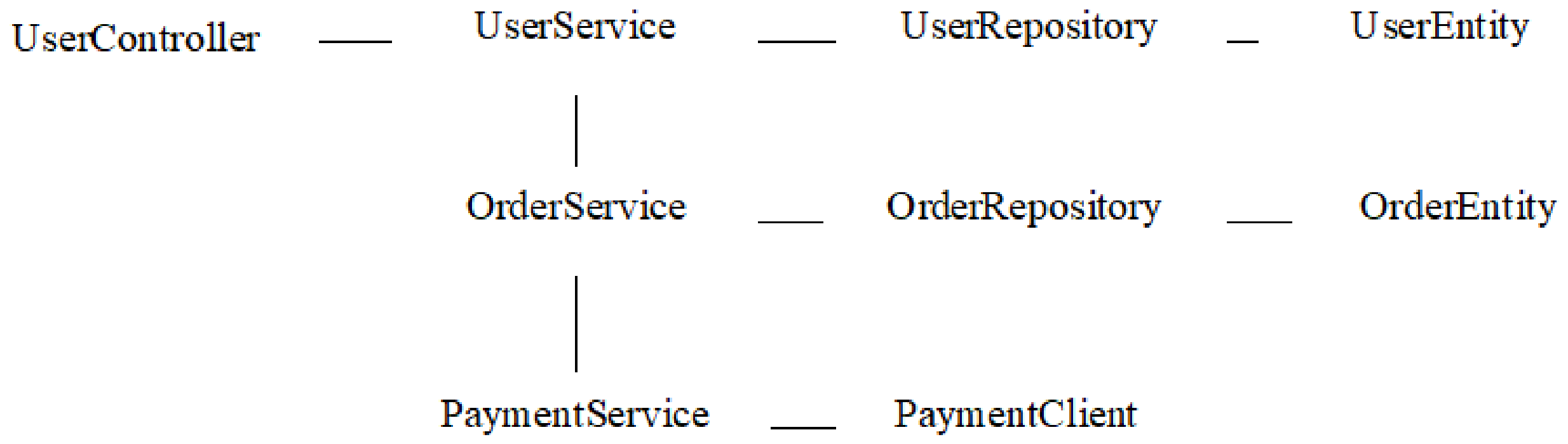
To illustrate the graph-theoretic concepts used in the proposed approach, Figure 1 shows a simplified dependency graph of a hypothetical software system. The example demonstrates typical architectural relationships between controllers, services, repositories, entities, and external clients. Such a graph is used to explain centrality metrics, bridges, and articulation points and their role in the process of structural analysis of software architecture.
In the given example, the UserService node is a structurally important element as it connects several functional subsystems, which leads to a high Degree Centrality value. The UserService and OrdersService nodes also belong to a significant number of shortest paths between other components of the graph, which leads to increased values of Betweenness Centrality. The connection between UserService and OrdersService can be considered a bridge since its removal leads to a disruption of the connectivity of part of the graph. Similarly, the UserService node can act as an articulation point, since its removal increases the number of connected components of the graph. Such structural characteristics are used to identify critical elements of the architecture before performing a decomposition of the software system.
To illustrate the impact of dependency weights on the graph structure, different types of relationships should be assigned different weights according to Table 1. The relationship UserRepository → UserEntity has a weight of w = 0.7 (class usage), the relationships OrderService → PaymentService and UserService → OrderService have a weight of w = 0.5 (function call). This weighting allows us to take into account the different architectural significance of the dependencies when constructing and analyzing the graph.
Graph structure transformation.
Using the results of the analysis carried out in the previous stages, a process of structural transformation of the graph is implemented, which includes detection and removal of weak and redundant connections, removal of cyclic dependencies, and combining nodes into more connected and structurally stable components.
In the first step, a search is made for subgraphs with high internal connectivity (strongly connected components (SCC)). Detection of SCC allows us to identify cyclic dependencies between modules, to see high cohesion groups that can be considered as single logical blocks, and to detect structural antipatterns, for example, when several modules constantly interact with each other (call methods, transmit data), forming a closely related set of dependencies.
To identify strongly connected components (SCCs) representing cyclic dependencies in the graph, Tarjan’s Algorithm is used:
S C C ( G ) = i = 1 k G i ,   G i = ( V i , E i ) ,  
where:
  • S C C ( G ) is the set of all strongly connected components in the graph, where for every pair of vertices u , v V i , there exists a directed path from u to v and a directed path from v to u;
  • G i = ( V i , E i ) is a separate subgraph (one SCC);
  • k is the number of SCCs found.
After identifying strongly connected components (SCC), it is necessary to determine their density. The density of a component, D S C C , indicates how tightly the nodes within the subgraph are interconnected.
The density is calculated using the formula:
D S C C = | E S C C | | V S C C | · ( | V S C C | 1 ) ,
where:
  • | E S C C | is the number of edges within the SCC;
  • | V S C C | is the number of nodes within the SCC.
To identify strongly connected components with increased density, it is necessary to compute a global density threshold, D threshold .
Threshold determination:
D threshold = D ¯ + σ D ,
SCC with D S C C < D threshold are weakly connected (any cycle present is likely non-critical).
SCC with D S C C D threshold are dense and considered as potential candidates for transformation.
To calculate the set of all simple cycles in a directed graph without duplications, this study uses Johnson’s algorithm, which is based on depth-first search (DFS) and is optimized by reducing the search space.
Once all cycles have been detected, the least important connections must be removed (considering the importance of both the connections themselves and the nodes they connect) for the graph to become acyclic.
For this, a combined metric is proposed that takes into account the weight of the connection, the weight of the target node, and the centrality of the target node (structural role in the graph).
Formula for selecting an edge to break a cycle:
e * = min e i j C W ( e i j ) W ( v j ) + B C ( v j ) + ε ,
where:
  • e i j —a directed edge from node v i to vertex v j ;
  • C—the set of edges forming a specific cycle in the graph;
  • W ( e i j ) —edge weight;
  • W ( v j ) —node weight of v j ;
  • B C ( v j ) —the centrality of node v j in the graph structure;
  • ε 1 —a constant to avoid division by zero.
In the next step, it is necessary to evaluate which of the strongly connected components (SCCs) should be combined into a single logical node, which will simplify the structure of the graph.
For each SCC, it is necessary to compute the weighted average strength of the connections between its nodes, taking into account the importance (weighting coefficients) of the nodes themselves.
To this end, we compute the average weight of internal edges within the SCC:
W S C C = 1 | E S C C | e i j E S C C W ( e i j ) W ( v i ) + W ( v j ) 2 ,
where:
  • E S C C —the set of edges in the SCC;
  • e i j —an edge between nodes v i and v j in the SCC;
  • W ( e i j ) —the weight of the edge between vertices v i and v j ;
  • W ( v i ) and W ( v j ) —node weighting coefficients representing the importance or influence of each node;
  • W ( v i ) + W ( v j ) 2 —the average weight of the nodes connected by edge e i j .
To identify SCCs with significantly higher internal connectivity compared to others, which can be merged into a single node, an edge weight threshold is computed:
T W = μ W + σ W ,
where:
  • T W —edge weight threshold.
  • μ W —the mean value of W S C C calculated across all detected strongly connected components;
  • σ W —the standard deviation of W S C C values calculated across all detected strongly connected components.
SCCs in which the average weight of the internal edges W ¯ S C C k exceeds the threshold T W are considered as candidates to join into a node because they exhibit high internal cohesion.
Additionally, to reduce excessive coupling between components of the software system, it is necessary to identify and eliminate redundant edges that duplicate information flow paths already established indirectly through other components. Specifically, if a direct connection W direct exists between two modules, and an indirect connection W indirect is also present, the redundant direct connection may be removed. Indirect paths are defined as simple directed paths from u to v whose length is greater than one edge and does not exceed four edges. The total indirect weight is calculated as the sum of the edge weights for all such paths.
Formula for checking a redundant edge:
W direct < W indirect ,
If this condition holds, the direct edge is removed.
Resulting graph after transformation:
G = ( V , E ) ,
where G = ( V , E ) is a subset of nodes and edges after structural transformation.
E = E { e i j W ( e i j ) < T } ,
where only the most important edges are preserved.
As a result of performing a given sequence of operations (removing cycles, merging strongly connected components, and eliminating redundant connections), a dependency graph G = ( V , E ) is formed, which preserves only structurally important connections between components.
Such a graph is characterized by a lower density and a better balanced topology, in which there are no information duplications, better visibility of modular boundaries and which is the basis for further high-precision clustering.

2.2. Dynamic Selection Method of the Clustering Algorithm

In the second stage, the graph is subject to further clustering. Clustering makes it possible to automatically isolate logically coupled subsystems which, given technological and architectural constraints, can be converted into independent microservices.
A directed dependency graph of a software system serves as the initial model for solving the clustering problem.
Let C = { C 1 , C 2 , , C k } be a partition of the set V into k disjoint subsets (clusters), such that:
i = 1 k C i = V , C i C j = , i j ,
Clustering is considered successful if:
(1)
the intra-cluster connectivity (cohesion) within each C i is maximized;
Cohesion measures how strongly the components within a service are related to each other, how many internal connections exist between them and how consistently they contribute to a common function.
For each cluster C, cohesion is defined as:
C o h e s i o n ( C ) = u , v C ,   u v W ( u , v ) | C | ( | C | 1 ) ,
where:
  • W ( u , v ) —the weight of the edge between classes u and v;
  • | C | —the number of elements in the cluster.
(2)
the inter-cluster connectivity (coupling) between C i and other C j is minimized.
Coupling measures the number of external connections a service has and the extent to which it depends on other clusters.
C o u p l i n g ( C ) = u C v V C W ( u , v ) ,
where:
  • W ( u , v ) —the weight of the external edge between classes u and v.
Thus, coupling is defined as the total weight of all outgoing dependencies from a cluster to other clusters.
This is formulated as a multi-criteria problem:
max C i = 1 k C o h e s i o n ( C i ) C o u p l i n g ( C i ) ,
Thus, the graph G partitioning is carried out into such clusters C i , which are characterized by the highest value of the clustering quality metric.
Semantic consistency is used to estimate how much components within the same service belong to a common subject area and perform close functional roles, and unlike structural metrics (cohesion and coupling), which analyze only the dependency graph, semantic homogeneity allows checking the correspondence of clusters to logical domain boundaries. The structure of the graph can vary significantly for different software systems (density, size, the direction of edges in the graph, availability of shared resources, etc.), so the use of a single clustering algorithm for all cases is limited. Instead, a dynamic approach to choosing a clustering algorithm is proposed, which is based on local characteristics of the graph: number of nodes | V s | , density D ( S ) , local FanOut, Shared Resource Ratio (SRR), and betweenness centrality of nodes B C ( v ) .
Table 2 presents the dynamic clustering algorithm selection strategy based on graph metrics, including the corresponding conditions and the recommended clustering method for each graph structure scenario.
The threshold values given in Table 2 were chosen empirically during research experiments and should be interpreted as practical decision-making criteria rather than as theoretically optimal limits.
The absolute values of the decomposition quality metrics depend not only on the chosen clustering algorithm but also on the complexity, density, structure of relationships, and existing architectural dependencies of the software system under study. Therefore, the proposed mechanism for dynamic algorithm selection is aimed at determining the most suitable clustering strategy for a specific structure of the dependency graph. Its goal is to adapt the decomposition process to the specifics of the analyzed system rather than providing predetermined values of the quality metrics.

2.3. Cluster Structure Refinement Method

To improve the architectural structure and strengthen modular insulation, it was proposed to apply a model that will take into account the structural and semantic indicators of the quality of cluster partitioning.
Thus, the problem reduces to finding a partition C 1 , C 2 , , C K , that maximizes the overall objective function:
max ( C 1 , , C K ) 1 K i = 1 K C o h e s i o n ( C i ) 1 | E | i j C o u p l i n g ( C i , C j ) , subject to : i ,   S e m ( C i ) δ ,
where:
  • δ —fixed threshold.
To implement the model, iterative search is used to gradually improve the initial partitioning of system components, where at each iteration one of the nodes of the graph is randomly selected and the feasibility of moving it to one of the neighboring clusters is checked. The proposed strategy limits the search space within the structurally close environment, which ensures better convergence of the algorithm due to minimal interference with the general structure.
To prevent the degradation of architectural integrity, the model sets a limit—the node cannot be moved to a new cluster if the semantic consistency of the target cluster then becomes lower than the given threshold δ = 0.5 .
The quality assessment of each potential change is carried out on the basis of a weighted metric, which is formally given as:
t e m p _ s c o r e = 2.0 · c o h e s i o n 0.1 · c o u p l i n g
In a given function, a factor of 2.0 is applied for cohesion to form tightly coupled subsystems, whereas the coefficient of 0.1 for coupling allows us to maintain control over modular insulation and avoid excessive fragmentation of clusters.
The coefficients were chosen empirically to enhance the effect of cohesion improvement during local node movement while preventing coupling-related changes from dominating the temporal estimate. They should be interpreted as heuristic calibration parameters rather than theoretically derived constants.

2.4. Graph Neural Network-Based Decomposition Model

In the next stage of the research, a graph neural network model was employed to automate the software system decomposition process.
A system, represented as a graph of dependencies between its components, shows a network structure (nodes as classes or modules, edges as calls, dependencies or interactions between them) and requires models that can process not only feature vectors but also take into account the context of the node’s placement in the graph structure (topological environment and types of connections with other nodes).
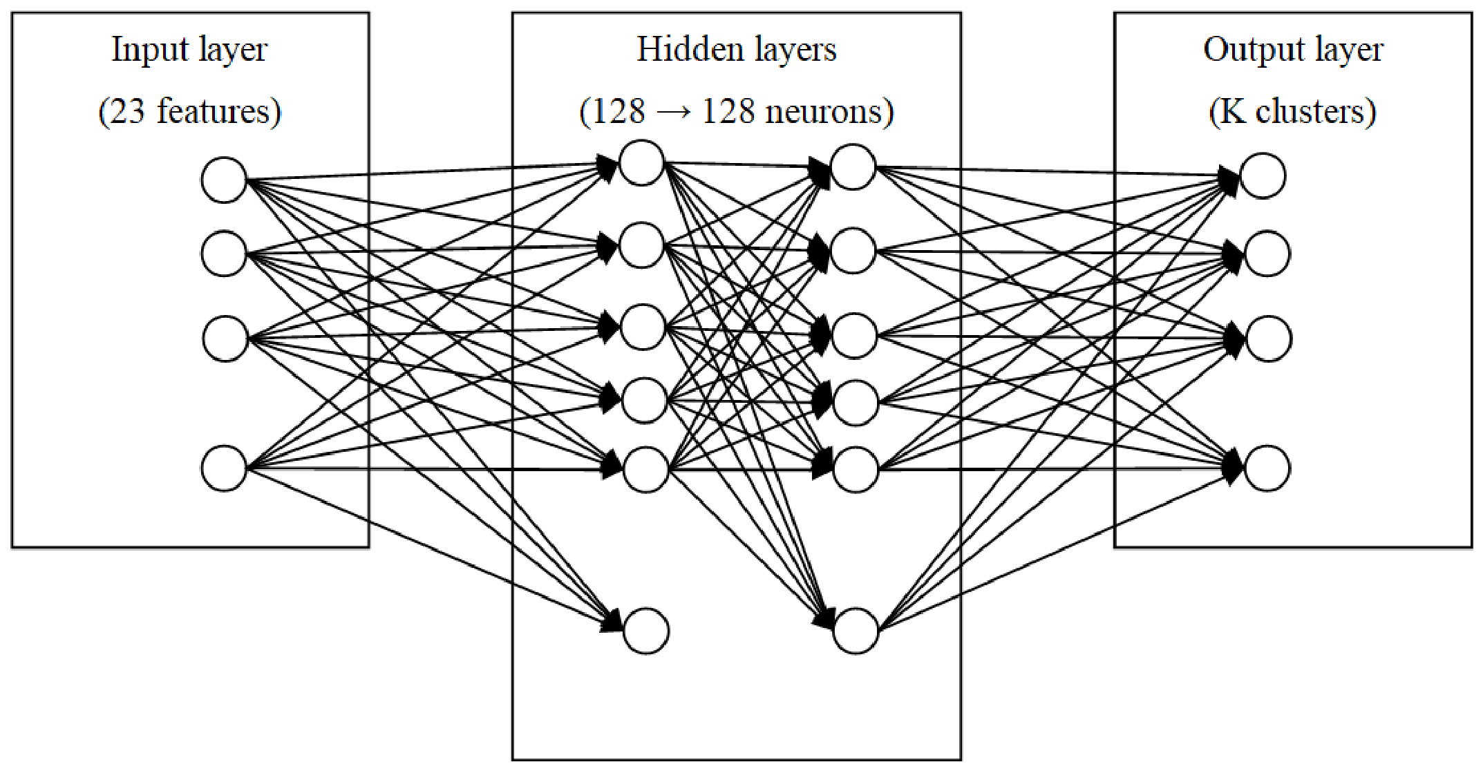
Therefore, a modification of the Graph Convolutional Network (SimpleGCN) was chosen for modeling, which works directly on the graph structure and aggregates information from the local context of each node through a normalized adjacency matrix. This model allows learning internal representations of components, taking into account their own properties and the structural environment in which they function.
The neural model is presented in Figure 2.
A two-layer architecture was chosen because it provides a balance between depth of analysis and maintaining feature clarity. The first layer of the GCN processes the closest connections between classes that form the local structure, while the second layer takes into account interactions at a distance of two steps (connections between neighboring subsystems, where domain logic manifests itself). This is enough for the network to identify important architectural context, but at the same time, it does not average features, which would lead to a blurring of distinctions between classes.
The width of both layers is set to 128 hidden components. This is sufficient to reproduce medium- and large-scale architectural structures, while limiting the risk of overfitting.
For each node of the graph, a feature vector was constructed, which included structural and semantic characteristics. The following structural features were added:
  • In-degree centrality of the node;
  • Out-degree centrality of the node;
  • Betweenness centrality of the node;
  • Local clustering coefficient:
    C ( v ) = 2 e v k v ( k v 1 ) ,
    where:
    • e v —the number of edges between the neighbors of node v;
    • k v —the number of neighbors.
  • PageRank coefficient:
    P R ( v ) = 1 d | V | + d u N ( v ) P R ( u ) deg ( u ) ,
    where:
    • d—damping factor;
    • | V | —the number of nodes in the dependency graph;
    • N ( v ) —the set of incoming neighbors of vertex v, i.e., vertices from which edges are directed to v;
    • deg ( u ) —the number of edges between node u and other components of the dependency graph.
  • Node weight;
  • A binary feature indicating resource usage, which captures whether a component participates in data access operations and is important for modeling data sharing across clusters:
    i s _ r e s o u r c e v = 1 , if   component   v   represents   a   common   data   layer   element   used   by   multiple   domain   components , 0 , otherwise .
When propagating information through a graph, the neural network takes into account the node type and the weight of the connection and forms a representation of each component that takes into account its structural and data context. If the components of the system are connected by the same resource, their vector representations converge, which indicates a potential dependency through a common data model. Due to the lower weight, resource connections do not prevail over business logic connections, and the neural network forms service boundaries that take into account both programmatic interaction and connections to the database.
After receiving the services, an analysis of the distribution of resources between them is performed; for each resource, the service that has the closest connection to the resource is determined by calculating the total weight of the connections between the component and the corresponding resource. Such a service is considered the owner of the resource; however, if the resource is used equally by several services, then such a case is recorded as a conflict and requires additional analysis during migration.
Semantic features were also included in the vector representation of nodes. Class names were converted to lowercase and compared to a predefined dictionary of domain tags using a case-insensitive substring search. If a matching tag was found in the class name, the node was assigned a binary semantic vector that reflected its semantic category. In the absence of a match, a null vector was used.
The semantic representation is given as a vector:
s ( v ) = ( s 1 , s 2 , , s k ) ,   s i { 0 , 1 } ,
where k corresponds to the number of defined semantic categories.
The loss function was enriched with three structural and semantic components. The first component is aimed at increasing the density of connections between nodes (cohesion) within each cluster. The second component is aimed at reducing inter-cluster connections (average FanOut). The third component is aimed at increasing semantic consistency (estimated as the average cosine deviation between vector representations of nodes of the same cluster).
Multi-criteria loss function:
L = C E + F a n O u t a v g C o h e s i o n S e m a n t i c C o n s i s t e n c y ,
where:
  • C E —cross-entropy, which measures the difference between the predicted and target probability distributions of clusters;
  • F a n O u t a v g —average number of output dependencies of cluster nodes;
  • C o h e s i o n —average number of internal connections between nodes of the same cluster;
  • S e m a n t i c C o n s i s t e n c y —determined based on the vector similarity of class names, tags, and attributes, i.e., the extent to which objects in the same cluster have a similar subject entity.
C o h e s i o n and S e m a n t i c C o n s i s t e n c y are presented as normalized values in the range [0, 1]. F a n O u t a v g is logarithmically scaled before aggregation to reduce the impact of extreme values.

3. Results

3.1. Experimental Setup

In order to test the proposed methods of structural analysis of software systems, a test environment and an experimental stand were built. The Google Colaboratory cloud environment (Google Colab) was used for the experiments, which provides an integrated Python 3.12.13 environment with pre-installed libraries for data processing and the ability to restart experiments.
To verify the proposed approach and methods of automated transformation of software architecture, experimental studies were conducted using graph models obtained from the source code of an industrial logistics process management system implemented in Java using the Spring framework. The system is a large-scale monolithic corporate application containing several interconnected business modules. Due to confidentiality and intellectual property protection restrictions, the source code cannot be made public. The experiments were aimed at assessing the quality of the resulting cluster partition and checking the feasibility of dynamically selecting a clustering algorithm that depends on the structural characteristics of the dependency graph.
The experimental evaluation combined a detailed study of an industrial software system with a comparative evaluation on a set of test software systems. Accordingly, the presented metrics should be interpreted as indicators of the quality of decomposition for the studied software systems and not as statistical estimates obtained on the basis of multiple experimental tests.

3.2. Experimental Evaluation of Dynamic Clustering Algorithm Selection

To evaluate the method, graphs were constructed for 30 projects of varying scale. On the same graphs, all selected clustering algorithms were run in turn. Coupling and cohesion were calculated for each result. The algorithm that gives the best balance of these indicators is considered the most suitable for this project.
In parallel with this, the method of dynamic selection of the clustering algorithm was used, and it was checked whether this selection coincides with the most suitable algorithm that was found by exhaustive search. Next, it was calculated how often the method accurately chooses the most suitable algorithm, as well as how often the correct algorithm falls into the top two options. Separately, it was analyzed how much the indicators of coupling and cohesion deteriorate or improve if the choice was not the best.
Table 3 presents the results of the experimental evaluation of the dynamic clustering algorithm selection method for different graph size groups, including Top-1 and Top-2 accuracy, number of mistakes, and average deviations of cohesion and coupling values.
According to the results of an experimental study, the dynamic selection method provided an exact match with the result of a complete search in 73.3% of cases, while in 86.7% of cases the correct algorithm was among the two best options. The mean deviation of cohesion at the non-best choice is negligible (about −0.004), while the mean increase in intercluster connectivity is about 0.14, which confirms the stability of the method regardless of the size of the graph.

3.3. Experimental Evaluation of the Graph-Based Decomposition Approach

In the first step, a syntactic and semantic analysis of the source software code is performed to construct a graph of dependencies between classes. 518 files were processed (excluding test files) and a directed system graph was formed:
  • Number of nodes (classes/modules)—345;
  • Number of oriented edges (dependencies)—641.
After applying the proposed graph structural transformation method, the number of edges decreased to 452, that is, 189 edges were removed from the graph (about 29% of the original number of edges).
By removing the edges, the graph has become less cyclic and the noise level has decreased, which should improve the quality of clustering.
At the next stage, the structural characteristics of the directed graph were calculated:
  • Global graph density— 0.0038 ;
  • F a n O u t a v g 1.310 ;
  • Shared Resource Ratio (SRR)— 0.0638 ;
  • Normalized betweenness centrality ( B C ¯ n o r m ) 0.000726 .
Based on the obtained metrics, the graph can be classified into the following set of conditions:
B C ¯ n o r m < 0.05 D ( G ) < 0.1 | V | > 300 F a n O u t a v g < 2 S R R < 0.2
According to the classification scheme for selecting clustering algorithms, Label Propagation is the most suitable method for this type of graph.
After applying this clustering algorithm, 32 clusters were formed and cohesion, coupling and semantic consistency were calculated to assess the quality of the decomposition.
The average level of cohesion in clusters is only 0.0682. This indicates that clusters have weak internal connectivity of components, that is, the number of strong structural or functional dependencies between classes grouped into one module is low.
Coupling is 119.0, meaning that the system has many external connections between clusters, making it difficult for modules to develop independently, and it is a source of violations of the principle of loose coupling.
The semantic consistency of clusters is 0.4883, that is, clusters partially correspond to the functional content of software components, but there are also a significant number of modules that belong to different domains.

3.4. Evaluation of Cluster Structure Refinement Method

The same industrial software project that was used in the study of the heuristic graph approach was used to evaluate the cluster structure improvement method. After applying the improvement method, the average cohesion value increased from 0.0682 to 0.0752, the total number of intercluster dependencies decreased from 119.00 to 88.20, and the semantic coherence value of the clusters increased from 0.4883 to 0.6358.
The results obtained confirm the feasibility of applying the cluster structure improvement stage after the initial graph decomposition. The results generated using the heuristic graph approach and the cluster improvement method are further used to form the reference decomposition and cluster labels necessary for training the graph neural network.

3.5. Evaluation of the Graph Neural Network-Based Decomposition Model

To train the graph neural network, open-source Java projects were used as a training set: Spring PetClinic, Broadleaf Commerce, OpenMRS Core, and Apache OFBiz (Project repositories: https://github.com/spring-projects/spring-petclinic (accessed on 29 June 2026), https://github.com/BroadleafCommerce/BroadleafCommerce (accessed on 29 June 2026), https://github.com/openmrs/openmrs-core (accessed on 29 June 2026), https://github.com/apache/ofbiz-framework (accessed on 29 June 2026).), covering different architectural approaches and scales (from 250 to over 600 classes).
The graph neural network was trained on a graph where each node had a predefined cluster membership, i.e., the system learned to reproduce the clustering structure that was obtained in the previous steps using a heuristic approach.
The goal of training the model was to form a vector representation of the nodes of the architectural graph, in which nodes from the same structural or functional context are located closer to each other, and nodes from different contexts are located further apart in the feature space. By using a modified loss function, the model learned a generalized representation of the structure of the software system rather than reproducing specific cluster labels.
As a result of training a graph neural network, a space of vector representations (embeddings) was obtained, where each node of the graph corresponds to a vector that summarizes its structural characteristics, semantic properties, and the context of interaction with other nodes in the dependency graph.
In the testing phase, the model was applied to an industrial project that was used to evaluate the application of the heuristic approach. For the test project, an architectural dependency graph was first constructed and initial feature vectors of nodes were created, then the model performed a direct traverse of the graph and calculated class embeddings, which served as input data for the subsequent clustering phase.
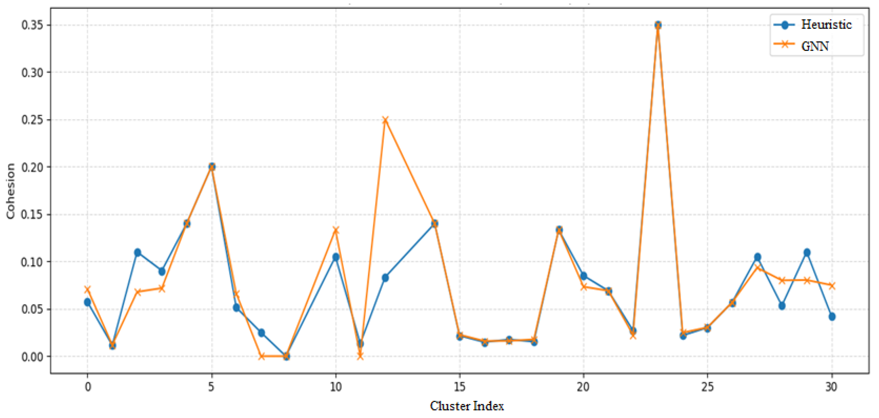
After applying the neural network, the semantic consistency improved compared to the heuristic approach. Its value increased from 0.4883 to 0.6358, which means that the semantic homogeneity of components belonging to the same domain increased. It can be concluded that the model can not only preserve the structure of the initial clustering but also improve it in terms of subject consistency. The average cohesion value, compared to the initial clustering, increased across the system from 0.0752 to 0.0890, or 18.3%. This means that the internal density of connections within the clusters has increased. Comparison of the internal consistency values of individual clusters for heuristic and GNN approaches is presented in Figure 3.
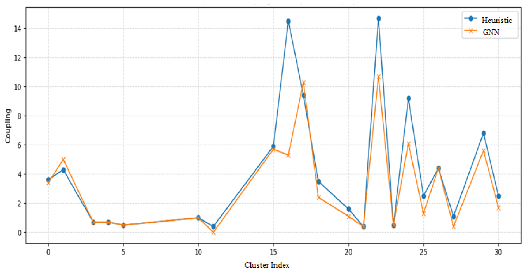
An even more important result was the reduction in coupling. The average coupling decreased from 4.20 to 3.36 (i.e., by 20%), and the total number of inter-cluster connections in the system decreased from 88.2 to 67.2, i.e., by 23.8%. Comparison of the inter-service connectivity values of individual clusters for heuristic and GNN approaches is presented in Figure 4.

3.6. Comparative Analysis with Existing Approaches

At the next stage, a comparative analysis of the proposed approach with modern graph methods—CoGCN, DEEPLY, HyDEC, GDC-DVF and Mono2Micro—was carried out. Following the experimental protocol described in the literature, the basic methods were evaluated using implementations and hyperparameter settings recommended by their authors. This ensured consistent experimental conditions and correct comparison of the obtained results. The Structural Modularity (SM) and Inter-Call Percentage (ICP) metrics are used for comparison [13].
The SM metric is used to assess the structural quality of a monolithic system decomposition and characterizes the balance between a cluster’s cohesion and intercluster dependencies. Higher SM values correspond to better structural modularity of the decomposition.
The value of the metric is determined by the formula:
S M = 1 k i = 1 k e i n i 2 2 k ( k 1 ) i = 1 k 1 j = i + 1 k e i j 2 n i n j ,
where:
  • k—the number of clusters;
  • e i —the number of edges inside cluster i;
  • n i —the number of classes in cluster i;
  • e i j —the number of edges between clusters i and j;
  • n j —the number of classes in cluster j.
Inter-Call Percentage (ICP) is used to evaluate the degree of interaction between clusters and represents the proportion of inter-cluster calls relative to the total number of calls in the system. Lower ICP values indicate weaker coupling between clusters and a higher quality decomposition.
The metric is computed as follows:
I C P = E e x t e r n a l E i n t e r n a l + E e x t e r n a l ,
where:
  • E e x t e r n a l —the total number of calls (edges) between different clusters;
  • E i n t e r n a l —the total number of calls (edges) within clusters.
The methods were applied to an industrial project. The results are presented in Table 4.
The results obtained for the industrial project demonstrate the superiority of the proposed approach over all the compared methods in terms of structural modularity and intercluster connectivity. SM = 0.1295 is higher than CoGCN (0.027), DEEPLY (0.040), GDC-DVF (0.041) and Mono2Micro (0.030) and also exceeds the result of HyDEC (0.080). ICP = 0.2950 is the lowest among all the considered approaches. CoGCN (0.559), DEEPLY (0.546), Mono2Micro (0.658) and HyDEC (0.425) demonstrate a significantly higher level of intercluster dependencies.

3.7. Complexity and Scalability Analysis

The proposed approach works with a directed dependency graph containing V nodes and | E | edges. Graph construction, dependency filtering, and most of the preprocessing and analysis steps of the graph are performed with linear or quasi-linear complexity relative to its size. A sparse representation is used to store the graph, so the memory requirements are O ( | E | ) for the graph structure and O ( V · d ) for the node feature matrix, where d is the size of the feature vector.
The SimpleGCN model propagates information directly along the edges of the dependency graph. For each layer of the graph convolution, the computational complexity is proportional to the number of edges in the graph and the size of the hidden representation. Thus, the total training complexity is estimated as O ( epochs · | E | · h ) , where h is the size of the hidden layer. Since dependency graphs of software systems are usually sparse, computational costs grow mostly linearly with increasing number of dependencies, which makes the proposed approach suitable for analyzing large enterprise-level software systems.

4. Discussion

The obtained experimental results confirm the initial working hypothesis that the complex structural use of graph analysis, dynamic clustering algorithm selection, cluster structure improvement, and graph neural network provide an increase in the quality of decomposition of monolithic software systems on a microservice.
The initial decomposition of the software system was obtained using a heuristic approach that used the structural characteristics of the dependency graph and a set of rules for forming initial clusters. For the industrial system under study, this approach provided a cohesion value of 0.0682, a total number of intercluster dependencies of 119.00, and a semantic consistency of 0.4883. The results obtained confirm the ability of the heuristic approach to form an initial decomposition, but there remains significant potential for improving both the structural and semantic quality of the clusters.
At the next stage, a cluster improvement procedure was applied. The application of the cluster structure improvement method made it possible to significantly increase the internal connectivity of modules and reduce the number of external dependencies between clusters. The average value of cluster cohesion increased from 0.0682 to 0.0752, which means strengthening the internal structural integrity of clusters; coupling decreased from 119.00 to 88.20, which means increasing modular isolation; at the same time, the semantic consistency of clusters increased from 0.4883 to 0.6358, which confirms a better alignment of the structural decomposition with the domain logic.
Further application of the graph neural model to an industrial software project allowed us to take into account not only the structural characteristics of the dependency graph but also the semantic features of the software components. As a result, the proposed approach provided higher cohesion compared to the heuristic method (0.0890 vs. 0.0752, 18.3%), which had a lower number of intercluster dependencies (67.2 vs. 88.2, 23.8%). The results obtained indicate that the use of a graph neural network allows us to more effectively identify hidden connections between software components and form a higher-quality decomposition of the software system.
Compared to the basic and modern approaches, the proposed method demonstrated consistently higher values of structural modularity (SM) and lower inter-service coupling (ICP) indices, which indicates a more balanced and architecturally justified decomposition.
For an industrial software project, the proposed approach achieved an SM value of 0.129, which significantly exceeds the results of alternative methods, in particular IBM Mono2Micro (0.030), CoGCN (0.027), DEEPLY (0.040) and GDC-DVF (0.041). The structural modularity index characterizes the level of internal integrity of the formed services while minimizing unnecessary dependencies between them. Accordingly, the growth of this indicator indicates that the defined service boundaries better correspond to the real business functions and technical areas of responsibility of the system. This is especially important for corporate information systems, where poor-quality decomposition often leads to excessive inter-service interaction, duplication of logic and complication of further support.
At the same time, the proposed method demonstrated the lowest ICP value (0.295) among all the compared approaches. Since this indicator characterizes the level of structural dependence between the allocated services, its reduction means a reduction in the number of inter-service calls and a higher level of functionality encapsulation. From a practical point of view, this can provide better scalability, simplify independent deployment of components, and reduce the risk of cascading failures in a distributed environment. Compared to Mono2Micro (0.658) and CoGCN (0.559), the obtained advantage is significant, which confirms the limitations of approaches focused exclusively on clustering or similarity of components without taking into account hidden structural dependencies.
From the perspective of previous studies, the results obtained are consistent with the current trend of using graph models for analyzing software architectures. Early methods, such as Service Cutter, mainly relied on manually defined criteria for the relationships between modules, while later approaches such as CoGCN or CHGNN integrated graph neural networks to learn from the structure of dependencies. However, a significant part of existing solutions uses fixed clustering strategies or static graph partitioning schemes. The results obtained indicate the feasibility of using an adaptive multi-step approach, which includes the choice of a clustering algorithm that depends on the structural characteristics of the graph, further improvement of the cluster structure, and the use of a graph neural network to automate the process of decomposition of software systems.
The results also support the hypothesis that combining structural and semantic information is more effective than using only source code dependencies. In real software systems, individual classes may be technically related but implement different business functions or vice versa; they belong to the same subject area with minimal direct dependencies.
However, some limitations of the study should be noted. First, despite the use of an industrial project, additional testing on very large corporate monoliths with thousands of classes would allow for a better assessment of the scalability of the method. Second, structural metrics such as SM and ICP, while important, do not take into account organizational, operational, and team factors that also affect migration success. Third, the use of graph neural models may require additional computational resources and parameter tuning for heterogeneous code bases.
Further research can be directed in several promising directions. First of all, it is advisable to include dynamic data—execution traces, transaction logs, API call statistics—in the graph model to combine static and behavioral analysis. Another promising direction is the use of large language models to semantically enrich source code elements and more precisely define the boundaries of subject areas. Of particular interest is the application of multi-criteria optimization methods that simultaneously take into account modularity, interaction delays, fault tolerance, and deployment cost. Also important are long-term industrial case studies, within which it is possible to evaluate not only architectural metrics but also business indicators: development speed, number of defects, release stability and operational efficiency.
Thus, the results obtained demonstrate that the proposed approach is not only competitive with existing solutions but also represents a practically significant step forward in the field of automated microservices allocation. The combination of graph analytics, adaptive clustering and machine learning methods forms a reliable basis for the further development of intelligent software modernization systems.

5. Conclusions

The study proposes an approach to the decomposition of monolithic software systems, which combines the heuristic formation of initial clusters, their further improvement based on the structural characteristics of the graph and the use of a graph neural network to automate the clustering process. The proposed approach takes into account the structural dependencies between software components, the semantic characteristics of classes and the topological properties of the dependency graph; this allows for the formation of a higher-quality decomposition of the software system. The trained graph neural model not only reproduces the patterns identified during the operation of the heuristic algorithm but also provides additional improvement of the results in terms of cohesion, coupling and semantic consistency, which is confirmed by the results of an experimental study on an industrial software system.
Comparative analysis with existing approaches showed the competitiveness of the proposed method and its effectiveness for the decomposition of complex software systems. The obtained results demonstrated a high level of structural modularity and a low level of inter-cluster dependencies, which confirms the feasibility of using the proposed approach for the automated removal of microservices from monolithic software systems.
Prospects for further research include expanding the capabilities of the proposed approach, which consists of applying the method of dynamic analysis of program execution, improving semantic models by including information from documentation and API interfaces in the feature vector, and exploring the possibility of using neural network models for the automated distribution of the database structure between services [16,17,18].

Author Contributions

Conceptualization, Y.K. and S.Y.; methodology, Y.K., S.Y. and O.H.; software, O.H.; validation, Y.K., S.Y. and P.Y.; formal analysis, Y.K. and O.H.; investigation, Y.K., S.Y., O.H. and P.Y.; writing—original draft preparation, O.H.; writing—review and editing, Y.K., S.Y., P.Y. and T.P.; visualization, O.H.; supervision, Y.K. All authors have read and agreed to the published version of the manuscript.

Funding

This research received no external funding.

Data Availability Statement

The data presented in this study are available on request from the corresponding author.

Conflicts of Interest

The authors declare no conflicts of interest.

References

  1. Dragoni, N.; Giallorenzo, S.; Lluch Lafuente, A.; Mazzara, M.; Montesi, F.; Mustafin, R.; Safina, L. Microservices: Yesterday, Today, and Tomorrow. In Present and Ulterior Software Engineering; Springer: Berlin/Heidelberg, Germany, 2017; pp. 195–216. [Google Scholar]
  2. Mazlami, G.; Cito, J.; Leitner, P. Extraction of Microservices from Monolithic Software Architectures. In 2017 IEEE International Conference on Web Services (ICWS); IEEE: New York, NY, USA, 2017. [Google Scholar]
  3. Martínez Saucedo, A.; Rodríguez, G.; Gomes Rocha, F.; Pereira dos Santos, R. Migration of Monolithic Systems to Microservices: A Systematic Mapping Study. Inf. Softw. Technol. 2024, 177, 107590. [Google Scholar] [CrossRef]
  4. Seedat, M.; Abbas, Q.; Ahmad, N. Systematic Mapping of Monolithic Applications to Microservices Architecture. arXiv 2023, arXiv:2309.03796. [Google Scholar]
  5. Abdelfattah, A.S.; Cerny, T. The Microservice Dependency Matrix. In Service-Oriented and Cloud Computing; Springer: Berlin/Heidelberg, Germany, 2023; Volume 14183, pp. 276–288. [Google Scholar]
  6. Zhong, C.; Zhang, H.; Li, C.; Huang, H.; Feitosa, D. On Measuring Coupling Between Microservices. J. Syst. Softw. 2023, 200, 111670. [Google Scholar] [CrossRef]
  7. Taibi, D.; Systä, K. A Decomposition and Metric-Based Evaluation Framework for Microservices. In Software Architecture; Springer: Berlin/Heidelberg, Germany, 2019. [Google Scholar]
  8. Trabelsi, I.; Mahmoudi, B.; Minani, J.B.; Moha, N.; Guéhéneuc, Y.-G. A Systematic Literature Review of Machine Learning Approaches for Migrating Monolithic Systems to Microservices. IEEE Trans. Softw. Eng. 2025, 51, 2972–2995. [Google Scholar] [CrossRef]
  9. Desai, U.; Bandyopadhyay, S.; Tamilselvam, S. Graph Neural Network to Dilute Outliers for Refactoring Monolith Application. Proc. AAAI Conf. Artif. Intell. 2021, 35, 72–80. [Google Scholar] [CrossRef]
  10. Qian, L.; Li, J.; He, X.; Gu, R.; Shao, J.; Lu, Y. Microservice extraction using graph deep clustering based on dual view fusion. Inf. Softw. Technol. 2023, 158, 107171. [Google Scholar] [CrossRef]
  11. Yedida, R.; Krishna, R.; Kalia, A.; Menzies, T.; Xiao, J.; Vukovic, M. An Expert System for Redesigning Software for Cloud Applications. Expert Syst. Appl. 2023, 219, 119673. [Google Scholar] [CrossRef]
  12. Sellami, K.; Saied, M.A.; Ouni, A. A Hierarchical DBSCAN Method for Extracting Microservices from Monolithic Applications. In Proceedings of the 26th International Conference on Evaluation and Assessment in Software Engineering (EASE ’22); Association for Computing Machinery: New York, NY, USA, 2022. [Google Scholar]
  13. Ziabakhsh, A.; Rezaee, M.; Eskandari, M.; Goudarzi, M. Mo2oM: Extracting Overlapping Microservices from Monolithic Code via Deep Semantic Embeddings and Graph Neural Network–Based Soft Clustering. arXiv 2025, arXiv:2508.07486. [Google Scholar]
  14. Chaieb, M.; Saied, M.A. Migration to Microservices: A Comparative Study of Decomposition Strategies and Analysis Metrics. arXiv 2024, arXiv:2402.08481. [Google Scholar]
  15. Maharjan, R.; Sooksatra, K.; Cerny, T.; Rajbhandari, Y.; Shrestha, S. A Case Study on Monolith to Microservices Decomposition with Variational Autoencoder-Based Graph Neural Network. Future Internet 2025, 17, 303. [Google Scholar] [CrossRef]
  16. Krause, A.; Zirkelbach, C.; Hasselbring, W.; Lenga, S.; Kröger, D. Microservice Decomposition via Static and Dynamic Analysis of the Monolith. In IEEE International Conference on Software Architecture Companion (ICSA Companion); IEEE: New York, NY, USA, 2020; pp. 9–16. [Google Scholar]
  17. Mohottige, T.I.; Polyvyanyy, A.; Fidge, C.; Buyya, R.; Barros, A. Reengineering Software Systems into Microservices: State-of-the-Art and Future Directions. Inf. Softw. Technol. 2025, 183, 107732. [Google Scholar]
  18. Oumoussa, I.; Saidi, R. Evolution of Microservices Identification in Monolith Decomposition: A Systematic Review. IEEE Access 2024, 12, 107732. [Google Scholar] [CrossRef]
Figure 1. Simplified example of a software dependency graph used to illustrate graph-theoretic metrics and structural analysis concepts.
Axioms 15 00498 g001
Figure 2. Neural network architecture.
Axioms 15 00498 g002
Figure 3. Comparison of cluster internal consistency values for heuristic and GNN approaches.
Axioms 15 00498 g003
Figure 4. Comparison of inter-service connectivity of clusters for heuristic and GNN approaches.
Axioms 15 00498 g004
Table 1. Weights for different edge types.
Edge TypeWeightDescription
Function call0.5The main mechanism of interaction between modules.
Class usage0.7One module contains a class of another module.
Class inheritance1.0A class inherits from another class, forming a strong coupling.
Interface usage0.4Interaction between components through API.
Shared database usage0.4Modules interact through the database, but not directly.
Table 2. Dynamic clustering algorithm selection strategy.
Conditions Based on Graph MetricsRecommended Clustering Algorithm
0.3 < D ( G ) < 0.5 0.2 S R R   0.5 | V | > 300 B C ¯ n o r m > 0.15 2 F a n O u t a v g 5 Spectral Clustering
B C ¯ n o r m > 0.15 D ( G ) > 0.3 | V | > 300 F a n O u t a v g > 5 S R R > 0.5 Infomap
0.05 < B C ¯ n o r m   0.15 0.1 D ( G )   0.3 100 < | V | < 300 2 F a n O u t a v g   5 0.2 S R R 0.5 Louvain (all other cases)
B C ¯ n o r m < 0.05 D ( G ) < 0.1 | V | > 300 F a n O u t a v g < 2 S R R < 0.2 Label Propagation
| V | < 100 D ( G ) < 0.1 B C ¯ n o r m > 0.15 2 F a n O u t a v g   5 0.2 S R R 0.5 Girvan–Newman
100 < | V | < 300 0.2 S R R   0.5 0.1 D ( G )   0.3 0.05 < B C ¯ n o r m < 0.15 2 F a n O u t a v g 5 Markov Clustering (MCL)
Table 3. Results of experimental evaluation of the method of dynamic selection of the clustering algorithm.
Group (Number of Nodes)NTop-1 (pcs)Top-1 (%)Top-2 (pcs)Top-2 (%)Mistakes (pcs)Average Deviation of the Cohesion ValueAverage Deviation of the Coupling Value
All302273.32686.78 0.004 + 0.14
n < 100 10880.0880.02 0.003 + 0.08
100 < n < 300 10770.0990.03 0.004 + 0.14
n > 300 10770.0990.03 0.004 + 0.18
Table 4. Comparative results of structural decomposition: Industrial project.
MethodSMICP
CoGCN0.0270.559
DEEPLY0.0400.546
HyDEC0.0800.425
GDC-DVF0.0410.446
Mono2Micro0.0300.658
Proposed approach0.1290.295
Disclaimer/Publisher’s Note: The statements, opinions and data contained in all publications are solely those of the individual author(s) and contributor(s) and not of MDPI and/or the editor(s). MDPI and/or the editor(s) disclaim responsibility for any injury to people or property resulting from any ideas, methods, instructions or products referred to in the content.