Comprehensive Characterizations, Information Measures, and Reliability Applications for the Yun–Linear Exponential Lifetime Model

Abstract

We propose the three-parameter Yun–Linear Exponential (YLE) distribution, with a specific focus on its comprehensive characterizations based on truncated moments, hazard functions, and conditional expectations. In addition, a hazard-based characterization is empirically illustrated through a diagnostic plot that compares the theoretical characterization function with its empirical counterpart, providing further support for the proposed model. To provide a comprehensive analysis of the model’s information content, we evaluate a collection of information measures, including Rényi entropy, Tsallis entropy, extropy, and cumulative residual entropy, alongside fundamental statistical properties, such as ordinary moments, generating function, and quantile function. Model parameters are estimated using the maximum-likelihood method, with their performance and finite-sample properties validated through extensive Monte Carlo simulation studies. Finally, the practical utility of the YLE model is demonstrated through two distinct reliability applications, analyzing MRI scanner failure times and repairable item intervals, confirming its robustness and flexibility in modeling heavily skewed lifetime data.

1. Introduction

Characterizing a probability distribution remains a fundamental challenge in statistical modeling, as researchers must often determine whether a proposed model aligns with the physical or stochastic requirements of the underlying phenomenon. This process provides a rigorous mathematical foundation that distinguishes the model from other existing distributions. Characterizations can be established through several distinct mathematical frameworks. One prominent approach utilizes the ratio of two truncated moments, which provides a necessary and sufficient condition for a distribution’s identification, see [1,2]. This methodology has been extensively developed and generalized through a series of foundational works on the characterization of univariate continuous distributions, including [3,4,5,6,7,8,9]. Another important direction involves characterization through hazard-rate functions, which play a central role in reliability analysis and lifetime modeling. Comprehensive discussions of hazard-based characterization results can be found in [10,11,12,13]. Characterizations based on reversed hazard-rate functions have also received considerable attention in the literature due to their usefulness in reliability and survival studies, see [9,11,14]. Furthermore, characterization based on conditional expectation provides alternative pathways to validate the stochastic integrity of the distribution, see [14]. These results serve as a bridge between probability theory and practical application, ensuring the mathematical uniqueness and reliability of the distribution being studied.

In addition to these characterizations, information measures play a vital role in reliability modeling and survival analysis of lifetime data. Since the inception of information theory by Shannon [15], the notion of entropy has provided rigorous statistical methods to measure the quantity of information or uncertainty contained within a random observation. Beyond the standard Shannon entropy, various significant measurements of uncertainty have been developed to determine risk and reliability in complex systems, including Rényi entropy [16], Tsallis entropy [17], extropy [18], and Cumulative Residual Entropy (CRE) [19]. By utilizing this diverse suite of information-theoretic tools, we can more effectively quantify the predictability and reliability of the proposed model.

In this work, we focus on the characterization and information measures of the proposed Yun–Linear Exponential (YLE) distribution. The YLE distribution is developed by implementing the linear exponential distribution as the baseline component within the Yun-G family framework. The Yun-G family of distributions proposed by [20], which builds upon the mathematical transform introduced by [21]. The unique features of this transform, such as continuous derivatives and a simple expression of the inverse function, serve as key motivators for this study.

The primary motivation for investigating the YLE distribution lies in the increasing demand for high-precision survival models that can be theoretically validated and analytically quantified for uncertainty. While many distributions are proposed in the literature, a critical gap often exists in ensuring their mathematical uniqueness and identifiability within stochastic environments. The characterizations established in this work directly address this gap by providing the necessary and sufficient conditions that uniquely define the YLE model. Furthermore, the importance of this study is highlighted by the comprehensive analysis of information measures, which reveal the deeper structural complexity of the distribution beyond traditional moments. The obtained expressions provide a broader framework for quantifying uncertainty, allowing the model to capture different aspects of randomness and information content. These results highlight the capability of the YLE distribution to describe both global and residual uncertainty, which is particularly relevant in lifetime data analysis.

To highlight the practical and theoretical advantages of the proposed YLE distribution, it is instructive to position it within the context of existing literature. While classical baseline models such as the Weibull and Gamma distributions are widely utilized due to their simplicity, they often exhibit rigidity when fitting highly skewed lifetime data with strictly increasing aging components. On the other hand, complex generated classes like the Beta-G and Kumaraswamy-G families introduce significant mathematical tractability hurdles, often lacking explicit quantile functions or simple inverse forms. The YLE model successfully bridges this gap; by exploiting the unique mathematical symmetry and continuous differentiability of the Yun-G transform, it offers a highly flexible parametric alternative that retains exact analytical tractability for characterization and information measures without relying excessively on intensive numerical approximations.

The rest of the paper is organized as follows: Section 2 presents the methodological framework, including the baseline distributions, the construction and formal definition of the proposed YLE distribution, and a comparison with existing distributions within the Yun-G family. Section 3 describes the fundamental properties of the YLE distribution to support the main contribution of the paper related to characterizations, information measures, and reliability applications for this distribution. Section 4 describes characterizations of the YLE distribution utilizing the truncated moments, hazard functions, and conditional expectations. Section 5 examines several information measures, including the Rényi and Tsallis entropies, extropy, and cumulative residual entropy. Section 6 deals with the maximum-likelihood estimation of the model parameters. A simulation study of the maximum-likelihood estimates is given in Section 7. In Section 8, the empirical performance of the YLE distribution is demonstrated using two reliability datasets. Finally, the conclusion of the study is provided in Section 9.

2. Methodology

In this section, we present the mathematical foundations of the component frameworks and explicitly define the proposed Yun–Linear Exponential (YLE) distribution. We also compare the YLE model with existing distributions within the Yun-G family.

2.1. Linear Exponential Distribution

The baseline component chosen for this construction is the linear exponential distribution. The cumulative distribution function (CDF) and probability density function (PDF) of the linear exponential distribution are, respectively, given by

$$G\left(x\right)=1-e^{-\lambda x-{\displaystyle \frac{\beta }{2}}{x}^2},\lambda \ge 0,\beta \ge 0,x\ge 0,$$

(1)

and

$$g\left(x\right)=\left(\lambda +\beta x\right)e^{-\lambda x-{\displaystyle \frac{\beta }{2}}{x}^2}.$$

(2)

2.2. The Yun-G Family

The Yun transform is defined as

$$T_{\alpha }\left(x\right)={\displaystyle \frac{{(1+x)}^{\alpha }-{(1-x)}^{\alpha }}{{(1+x)}^{\alpha }+{(1-x)}^{\alpha }}},x\in [0,1],$$

(3)

with $T_{\alpha }\left(x\right)=0$ for $x<0$ and $T_{\alpha }\left(x\right)=1$ for $x>1$. Then, $T_{\alpha }\left(x\right)$ has the properties of a CDF.

From this result [20] formulated a new family of distributions called the Yun-G family. Let $G\left(x\right)$ be an arbitrary CDF of a continuous univariate distribution. Then, the Yun-G family of distributions with the CDF

$$F\left(x\right)=T_{\alpha }\left(G\left(x\right)\right)={\displaystyle \frac{{(1+G\left(x\right))}^{\alpha }-{(1-G\left(x\right))}^{\alpha }}{{(1+G\left(x\right))}^{\alpha }+{(1-G\left(x\right))}^{\alpha }}},x\in \mathbb{R}.$$

(4)

The corresponding PDF is given by

$$f\left(x\right)=4\alpha {\displaystyle \frac{{(1-G^2\left(x\right))}^{\alpha -1}}{{({(1+G\left(x\right))}^{\alpha }+{(1-G\left(x\right))}^{\alpha })}^2}}g\left(x\right),x\in \mathbb{R},$$

(5)

and the hazard-rate function (HRF) is

$$h\left(x\right)=2\alpha {\displaystyle \frac{{(1+G\left(x\right))}^{\alpha }}{(1-G^2\left(x\right))({(1+G\left(x\right))}^{\alpha }+{(1-G\left(x\right))}^{\alpha })}}g\left(x\right),x\in \mathbb{R}.$$

(6)

Also, the quantile function is

$$F^{-1}\left(y\right)=G^{-1}{T}_{1/\alpha }\left(y\right)=G^{-1}\left[{\displaystyle \frac{{(1+y)}^{1/\alpha }-{(1-y)}^{1/\alpha }}{{(1+y)}^{1/\alpha }+{(1-y)}^{1/\alpha }}}\right],y\in [0,1].$$

(7)

2.3. Definition of the YLE Distribution

By taking G(x) as the CDF of the linear exponential distribution and substituting (1) into (4), we obtain

$$F\left(x\right)={\displaystyle \frac{{(2-e^{-\lambda x-\frac{\beta }{2}{x}^2})}^{\alpha }-e^{-\alpha \lambda x-\alpha \frac{\beta }{2}{x}^2}}{{(2-e^{-\lambda x-\frac{\beta }{2}{x}^2})}^{\alpha }+e^{-\alpha \lambda x-\alpha \frac{\beta }{2}{x}^2}}},x>0,$$

(8)

and $\mathrm{F}\left(\mathrm{x}\right)=0$ for $\mathrm{x}\le 0$, where $\alpha \ge 1$, $\lambda \ge 0$, $\beta \ge 0$.

We call this distribution the Yun–Linear Exponential (YLE) Distribution, which is denoted as YLE $(\alpha ,\lambda ,\beta )$.

Applying the Yun-G family framework, we obtain the following functional forms. The PDF of the YLE distribution is

$$f\left(x\right)={\displaystyle \frac{4\alpha (\lambda +\beta x)e^{-\alpha \lambda x-\alpha \frac{\beta }{2}{x}^2}{\left(2-e^{-\lambda x-\frac{\beta }{2}{x}^2}\right)}^{\alpha -1}}{{\left[{\left(2-e^{-\lambda x-\frac{\beta }{2}{x}^2}\right)}^{\alpha }+e^{-\alpha \lambda x-\alpha \frac{\beta }{2}{x}^2}\right]}^2}},$$

(9)

for $x>0$ and f(x) = 0 for $x\le 0$.

The HRF of YLE distribution is given by

$$h\left(x\right)={\displaystyle \frac{2\alpha (\lambda +\beta x){\left(2-e^{-\lambda x-\frac{\beta }{2}{x}^2}\right)}^{\alpha -1}}{{\left(2-e^{-\lambda x-\frac{\beta }{2}{x}^2}\right)}^{\alpha }+e^{-\alpha \lambda x-\alpha \frac{\beta }{2}{x}^2}}}.$$

(10)

2.4. Comparison with Existing Yun-G Models

The proposed YLE distribution is derived within the Yun-G family framework by selecting the linear exponential distribution as the baseline distribution. Within the same framework, notable special cases include the Yun–Exponential (YE) distribution and the Yun Weibull (YW) distribution proposed by [20]. Although all three models are generated through the Yun transformation, they differ substantially in terms of their baseline distributions, hazard-rate behavior, and modeling characteristics.

The YE distribution is based on the exponential distribution and therefore inherits a constant baseline hazard structure. While the Yun transformation enhances its flexibility, the underlying aging mechanism remains relatively simple. In contrast, the YLE distribution incorporates the linear exponential distribution, whose hazard function increases linearly with time. Consequently, the YLE model naturally accommodates aging effects and increasing failure-rate phenomena frequently encountered in reliability and survival studies.

The YW distribution extends the Yun-G framework through a Weibull baseline distribution, allowing greater flexibility through the shape parameter of the Weibull model. The YLE distribution provides an alternative mechanism for modeling lifetime behavior through the additive linear-quadratic exponent $\lambda x+{\displaystyle \frac{\beta }{2}}{x}^2$. This formulation preserves the analytical tractability of the Yun transformation while offering an interpretable representation of aging effects through the combined influence of the parameters $\lambda$ and $\beta$.

The flexibility of the proposed model is further supported by its moment characteristics. Similar to the YW distribution, the YLE distribution is capable of accommodating a wide range of skewness and kurtosis values under different parameter configurations. The results presented in

Table 1. Moment characteristics of the YLE distribution for various parameter values.

Parameters	$\mathit{\alpha }$	1	2	2.5	5
	Mean	0.881505	0.484634	0.396847	0.210049
$\lambda =0.6$	Variance	0.400693	0.135239	0.092981	0.027624
$\beta =0.8$	Skewness	0.930733	1.137074	1.186102	1.291721
	Kurtosis	3.760007	4.546198	4.770066	5.278491
	Mean	0.690006	0.342684	0.271946	0.210049
$\lambda =1.1$	Variance	0.327205	0.088807	0.056561	0.132255
$\beta =0.6$	Skewness	1.256002	1.538392	1.598008	1.291721
	Kurtosis	4.780747	6.24314	6.645068	5.278491
	Mean	0.349307	0.166950	0.131142	0.062289
$\lambda =2.2$	Variance	0.093535	0.022987	0.014207	0.003099
$\beta =0.7$	Skewness	1.421238	1.709100	1.761578	1.786685
	Kurtosis	5.471683	7.192437	7.620051	8.074872
	Mean	0.236339	0.112257	0.088042	0.041674
$\lambda =3.6$	Variance	0.043597	0.010532	0.006477	0.001396
$\beta =3$	Skewness	1.451406	1.737933	1.788419	1.804097
	Kurtosis	5.611057	7.367732	7.794258	8.200562

demonstrate that the YLE distribution can effectively model positively skewed lifetime data with varying tail behaviors, making it suitable for diverse reliability applications.

From a practical perspective, the superiority of the YLE distribution is supported by the real-data applications considered in Section 8. For both datasets, the YLE model yields smaller values of AIC, CAIC, BIC, HQIC, and K–S statistics, together with larger p-values, when compared with the YE and YW distributions. These findings indicate that the proposed model provides a competitive and flexible alternative within the Yun-G family for modeling reliability and lifetime data.

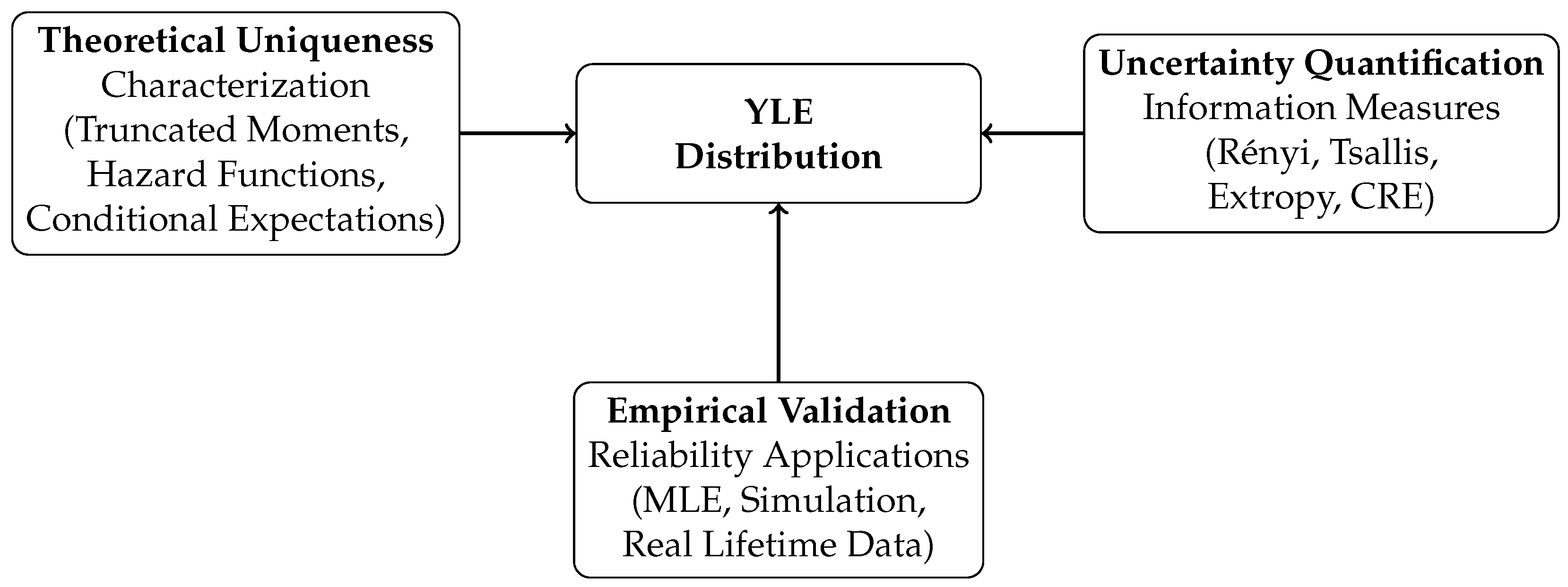
Figure 1 outlines the comprehensive conceptual framework of this study. It illustrates the logical interconnection between the formulation of the YLE distribution, its theoretical validation through mathematical characterizations, its uncertainty quantification via information measures, and its practical implementation in reliability applications, serving as a roadmap for the subsequent sections.

3. Fundamental Properties of the YLE Distribution

In this section, we present the fundamental properties of the YLE distribution to support the next sections on characterizations, information measures, and reliability applications for this distribution.

3.1. Shape Properties of the PDF and HRF of the YLE Distribution

Theorem 1.

Let X follow the YLE distribution with parameters $\alpha \ge 1$, $\lambda \ge 0$, and $\beta \ge 0$. Then:

(i) 

The function $f\left(x\right)$ is decreasing for $\lambda \ge 1$ and $0<\beta \le 1$;

(ii) 

The function $f\left(x\right)$ is unimodal for $0\le \lambda <1$ and $\beta >1$.

Proof. 

Taking the logarithm of the PDF of the YLE distribution, we obtain

$$\begin{array}{cc}\hfill lnf\left(x\right)& =ln\left(4\alpha \right)+ln(\lambda +\beta x)-\lambda x-{\displaystyle \frac{\beta }{2}}{x}^2+(\alpha -1)ln\left[1-{\left(1-e^{-\lambda x-{\displaystyle \frac{\beta }{2}}{x}^2}\right)}^2\right]\hfill \\ \hfill & -2ln\left[{\left(2-e^{-\lambda x-{\displaystyle \frac{\beta }{2}}{x}^2}\right)}^{\alpha }+e^{-\alpha \lambda x-\alpha {\displaystyle \frac{\beta }{2}}{x}^2}\right].\hfill \end{array}$$

(11)

Differentiating with respect to x, we have

$$\begin{array}{cc}\hfill {(lnf\left(x\right))}^{\prime }& ={\displaystyle \frac{\beta }{\lambda +\beta x}}-\lambda -\beta x-{\displaystyle \frac{2(\alpha -1)\left(1-e^{-\lambda x-\frac{\beta }{2}{x}^2}\right)e^{-\lambda x-\frac{\beta }{2}{x}^2}(\lambda +\beta x)}{\left[1-{\left(1-e^{-\lambda x-\frac{\beta }{2}{x}^2}\right)}^2\right]}}\hfill \\ \hfill & -{\displaystyle \frac{2\alpha (\lambda +\beta x)\left[{\left(2-e^{-\lambda x-\frac{\beta }{2}{x}^2}\right)}^{\alpha -1}{e}^{-\lambda x-\frac{\beta }{2}{x}^2}-e^{-\alpha \lambda x-\alpha \frac{\beta }{2}{x}^2}\right]}{\left[{\left(2-e^{-\lambda x-\frac{\beta }{2}{x}^2}\right)}^{\alpha }+e^{-\alpha \lambda x-\alpha \frac{\beta }{2}{x}^2}\right]}}.\hfill \end{array}$$

(12)

• Case (i): For $\lambda \ge 1$ and $0<\beta \le 1$, we have $\beta \le 1<{(1+\beta x)}^2\le {(\lambda +\beta x)}^2$ for all $x>0$, which implies ${\displaystyle \frac{\beta }{\lambda +\beta x}}<\lambda +\beta x$. Since the remaining terms in (12) are products of positive quantities preceded by negative signs, it follows that ${(lnf\left(x\right))}^{\prime }<0$ for all $x>0$. Therefore, $f\left(x\right)$ is decreasing on $(0,\infty )$.
• Case (ii): For $0\le \lambda <1$ and $\beta >1$, in this case $f\left(x\right)$ is unimodal.  

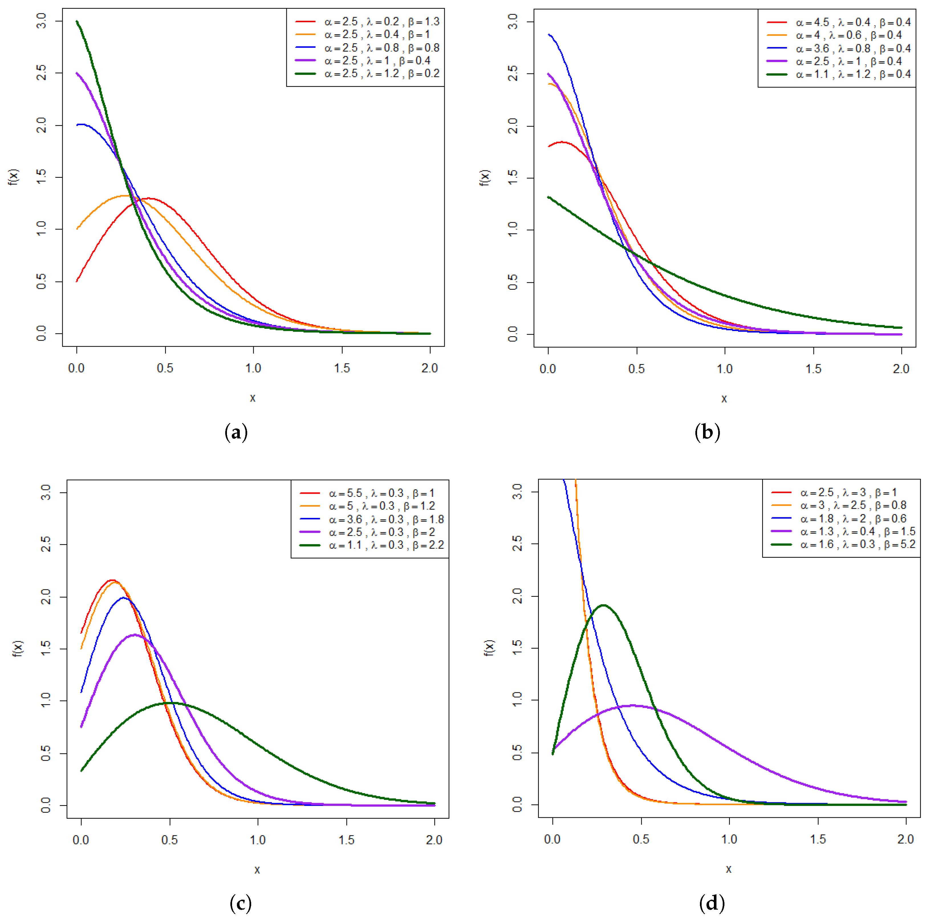
Numerical investigations conducted in R software version 4.5.1 support this behavior. Figure 2 illustrates the shapes of the PDF of the proposed distribution for various parameter combinations, thereby highlighting the flexibility of the YLE distribution in modeling a wide range of right-skewed patterns.

Also note that ${lim}_{x\to \infty }f\left(x\right)=0$ and ${lim}_{x\to 0^{+}}f\left(x\right)=\alpha \lambda$. Consequently, when the density attains its maximum value at $x=0$ (that is, $f\left(0\right)=\alpha \lambda$), the mode is located at $x=0$, resulting in a reversed-J-shaped density, which is consistent with Theorem 1 (Case (i)). On the other hand, when the distribution is unimodal with its peak in $(0,\infty )$, the density function $f\left(x\right)$ possesses at least one interior critical point corresponding to its mode. This interior mode is obtained by solving the equation ${(lnf\left(x\right))}^{\prime }=0$. Thus, we obtain

$$\begin{array}{cc}\hfill {\displaystyle \frac{\beta }{\lambda +\beta x}}& =\lambda +\beta x+{\displaystyle \frac{2(\alpha -1)\left(1-e^{-\lambda x-\frac{\beta }{2}{x}^2}\right)e^{-\lambda x-\frac{\beta }{2}{x}^2}(\lambda +\beta x)}{\left[1-{\left(1-e^{-\lambda x-\frac{\beta }{2}{x}^2}\right)}^2\right]}}\hfill \\ \hfill & +{\displaystyle \frac{2\alpha (\lambda +\beta x)\left[{\left(2-e^{-\lambda x-\frac{\beta }{2}{x}^2}\right)}^{\alpha -1}{e}^{-\lambda x-\frac{\beta }{2}{x}^2}-e^{-\alpha \lambda x-\alpha \frac{\beta }{2}{x}^2}\right]}{\left[{\left(2-e^{-\lambda x-\frac{\beta }{2}{x}^2}\right)}^{\alpha }+e^{-\alpha \lambda x-\alpha \frac{\beta }{2}{x}^2}\right]}}.\hfill \end{array}$$

(13)

Now, if $x=x_0$ is a root, then it is a local maximum if ${\left.{(lnf\left(x\right))}^{\prime \prime }\right|}_{x=x_0}<0,$ a local minimum if ${\left.{(lnf\left(x\right))}^{\prime \prime }\right|}_{x=x_0}>0,$ and a point of inflection if ${\left.{(lnf\left(x\right))}^{\prime \prime }\right|}_{x=x_0}=0.$    □

Likewise, to examine the shape of the hazard-rate function of the YLE distribution, by taking the logarithm of the HRF of the YLE distribution, we obtain

$$\begin{array}{cc}\hfill lnh\left(x\right)& =ln\left(2\alpha \right)+ln(\lambda +\beta x)-\left(\lambda x+{\displaystyle \frac{\beta }{2}}{x}^2\right)+\alpha ln\left(2-e^{-\lambda x-{\displaystyle \frac{\beta }{2}}{x}^2}\right)\hfill \\ \hfill & -ln\left[1-{\left(1-e^{-\lambda x-{\displaystyle \frac{\beta }{2}}{x}^2}\right)}^2\right]-ln\left[{\left(2-e^{-\lambda x-{\displaystyle \frac{\beta }{2}}{x}^2}\right)}^{\alpha }+e^{-\alpha \lambda x-\alpha {\displaystyle \frac{\beta }{2}}{x}^2}\right].\hfill \end{array}$$

(14)

Differentiating with respect to x, we have,

$$\begin{array}{cc}\hfill {(lnh\left(x\right))}^{\prime }& ={\displaystyle \frac{\beta }{\lambda +\beta x}}-\lambda -\beta x+{\displaystyle \frac{\alpha e^{-\lambda x-\frac{\beta }{2}{x}^2}(\lambda +\beta x)}{2-e^{-\lambda x-\frac{\beta }{2}{x}^2}}}+{\displaystyle \frac{2\left(1-e^{-\lambda x-\frac{\beta }{2}{x}^2}\right)e^{-\lambda x-\frac{\beta }{2}{x}^2}(\lambda +\beta x)}{\left[1-{\left(1-e^{-\lambda x-\frac{\beta }{2}{x}^2}\right)}^2\right]}}\hfill \\ \hfill & +{\displaystyle \frac{\alpha (\lambda +\beta x)\left[e^{-\alpha \lambda x-\alpha \frac{\beta }{2}{x}^2}-{\left(2-e^{-\lambda x-\frac{\beta }{2}{x}^2}\right)}^{\alpha -1}{e}^{-\lambda x-\frac{\beta }{2}{x}^2}\right]}{\left[{\left(2-e^{-\lambda x-\frac{\beta }{2}{x}^2}\right)}^{\alpha }+{\left(e^{-\lambda x-\frac{\beta }{2}{x}^2}\right)}^{\alpha }\right]}}.\hfill \end{array}$$

(15)

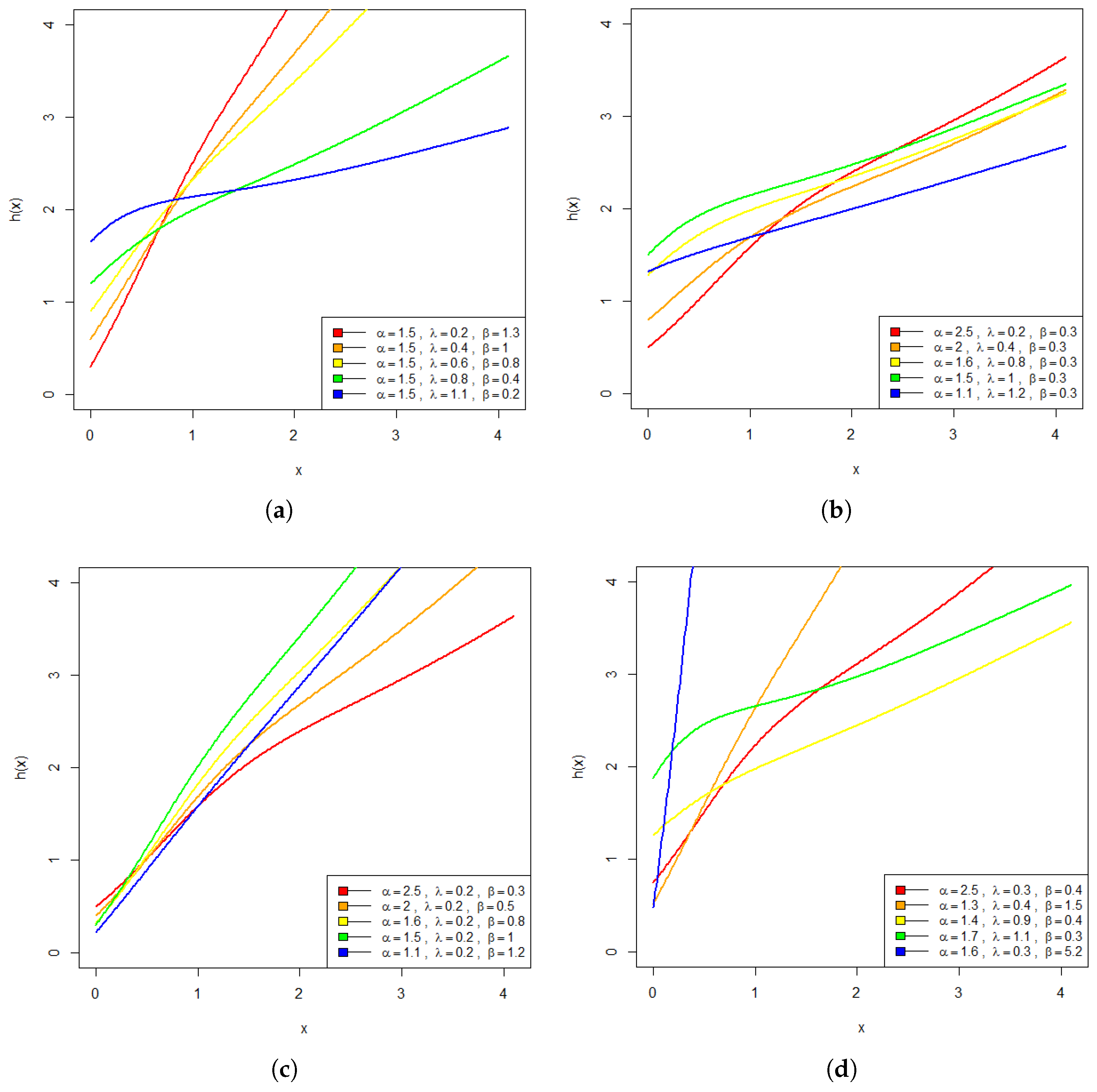
When $\alpha \ge 1$, $\lambda >0$, and $\beta \ge 0$, we observe that ${(lnh\left(x\right))}^{\prime }>0$ for $x>0$, and hence the hazard-rate function $h\left(x\right)$ is increasing. This behavior is supported by numerical evidence obtained using R software version 4.5.1.

The hazard rate plots in Figure 3 illustrate that the YLE distribution exhibits strictly increasing hazard shapes under various parameter settings, demonstrating its ability to model a wide range of increasing hazard patterns commonly observed in reliability and survival data.

3.2. Some Statistical Properties

Statistical properties of the YLE distribution can be deduced from the expression $E\left[Q\right(X\left)\right]$, which is discussed in [20] and has the approximation as follows:

$$\mathrm{E}\left[Q\left(X\right)\right]={\int }_{R}Q\left(x\right)f\left(x\right)dx\approx {\displaystyle \sum _{k,\mathcal{l},m=0}^K}{b}_{k,\mathcal{l},m}{I}_{\mathcal{l},m}(Q,G),$$

(16)

where K is an arbitrary large integer, $b_{k,\mathcal{l},m}=a_k\left(\begin{array}{c}\alpha k\\ \mathcal{l}\end{array}\right)\left(\begin{array}{c}-\alpha k\\ m\end{array}\right){(-1)}^{\mathcal{l}}(\mathcal{l}+m),$ $a_0=1$ and $a_k=2{(-1)}^k$ for $k\ge 1,$ and $I_{\mathcal{l},m}(Q,G)$ can be expressed as  

$$I_{\mathcal{l},m}(Q,G)={\int }_0^{\infty }Q\left(x\right){\left[G\left(x\right)\right]}^{\mathcal{l}+m-1}g\left(x\right)dx.$$

(17)

3.2.1. Ordinary Moments

By substituting $Q\left(x\right)=x^r$ into (16), the rth raw moment of the YLE distribution is given by

$$\mathbb{E}\left[X^r\right]={\int }_0^{\infty }{x}^{r}f\left(x\right)dx\approx {\displaystyle \sum _{k,\mathcal{l},m=0}^K}{b}_{k,\mathcal{l},m}{I}_{\mathcal{l},m}(Q,G).$$

(18)

Using the baseline cumulative distribution function $G\left(x\right)$ and probability density function $g\left(x\right)$ given in (4) and (5), respectively, the functional $I_{\mathcal{l},m}(Q,G)$ defined in (17) can be expressed as

$$\begin{array}{cc}\hfill I_{\mathcal{l},m}(Q,G)& ={\displaystyle \sum _{j=0}^{\mathcal{l}+m-1}}{(-1)}^j\left({\displaystyle \genfrac{}{}{0pt}{}{\mathcal{l}+m-1}{j}}\right){\int }_0^{\infty }{x}^r(\lambda +\beta x)exp\left(-(j+1)\lambda x-{\displaystyle \frac{(j+1)\beta }{2}}{x}^2\right)dx.\hfill \end{array}$$

(19)

Completing the square in the exponent,

$$(j+1)\lambda x+{\displaystyle \frac{(j+1)\beta }{2}}{x}^2={\displaystyle \frac{(j+1)\beta }{2}}{\left(x+{\displaystyle \frac{\lambda }{\beta }}\right)}^2-{\displaystyle \frac{(j+1){\lambda }^2}{2\beta }},$$

and introducing the transformation

$$y=\sqrt{(j+1)\beta }\left(x+{\displaystyle \frac{\lambda }{\beta }}\right),a_j={\displaystyle \frac{(j+1)\lambda }{\sqrt{(j+1)\beta }}},$$

the integrals reduce to moments of a truncated normal distribution. Then $I_{\mathcal{l},m}(Q,G)$ becomes

$$I_{\mathcal{l},m}(Q,G)={\displaystyle \sum _{j=0}^{\mathcal{l}+m-1}}{(-1)}^j\left({\displaystyle \genfrac{}{}{0pt}{}{\mathcal{l}+m-1}{j}}\right)C_j\left[\lambda M_r\left(a_j\right)+\beta M_{r+1}\left(a_j\right)\right],$$

(20)

where

$$C_j=exp\left({\displaystyle \frac{(j+1){\lambda }^2}{2\beta }}\right){\left({\displaystyle \frac{2\pi }{(j+1)\beta }}\right)}^{1/2},$$

$$M_q\left(a_j\right)={\int }_{a_j}^{\infty }{\left({\displaystyle \frac{y}{\sqrt{(j+1)\beta }}}-{\displaystyle \frac{\lambda }{\beta }}\right)}^q\varphi \left(y\right)dy,q\ge 0,$$

and $\varphi \left(y\right)={\left(2\pi \right)}^{-1/2}exp(-y^2/2)$ denotes the standard normal density. The quantities $M_q\left(a_j\right)$ have closed-form expressions in terms of the standard normal cumulative distribution function or the error function. This formulation provides a numerically stable and analytically tractable representation for the ordinary moments of the YLE distribution.

From the raw moments, the mean, variance, skewness, and kurtosis for the YLE distribution can be derived. Table 1 summarizes the moment characteristics of the YLE distribution for various parameter values. The results show that both the mean and variance decrease as $\alpha$, $\lambda$, and $\beta$ increase. Skewness remains positive for all cases and increases with the parameters, confirming a consistently right-skewed structure. Similarly, kurtosis values exceed 3 across all configurations and grow with parameter magnitude, demonstrating increasingly peaked and heavy-tailed shapes. These findings suggest that the YLE distribution is flexible and well-suited for modeling right-skewed, heavy-tailed data.

3.2.2. Moment Generating Function

By substituting $Q\left(x\right)=e^{tx}$ into (16), the moment generating function is given as

$$\mathrm{E}\left[e^{tx}\right]={\int }_0^{\infty }{e}^{tx}f\left(x\right)dx\approx {\displaystyle \sum _{k,\mathcal{l},m=0}^K}{b}_{k,\mathcal{l},m}{I}_{\mathcal{l},m}(Q,G).$$

(21)

Using the baseline cumulative distribution function $G\left(x\right)$ and probability density function $g\left(x\right)$ given in (4) and (5), respectively, the functional $I_{\mathcal{l},m}(Q,G)$ defined in (17) can be expressed as

$$\begin{array}{cc}\hfill I_{\mathcal{l},m}(e^{tx},G)& ={\displaystyle \sum _{j=0}^{\mathcal{l}+m-1}}{(-1)}^j\left({\displaystyle \genfrac{}{}{0pt}{}{\mathcal{l}+m-1}{j}}\right){\int }_0^{\infty }(\lambda +\beta x)exp\left(-A_j\left(t\right)x-{\displaystyle \frac{(j+1)\beta }{2}}{x}^2\right)dx,\hfill \end{array}$$

(22)

where

$$A_j\left(t\right)=(j+1)\lambda -t.$$

Completing the square in the exponent,

$$A_j\left(t\right)x+{\displaystyle \frac{(j+1)\beta }{2}}{x}^2={\displaystyle \frac{(j+1)\beta }{2}}{\left(x+{\displaystyle \frac{A_j\left(t\right)}{(j+1)\beta }}\right)}^2-{\displaystyle \frac{A_j{\left(t\right)}^2}{2(j+1)\beta }},$$

and introducing the transformation

$$y=\sqrt{(j+1)\beta }\left(x+{\displaystyle \frac{A_j\left(t\right)}{(j+1)\beta }}\right),a_j\left(t\right)={\displaystyle \frac{A_j\left(t\right)}{\sqrt{(j+1)\beta }}},$$

the integrals reduce to truncated normal integrals. Then $I_{\mathcal{l},m}(e^{tx},G)$ becomes

$$I_{\mathcal{l},m}(e^{tx},G)={\displaystyle \sum _{j=0}^{\mathcal{l}+m-1}}{(-1)}^j\left({\displaystyle \genfrac{}{}{0pt}{}{\mathcal{l}+m-1}{j}}\right)C_j\left(t\right)\left[\lambda {\tilde{M}}_0\left(a_j\left(t\right)\right)+\beta {\tilde{M}}_1\left(a_j\left(t\right)\right)\right],$$

(23)

where

$$C_j\left(t\right)=exp\left({\displaystyle \frac{A_j{\left(t\right)}^2}{2(j+1)\beta }}\right){\left({\displaystyle \frac{2\pi }{(j+1)\beta }}\right)}^{1/2},$$

and

$${\tilde{M}}_q\left(a\right)={\int }_a^{\infty }{y}^q\varphi \left(y\right)dy,q\ge 0,$$

with $\varphi \left(y\right)={\left(2\pi \right)}^{-1/2}exp(-y^2/2)$ denoting the standard normal density.

3.2.3. Quantile Function

The quantile function is crucial for simulation and calculating quantile-based measures. The quantile function of the Yun-G family is given in (7), for the YLE distribution, the quantile function $G^{-1}\left(y\right)$ is obtained by solving

$$y=1-e^{-\lambda q-{\displaystyle \frac{\beta }{2}}{q}^2}\Rightarrow e^{-\lambda q-{\displaystyle \frac{\beta }{2}}{q}^2}=1-y.$$

Taking the natural logarithm

$$-\lambda q-{\displaystyle \frac{\beta }{2}}{q}^2=ln(1-y).$$

$${\displaystyle \frac{\beta }{2}}{q}^2+\lambda q+ln(1-y)=0.$$

This is a quadratic equation in q. Using the quadratic formula and choosing the positive root (since $q\ge 0$), we obtain

$$G^{-1}\left(y\right)=q={\displaystyle \frac{-\lambda +\sqrt{{\lambda }^2-2\beta ln(1-y)}}{\beta }},\mathrm{for}\beta >0.$$

If $\beta =0$, the linear exponential reduces to the exponential distribution, and

$$G^{-1}\left(y\right)=-{\displaystyle \frac{ln(1-y)}{\lambda }}.$$

Therefore, the quantile function of the YLE distribution is

$$Q\left(u\right)={\displaystyle \frac{-\lambda +\sqrt{{\lambda }^2-2\beta ln\left[1-T_{1/\alpha }\left(u\right)\right]}}{\beta }},\beta >0,$$

(24)

where

$$T_{1/\alpha }\left(u\right)={\displaystyle \frac{{(1+u)}^{1/\alpha }-{(1-u)}^{1/\alpha }}{{(1+u)}^{1/\alpha }+{(1-u)}^{1/\alpha }}},u\in [0,1].$$

To study the limiting behavior of the quantile function in (24), we examine the limit as $\beta \to 0$. Since both the numerator and denominator tend to zero, the expression is of the indeterminate form $0/0$.

Applying L’Hôpital’s rule, we obtain

$$\underset{\beta \to 0}{lim}Q\left(u\right)=-\underset{\beta \to 0}{lim}\left[{\displaystyle \frac{ln\left(1-T_{1/\alpha }\left(u\right)\right)}{\sqrt{{\lambda }^2-2\beta ln\left(1-T_{1/\alpha }\left(u\right)\right)}}}\right]=-{\displaystyle \frac{1}{\lambda }}ln\left(1-T_{1/\alpha }\left(u\right)\right).$$

Thus, the quantile function of the YLE distribution converges to that of the Yun–Exponential distribution as $\beta \to 0$.

4. Characterizations of YLE Distribution

Characterization results play an important role in probability theory and statistical modeling because they provide alternative criteria for uniquely identifying a probability distribution. In addition to establishing the uniqueness of the proposed YLE distribution, the characterizations developed in this section offer different perspectives on its probabilistic structure. The characterization based on truncated moments extends the well-established framework developed [1,2] and identifies the proposed distribution through specific relationships between truncated moments. Besides providing a rigorous characterization criterion, such results may also serve as a basis for parameter estimation and further theoretical developments. The hazard function and reversed hazard function characterizations connect the YLE distribution to reliability and survival analysis, where failure-rate functions are of primary interest. Furthermore, the characterization based on conditional expectations provides an alternative stochastic representation of the model and offers additional insight into its underlying probabilistic structure. In particular, the characterization results derived through multiple mathematical frameworks demonstrate that the proposed model is not only flexible but also rigorously identifiable through several independent mathematical structures. Collectively, these results strengthen the theoretical foundation of the YLE distribution, provide complementary insights into its underlying probabilistic behavior, and enhance its applicability in reliability analysis and stochastic modeling.

4.1. Characterization Based on Truncated Moments

This subsection focuses on characterization results for the YLE distribution derived from the ratio of two truncated moments. The results are obtained by applying Theorem of [1].

Proposition 1.

Let $(\Omega ,\mathcal{F},\mathbb{P})$ be a given probability space, and let $H=[a,b]$ be an interval for some $a<b$ (where $a=-\infty$ or $b=\infty$ might as well be allowed). Let $X:\Omega \to H$ be a continuous random variable with distribution function $F\left(x\right)$ and let $q_1$ and $q_2$ be two real functions defined on H such that

$$\mathbb{E}\left[q_1\left(X\right)\mid X\ge x\right]=\mathbb{E}\left[q_2\left(X\right)\mid X\ge x\right]\psi \left(x\right),x\in H,$$

is defined with some real function ψ. Assume that $q_1,q_2\in C^1\left(H\right)$, $\psi \in C^2\left(H\right)$, and that $F\left(x\right)$ is a twice continuously differentiable and strictly monotone function on the set H. Finally, assume that the equation $\psi q_1=q_2$ has no real solution in the interior of H. Then F is uniquely determined by the functions $q_1$, $q_2$, and ψ, particularly

$$F\left(x\right)={\int }_a^{x}K\left|{\displaystyle \frac{{\psi }^{\prime }\left(u\right)}{\psi \left(u\right)q_1\left(u\right)-q_2\left(u\right)}}\right|e^{-s\left(u\right)}du,$$

where the function s is a solution of the differential equation $s^{\prime }={\displaystyle \frac{{\psi }^{\prime }{q}_1}{\psi q_1-q_2}}$, and K is the normalization constant, such that ${\int }_{H}dF=1$.

Please note that the result, however, also holds when the interval H is not closed, since the condition is on the interior of H.

Theorem 2.

Let $X:\Omega \to (0,\infty )$ be a continuous random variable, and let $q_1\left(x\right)={\left[(2-e^{-\lambda x-{\displaystyle \frac{\beta }{2}}{x}^2}{)}^{\alpha }+(e^{-\alpha \lambda x-\alpha {\displaystyle \frac{\beta }{2}}{x}^2})\right]}^2(2-e^{-\lambda x-{\displaystyle \frac{\beta }{2}}{x}^2}{)}^{1-\alpha }$ and $q_2\left(x\right)=q_1\left(x\right)e^{-\alpha \lambda x-\alpha {\displaystyle \frac{\beta }{2}}{x}^2}$ for $x>0$. The PDF of X is given by (9) if and only if the function ψ defined in Proposition 1 has the form

$$\psi \left(x\right)={\displaystyle \frac{1}{2}}{e}^{-\alpha \lambda x-\alpha {\displaystyle \frac{\beta }{2}}{x}^2},x>0.$$

(25)

Proof. 

Let X have PDF in (9), then

$$(1-F\left(x\right))\mathbb{E}[q_1\left(X\right)\mid X\ge x]=4e^{-\alpha \lambda x-\alpha {\displaystyle \frac{\beta }{2}}{x}^2},x>0,$$

$$(1-F\left(x\right))\mathbb{E}[q_2\left(X\right)\mid X\ge x]=2e^{2(-\alpha \lambda x-\alpha {\displaystyle \frac{\beta }{2}}{x}^2)},x>0,$$

and then

$$\psi \left(x\right)q_1\left(x\right)-q_2\left(x\right)=-{\displaystyle \frac{1}{2}}{q}_1\left(x\right)e^{-\alpha \lambda x-\alpha {\displaystyle \frac{\beta }{2}}{x}^2}<0,\mathrm{for}x>0.$$

(26)

Conversely, if $\psi$ is given as (25), then

$$s^{\prime }\left(x\right)={\displaystyle \frac{{\psi }^{\prime }\left(x\right)q_1\left(x\right)}{\psi \left(x\right)q_1\left(x\right)-q_2\left(x\right)}}=\alpha (\lambda +\beta x),x>0.$$

(27)

and hence

$$s\left(x\right)=\alpha \lambda x+\alpha {\displaystyle \frac{\beta }{2}}{x}^2,x>0,$$

or

$$e^{-s\left(x\right)}=e^{-\alpha \lambda x-\alpha {\displaystyle \frac{\beta }{2}}{x}^2},x>0.$$

Now, in view of Proposition 1, X has density (9).    □

Corollary 1.

Let $X:\Omega \to (0,\infty )$ be a continuous random variable and let $q_1\left(x\right)$ be as in Theorem 2. The PDF of X is given by (9) if and only if there exist functions $q_2$ and ψ defined in Proposition 1 satisfying the differential equation

$${\displaystyle \frac{{\psi }^{\prime }\left(x\right)q_1\left(x\right)}{\psi \left(x\right)q_1\left(x\right)-q_2\left(x\right)}}=\alpha (\lambda +\beta x),x>0.$$

(28)

The general solution of the differential equation given in Corollary 1 is

$$\psi \left(x\right)=e^{\alpha \lambda x+\alpha {\displaystyle \frac{\beta }{2}}{x}^2}\left[-\int \alpha (\lambda +\beta x)e^{-\alpha \lambda x-\alpha {\displaystyle \frac{\beta }{2}}{x}^2}{\left(q_1\left(x\right)\right)}^{-1}{q}_2\left(x\right)dx+D\right],$$

(29)

where D is a constant.

4.2. Characterization Based on Hazard Function

Let $X:(0,\infty )\to \mathbb{R}$ be a continuous random variable with PDF $f\left(x\right)$ and hazard-rate function $h\left(x\right)$. A useful characterization of the density function in terms of the hazard-rate function is given by

$${\displaystyle \frac{f^{\prime }\left(x\right)}{f\left(x\right)}}={\displaystyle \frac{h^{\prime }\left(x\right)}{h\left(x\right)}}-h\left(x\right),x>0.$$

(30)

Theorem 3.

Let $X:\Omega \to (0,+\infty )$ has a YLE $(\alpha ,\lambda ,\beta )$ if and only if the HRF $h\left(x\right)$, defined by (10), satisfies the following equation

$${\displaystyle \frac{h^{\prime }\left(x\right)}{{\left(h\left(x\right)\right)}^2}}={\displaystyle \frac{{(2-z)}^{\alpha }+z^{\alpha }}{2\alpha (\lambda +\beta x){(2-z)}^{\alpha -1}}}\left[{\displaystyle \frac{\beta }{\lambda +\beta x}}+(\alpha -1){\displaystyle \frac{(\lambda +\beta x)z}{2-z}}-{\displaystyle \frac{\alpha (\lambda +\beta x)\left({(2-z)}^{\alpha -1}z-z^{\alpha }\right)}{{(2-z)}^{\alpha }+z^{\alpha }}}\right],$$

(31)

where $z=exp\left(-\lambda x-{\displaystyle \frac{\beta }{2}}{x}^2\right)$.

Proof. 

Let $X\sim \mathrm{YLE}$$(\alpha ,\lambda ,\beta )$, where the PDF $f\left(x\right)$ is defined in (9). Then, the logarithm of $f\left(x\right)$ can be expressed as

$$lnf\left(x\right)=ln\left(4\alpha \right)+ln(\lambda +\beta x)-\alpha \lambda x-\alpha {\displaystyle \frac{\beta }{2}}{x}^2+(\alpha -1)ln(2-z)-2ln\left[{(2-z)}^{\alpha }+z^{\alpha }\right].$$

(32)

Differentiating both sides of the above equation with respect to x yields

$${\displaystyle \frac{d}{dx}}lnf\left(x\right)={\displaystyle \frac{\beta }{\lambda +\beta x}}-\alpha \lambda -\alpha \beta x+(\alpha -1){\displaystyle \frac{(\lambda +\beta x)z}{2-z}}-{\displaystyle \frac{2\alpha (\lambda +\beta x)\left[{(2-z)}^{\alpha -1}z-z^{\alpha }\right]}{{(2-z)}^{\alpha }+z^{\alpha }}}.$$

(33)

Thus, according to (10) and (30), it follows that

$$\begin{array}{cc}\hfill {\displaystyle \frac{d}{dx}}lnf\left(x\right)+h\left(x\right)& ={\displaystyle \frac{\beta }{\lambda +\beta x}}-\alpha \lambda -\alpha \beta x+(\alpha -1){\displaystyle \frac{(\lambda +\beta x)z}{2-z}}\hfill \\ \hfill & +{\displaystyle \frac{2\alpha (\lambda +\beta x)\left[{(2-z)}^{\alpha -1}(1-z)+z^{\alpha }\right]}{{(2-z)}^{\alpha }+z^{\alpha }}},\hfill \end{array}$$

(34)

which, after appropriate simplifications, leads to (31).

Suppose that (31) holds. Integrating both sides, we obtain

$$\begin{array}{cc}\hfill \int {\displaystyle \frac{h^{\prime }\left(x\right)}{{\left(h\left(x\right)\right)}^2}}dx& =\int {\displaystyle \frac{{(2-z)}^{\alpha }+z^{\alpha }}{2\alpha (\lambda +\beta x){(2-z)}^{\alpha -1}}}\hfill \\ \hfill & \times \left[{\displaystyle \frac{\beta }{\lambda +\beta x}}+(\alpha -1){\displaystyle \frac{(\lambda +\beta x)z}{2-z}}-{\displaystyle \frac{\alpha (\lambda +\beta x)\left({(2-z)}^{\alpha -1}z-z^{\alpha }\right)}{{(2-z)}^{\alpha }+z^{\alpha }}}\right]dx.\hfill \end{array}$$

(35)

That is, we have

$$-{\displaystyle \frac{1}{h\left(x\right)}}=-{\displaystyle \frac{{(2-z)}^{\alpha }+z^{\alpha }}{2\alpha (\lambda +\beta x){(2-z)}^{\alpha -1}}}.$$

(36)

From (36), we obtain the HRF as shown in (10). Furthermore, by replacing this function in (30), and after integration, we obtain

$$\begin{array}{cc}\hfill lnf\left(x\right)& =\int [{\displaystyle \frac{\beta }{\lambda +\beta x}}-\alpha \lambda -\alpha \beta x+(\alpha -1){\displaystyle \frac{(\lambda +\beta x)z}{2-z}}\hfill \\ \hfill & -{\displaystyle \frac{2\alpha (\lambda +\beta x)\left({(2-z)}^{\alpha -1}z-z^{\alpha }\right)}{{(2-z)}^{\alpha }+z^{\alpha }}}]dx+C_1\hfill \\ \hfill & =ln(\lambda +\beta x)-\alpha \lambda x-\alpha {\displaystyle \frac{\beta }{2}}{x}^2+(\alpha -1)ln(2-z)\hfill \\ \hfill & -2ln\left[{(2-z)}^{\alpha }+z^{\alpha }\right]+C_1.\hfill \end{array}$$

(37)

That is, we have

$$f\left(x\right)=(\lambda +\beta x)e^{C_1}{z}^{\alpha }{(2-z)}^{\alpha -1}{\left[{(2-z)}^{\alpha }+z^{\alpha }\right]}^{-2},$$

(38)

and

$$F\left(x\right)={\displaystyle \frac{e^{C_1}\left({(2-z)}^{\alpha }-z^{\alpha }\right)}{4\alpha \left({(2-z)}^{\alpha }+z^{\alpha }\right)}}+C_2,$$

(39)

whereby from the conditions $F\left(0\right)=0$ and $F(\infty )=1$, the constants $e^{C_1}=4\alpha$ and $C_2=0$ are obtained. Thus, the function $F\left(x\right)$ is indeed the CDF from the YLE distribution, which completes the proof.    □

Practical Application of the Hazard Characterization

While characterization theorems are predominantly utilized as theoretical validations of a probability model, they can also be implemented as powerful diagnostic tools in applied data analysis. Based on Theorem 3, a continuous random variable X follows the YLE distribution if and only if the ratio $\eta \left(x\right)={\displaystyle \frac{h^{\prime }\left(x\right)}{{\left(h\left(x\right)\right)}^2}}$, is equal to the right-hand side of (31), which we can denote as $\Psi (x;\alpha ,\lambda ,\beta )$. This strict mathematical identity offers a novel graphical diagnostic method for assessing goodness-of-fit. For a given lifetime dataset, one can estimate the empirical hazard rate $\widehat{h}\left(x\right)$ using non-parametric kernel smoothing techniques. In this study, we employed the kernel hazard estimator implemented in the muhaz package in R, using a global bandwidth selection procedure with boundary correction at both ends of the support. To obtain a stable estimate of the derivative, the estimated hazard function was subsequently smoothed using a cubic smoothing spline, and the derivative was computed directly from the fitted spline. The empirical characterization ratio was then calculated as $\widehat{\eta }\left(x\right)={\displaystyle \frac{{\widehat{h}}^{\prime }\left(x\right)}{\widehat{h}{\left(x\right)}^2}}$. By plotting $\widehat{\eta }\left(x\right)$ alongside the theoretical curve $\Psi (x;\widehat{\alpha },\widehat{\lambda },\widehat{\beta })$, evaluated using the maximum-likelihood estimates of the parameters, one can visually assess the agreement between the two curves. A strong convergence between the empirical and theoretical curves not only serves as an alternative goodness-of-fit diagnostic but also provides direct empirical validation of the characterization theorem established in (31).

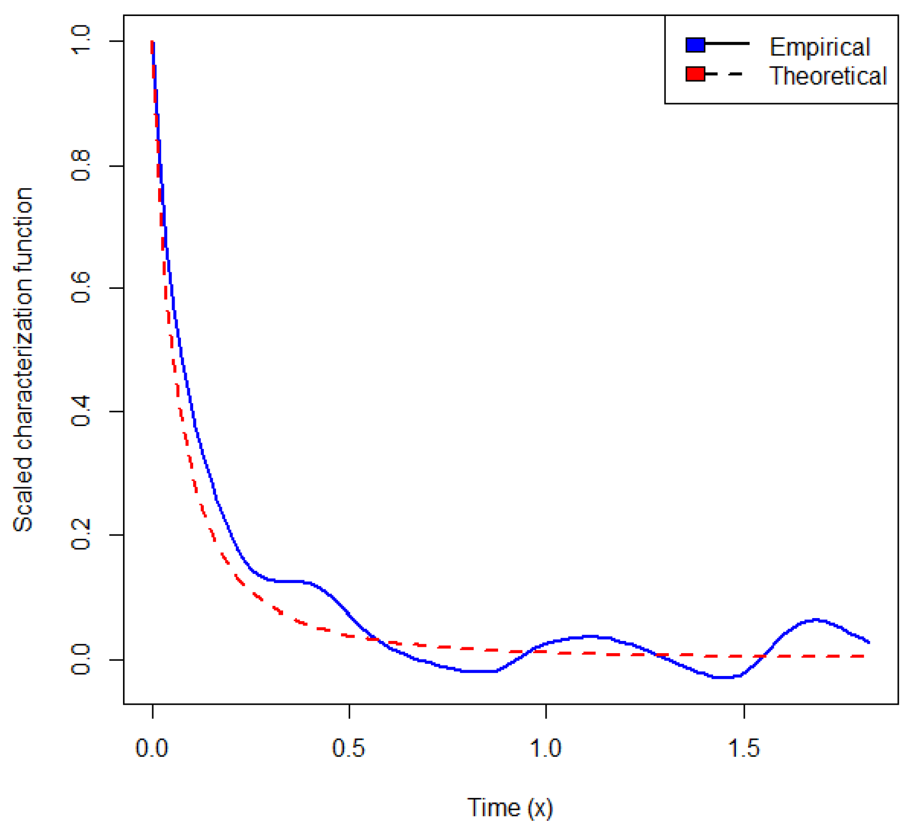
In this study, we utilize the second dataset presented in Section 8. The corresponding diagnostic plot is shown in Figure 4. To facilitate comparison, both the empirical and theoretical characterization functions are scaled to a common range. The resulting plot demonstrates a strong agreement in the overall decreasing trend of the two curves, particularly in the lower and moderate ranges of x. The empirical curve closely follows the theoretical function in the initial region, indicating consistency with the proposed characterization. Although minor oscillations are observed in the empirical curve for larger values of x, these deviations can be attributed to numerical sensitivity in estimating the derivative of the hazard function and the limited sample size.

To complement the graphical assessment, a quantitative comparison was also performed between the empirical and theoretical characterization functions. Specifically, the root mean square error (RMSE) and the Pearson correlation coefficient were computed using the scaled characterization functions. The resulting RMSE was 0.0415, while the correlation coefficient was 0.9793, indicating a very close agreement between the empirical and theoretical curves.

To assess the robustness of the diagnostic procedure, a sensitivity analysis was conducted by varying the smoothing parameter (spar) of the cubic smoothing spline. In addition to the reference value (spar = 0.6) used for the main analysis, alternative values of spar = 0.5, spar = 0.7, and spar = 0.8 were also examined. The resulting empirical characterization curves exhibited similar overall behavior across all smoothing levels, with only minor differences in local fluctuations.

Overall, the observed agreement between the empirical and theoretical curves provides supporting evidence for the validity of the hazard-based characterization of the YLE distribution.

4.3. Characterization in Terms of the Reversed Hazard Function

Theorem 4.

Let $X:\Omega \to (0,\infty )$ be a continuous random variable. The PDF of X is given by (9) if and only if its reversed hazard-rate function $r\left(x\right)$ satisfies

$$r^{\prime }\left(x\right)+{\displaystyle \frac{D^{\prime }\left(x\right)}{D\left(x\right)}}r\left(x\right)=H\left(x\right),x>0,$$

(40)

where

$$D\left(x\right)={\left(2-e^{-\lambda x-{\displaystyle \frac{\beta }{2}}{x}^2}\right)}^{2\alpha }-e^{-2\alpha \lambda x-\alpha \beta x^2},$$

and

$$H\left(x\right)={\displaystyle \frac{4\alpha e^{-\alpha \lambda x-\alpha \frac{\beta }{2}{x}^2}}{D\left(x\right)}}[\beta {\left(2-e^{-\lambda x-{\displaystyle \frac{\beta }{2}}{x}^2}\right)}^{\alpha -1}-\alpha {(\lambda +\beta x)}^2{\left(2-e^{-\lambda x-{\displaystyle \frac{\beta }{2}}{x}^2}\right)}^{\alpha -1}$$

$$+(\alpha -1){(\lambda +\beta x)}^2{e}^{-\lambda x-{\displaystyle \frac{\beta }{2}}{x}^2}{\left(2-e^{-\lambda x-{\displaystyle \frac{\beta }{2}}{x}^2}\right)}^{\alpha -2}],$$

with boundary condition ${lim}_{x\to 0}r\left(x\right)=0$.

Proof. 

If X has PDF given by (9), then its reversed hazard-rate function is

$$r\left(x\right)={\displaystyle \frac{f\left(x\right)}{F\left(x\right)}}.$$

Substituting the expressions of $f\left(x\right)$ and $F\left(x\right)$, we obtain

$$r\left(x\right)={\displaystyle \frac{4\alpha (\lambda +\beta x)e^{-\alpha \lambda x-\alpha \frac{\beta }{2}{x}^2}{\left(2-e^{-\lambda x-\frac{\beta }{2}{x}^2}\right)}^{\alpha -1}}{D\left(x\right)}}.$$

(41)

Differentiating $r\left(x\right)$ using logarithmic differentiation, we obtain

$${\displaystyle \frac{r^{\prime }\left(x\right)}{r\left(x\right)}}={\displaystyle \frac{d}{dx}}lnr\left(x\right)={\displaystyle \frac{d}{dx}}\left[ln(\lambda +\beta x)-\alpha \lambda x-\alpha {\displaystyle \frac{\beta }{2}}{x}^2+(\alpha -1)ln\left(2-e^{-\lambda x-{\displaystyle \frac{\beta }{2}}{x}^2}\right)-lnD\left(x\right)\right].$$

On simplification, this yields

$$r^{\prime }\left(x\right)+{\displaystyle \frac{D^{\prime }\left(x\right)}{D\left(x\right)}}r\left(x\right)=H\left(x\right),$$

which proves that the given differential equation holds.

Conversely, assume that the reversed hazard-rate function $r\left(x\right)$ satisfies

$$r^{\prime }\left(x\right)+P\left(x\right)r\left(x\right)=H\left(x\right),$$

(42)

where $P\left(x\right)={\displaystyle \frac{D^{\prime }\left(x\right)}{D\left(x\right)}}$.

The solution of the above differential equation is given by $r\left(x\right)={\displaystyle \frac{1}{u\left(x\right)}}\left[\int u\left(x\right)H\left(x\right)dx+C\right],$ where $u\left(x\right)=e^{\int P\left(x\right)dx}$ is the integrating factor. Here, $u\left(x\right)=e^{\int {\displaystyle \frac{D^{\prime }\left(x\right)}{D\left(x\right)}}dx}=D\left(x\right).$

Thus, the solution becomes

$$r\left(x\right)={\displaystyle \frac{1}{D\left(x\right)}}\left[\int D\left(x\right)H\left(x\right)dx+C\right].$$

(43)

Next, observe that

$$D\left(x\right)H\left(x\right)=4\alpha e^{-\alpha \lambda x-\alpha {\displaystyle \frac{\beta }{2}}{x}^2}[\beta {(2-e^{-\lambda x-{\displaystyle \frac{\beta }{2}}{x}^2})}^{\alpha -1}-\alpha {(\lambda +\beta x)}^2{(2-e^{-\lambda x-{\displaystyle \frac{\beta }{2}}{x}^2})}^{\alpha -1}$$

(44)

$$+(\alpha -1){(\lambda +\beta x)}^2{e}^{-\lambda x-{\displaystyle \frac{\beta }{2}}{x}^2}{(2-e^{-\lambda x-{\displaystyle \frac{\beta }{2}}{x}^2})}^{\alpha -2}].$$

Also note that

$$D\left(x\right)H\left(x\right)={\displaystyle \frac{d}{dx}}\left[4\alpha (\lambda +\beta x)e^{-\alpha \lambda x-\alpha {\displaystyle \frac{\beta }{2}}{x}^2}{(2-e^{-\lambda x-{\displaystyle \frac{\beta }{2}}{x}^2})}^{\alpha -1}\right].$$

(45)

Hence,

$$\int D\left(x\right)H\left(x\right)dx=4\alpha (\lambda +\beta x)e^{-\alpha \lambda x-\alpha {\displaystyle \frac{\beta }{2}}{x}^2}{(2-e^{-\lambda x-{\displaystyle \frac{\beta }{2}}{x}^2})}^{\alpha -1}.$$

(46)

Substituting back in (43), and using the boundary condition ${lim}_{x\to 0}r\left(x\right)=0$, we find that $C=0$ is necessary to ensure the regularity of the reversed hazard rate at the origin. Thus, we obtain

$$r\left(x\right)={\displaystyle \frac{4\alpha (\lambda +\beta x)e^{-\alpha \lambda x-\alpha \frac{\beta }{2}{x}^2}{(2-e^{-\lambda x-\frac{\beta }{2}{x}^2})}^{\alpha -1}}{D\left(x\right)}},$$

which is the reversed hazard-rate function of the YLE distribution. This completes the proof. □

4.4. Characterization Based on the Conditional Expectation of a Certain Function of the Random Variable

Theorem 5.

Let $X:\Omega \to (0,\infty )$ be a continuous random variable with CDF $F\left(x\right)$. Let $\psi \left(x\right)$ be a differentiable function on $(0,\infty )$ such that

$$\psi \left(x\right)=\delta {\left[1-{\left({\displaystyle \frac{(2-e^{-\lambda x-\frac{\beta }{2}{x}^2}{)}^{\alpha }-e^{-\alpha \lambda x-\alpha \frac{\beta }{2}{x}^2}}{(2-e^{-\lambda x-\frac{\beta }{2}{x}^2}{)}^{\alpha }+e^{-\alpha \lambda x-\alpha \frac{\beta }{2}{x}^2}}}\right)}^{{\displaystyle \frac{1}{\delta -1}}}\right]}^{-1},$$

(47)

where $\delta >1$.

Then $E\left[{\left(\psi \left(X\right)\right)}^{\delta }|X\le x\right]=\delta {\left(\psi \left(x\right)\right)}^{\delta -1}$ for $x\in (0,\infty )$, if and only if $X\sim {\displaystyle YLE}$$(\alpha ,\lambda ,\beta )$ distribution.

Proof. 

If $X\sim \mathrm{YLE}$$(\alpha ,\lambda ,\beta )$, then $E\left[{\left(\psi \left(X\right)\right)}^{\delta }|X\le x\right]=\delta {\left(\psi \left(x\right)\right)}^{\delta -1}$ implies

$${\int }_0^x{\left(\psi \left(u\right)\right)}^{\delta }f\left(u\right)du=\delta {\left(\psi \left(x\right)\right)}^{\delta -1}F\left(x\right).$$

(48)

Taking derivatives on both sides of the above equation with respect to x, we obtain

$${\left(\psi \left(x\right)\right)}^{\delta }f\left(x\right)=\delta \left[(\delta -1){\psi }^{\prime }\left(x\right){\left(\psi \left(x\right)\right)}^{\delta -2}F\left(x\right)+{\left(\psi \left(x\right)\right)}^{\delta -1}f\left(x\right)\right].$$

(49)

Rearranging the terms, we have

$${\displaystyle \frac{f\left(x\right)}{F\left(x\right)}}=\delta (\delta -1){\displaystyle \frac{{\psi }^{\prime }\left(x\right)}{\psi \left(x\right)\left(\psi \right(x)-\delta )}}.$$

(50)

Using partial fraction expansion, the equation becomes

$${\displaystyle \frac{f\left(x\right)}{F\left(x\right)}}=(\delta -1)\left[-{\displaystyle \frac{{\psi }^{\prime }\left(x\right)}{\psi \left(x\right)}}+{\displaystyle \frac{{\psi }^{\prime }\left(x\right)}{\psi \left(x\right)-\delta }}\right].$$

(51)

Integrating both sides of the above equation and applying the limit $x\to \infty$, we obtain

$$F\left(x\right)={\left[1-{\displaystyle \frac{\delta }{\psi \left(x\right)}}\right]}^{\delta -1}.$$

(52)

Substituting the expression for $\psi \left(x\right)$ given in (47) into (52), we obtain

$$F\left(x\right)={\displaystyle \frac{{(2-e^{-\lambda x-\frac{\beta }{2}{x}^2})}^{\alpha }-e^{-\alpha \lambda x-\alpha \frac{\beta }{2}{x}^2}}{{(2-e^{-\lambda x-\frac{\beta }{2}{x}^2})}^{\alpha }+e^{-\alpha \lambda x-\alpha \frac{\beta }{2}{x}^2}}}.$$

(53)

That is, X follows the YLE distribution. □

Theorem 6.

Let $X:\Omega \to (0,\infty )$ be a continuous random variable with CDF $F\left(x\right)$ and survival function $\overline{F}\left(x\right)=1-F\left(x\right)$. Let $\varphi \left(x\right)$ be a differentiable function on $(0,\infty )$ defined as

$$\varphi \left(x\right)=\delta {\left[1+{\left({\displaystyle \frac{2e^{-\alpha (\lambda x+\frac{\beta }{2}{x}^2)}}{(2-e^{-\lambda x-\frac{\beta }{2}{x}^2}{)}^{\alpha }+e^{-\alpha \lambda x-\alpha \frac{\beta }{2}{x}^2}}}\right)}^{{\displaystyle \frac{1}{\delta -1}}}\right]}^{-1},$$

(54)

where $\delta >1$.

Then $E\left[{\left(\varphi \left(X\right)\right)}^{\delta }|X\ge x\right]=\delta {\left(\varphi \left(x\right)\right)}^{\delta -1}$ for $x\in (0,\infty )$, if and only if $X\sim {\displaystyle YLE}$$(\alpha ,\lambda ,\beta )$ distribution.

Proof. 

If $X\sim \mathrm{YLE}$$(\alpha ,\lambda ,\beta )$, the identity $E\left[{\left(\varphi \left(X\right)\right)}^{\delta }|X\ge x\right]=\delta {\left(\varphi \left(x\right)\right)}^{\delta -1}$ is equivalent to

$${\int }_x^{\infty }{\left(\varphi \left(u\right)\right)}^{\delta }f\left(u\right)du=\delta {\left(\varphi \left(x\right)\right)}^{\delta -1}\overline{F}\left(x\right).$$

(55)

Differentiating both sides with respect to x yields

$$-{\left(\varphi \left(x\right)\right)}^{\delta }f\left(x\right)=\delta \left[(\delta -1){\varphi }^{\prime }\left(x\right){\left(\varphi \left(x\right)\right)}^{\delta -2}\overline{F}\left(x\right)-{\left(\varphi \left(x\right)\right)}^{\delta -1}f\left(x\right)\right].$$

(56)

Rearranging the terms, we obtain the differential equation

$${\displaystyle \frac{f\left(x\right)}{\overline{F}\left(x\right)}}=\delta (\delta -1){\displaystyle \frac{{\varphi }^{\prime }\left(x\right)}{\varphi \left(x\right)(\delta -\varphi (x\left)\right)}},$$

(57)

using partial fraction decomposition, we obtain

$${\displaystyle \frac{f\left(x\right)}{\overline{F}\left(x\right)}}=(\delta -1)\left[{\displaystyle \frac{{\varphi }^{\prime }\left(x\right)}{\varphi \left(x\right)}}+{\displaystyle \frac{{\varphi }^{\prime }\left(x\right)}{\delta -\varphi \left(x\right)}}\right].$$

(58)

Integrating both sides from 0 to x and applying boundary conditions, we obtain

$$\overline{F}\left(x\right)={\left[-1+{\displaystyle \frac{\delta }{\varphi \left(x\right)}}\right]}^{\delta -1}.$$

(59)

Substituting the specific form of $\varphi \left(x\right)$ leads to the survival function of the YLE distribution. Thus, X follows the YLE distribution, which completes the proof. □

In conclusion, this section has established a rigorous theoretical foundation for the identifiability of the proposed YLE distribution through multiple independent characterization frameworks. By deriving characterization results based on truncated moments, hazard functions, reversed hazard functions, and conditional expectations, we have shown that the model can be uniquely identified from several complementary probabilistic perspectives. Furthermore, the practical diagnostic application presented in Section 4.2 illustrates that these characterization results extend beyond purely theoretical developments and can provide useful tools for assessing model adequacy in empirical reliability studies. Collectively, these results strengthen the theoretical credibility of the YLE distribution and enhance its applicability in statistical and reliability modeling.

5. Information Measures

The quantification of uncertainty is a vital aspect of statistical inference and reliability engineering. Information measures, primarily based on the concept of entropy, provide a mathematical framework to determine the randomness and information content associated with a random variable. These measures are extensively utilized in diverse fields such as physics, communication theory, economics, and survival analysis to assess risk and dependability. In this section, we derive various significant information measurements for the YLE distribution. Specifically, we investigate the Rényi entropy, Tsallis entropy, and extropy as measures of system randomness, along with the cumulative residual entropy, which offers a robust quantification of uncertainty for lifetime models.

5.1. Rényi Entropy

The Rényi entropy, introduced by [16], is a generalization of Shannon entropy and is widely used to measure the uncertainty and diversity of a probability distribution. Let X be a random variable with PDF $f\left(x\right)$; then, the Rényi entropy is defined as

$$H_p\left(X\right)={\displaystyle \frac{1}{1-p}}ln\left[{\int }_0^{\infty }{\left(f\left(x\right)\right)}^{p}dx\right],p>0,p\ne 1.$$

(60)

Using the PDF of the YLE distribution, we can write

$$\begin{array}{cc}\hfill {\left(f\left(x\right)\right)}^p& ={\left(4\alpha \right)}^p{\displaystyle \sum _{i=0}^p}{\displaystyle \sum _{k,r=0}^{\infty }}{(-1)}^k{\lambda }^{p-i}{\beta }^i{2}^{-\left\{\alpha \right(k+p)+p\}-r}\left({\displaystyle \genfrac{}{}{0pt}{}{2p+k-1}{k}}\right)\left({\displaystyle \genfrac{}{}{0pt}{}{\alpha (k+p)+p+r-1}{r}}\right)\hfill \\ \hfill & \times \left({\displaystyle \genfrac{}{}{0pt}{}{p}{i}}\right)x^{i}exp\left(-\left(r+\alpha (k+p)\right)\left(\lambda x+\frac{\beta }{2}{x}^2\right)\right).\hfill \end{array}$$

(61)

Substituting (61) into the definition of Rényi entropy (60), we obtain

$$\begin{array}{cc}\hfill H_p\left(X\right)={\displaystyle \frac{1}{1-p}}ln[{\left(4\alpha \right)}^p{\displaystyle \sum _{i=0}^p}{\displaystyle \sum _{k,r=0}^{\infty }}& {(-1)}^k{\lambda }^{p-i}{\beta }^i{2}^{-\left\{\alpha \right(k+p)+p\}-r}\left({\displaystyle \genfrac{}{}{0pt}{}{2p+k-1}{k}}\right)\hfill \\ \hfill & \times \left({\displaystyle \genfrac{}{}{0pt}{}{\alpha (k+p)+p+r-1}{r}}\right)\left({\displaystyle \genfrac{}{}{0pt}{}{p}{i}}\right){\mathcal{J}}_{i,r,k}],\hfill \end{array}$$

(62)

where

$${\mathcal{J}}_{i,r,k}={\int }_0^{\infty }{x}^{i}exp\left[-(r+\alpha (k+p))\left(\lambda x+{\displaystyle \frac{\beta }{2}}{x}^2\right)\right]dx.$$

Completing the square in the exponent yields

$$(r+\alpha (k+p))\left(\lambda x+{\displaystyle \frac{\beta }{2}}{x}^2\right)={\displaystyle \frac{(r+\alpha (k+p\left)\right)\beta }{2}}{\left(x+{\displaystyle \frac{\lambda }{\beta }}\right)}^2-{\displaystyle \frac{(r+\alpha (k+p)){\lambda }^2}{2\beta }}.$$

Introducing the transformation

$$y=\sqrt{(r+\alpha (k+p\left)\right)\beta }\left(x+{\displaystyle \frac{\lambda }{\beta }}\right),a_{r,k}={\displaystyle \frac{\lambda \sqrt{r+\alpha (k+p)}}{\sqrt{\beta }}},$$

the integral ${\mathcal{J}}_{i,r,k}$ reduces to

$${\mathcal{J}}_{i,r,k}={\displaystyle \frac{\sqrt{2\pi }exp\left(\frac{(r+\alpha (k+p)){\lambda }^2}{2\beta }\right)}{\sqrt{(r+\alpha (k+p\left)\right)\beta }}}{\int }_{a_{r,k}}^{\infty }{\left({\displaystyle \frac{y}{\sqrt{(r+\alpha (k+p\left)\right)\beta }}}-{\displaystyle \frac{\lambda }{\beta }}\right)}^i\varphi \left(y\right)dy,$$

(63)

and $\varphi \left(y\right)={\left(2\pi \right)}^{-1/2}exp(-y^2/2)$ denotes the standard normal density. As $p\to 1$, Rényi entropy tends to Shannon entropy. In addition to explicit expressions, useful bounds for the Rényi entropy can be derived using Jensen’s Inequality.

5.2. Tsallis Entropy

The Tsallis entropy, proposed by [17], is defined as

$$S_p\left(X\right)={\displaystyle \frac{1}{p-1}}\left(1-{\int }_0^{\infty }{\left(f\left(x\right)\right)}^{p}dx\right),p>0,p\ne 1.$$

(64)

By utilizing the expression for the integral of the powered density derived in (61) and (62), let ${\mathcal{I}}_p={\int }_0^{\infty }{\left(f\left(x\right)\right)}^{p}dx$. We can write this integral for the YLE distribution as

$${\mathcal{I}}_p={\left(4\alpha \right)}^p{\displaystyle \sum _{i=0}^p}{\displaystyle \sum _{k,r=0}^{\infty }}{(-1)}^k{\lambda }^{p-i}{\beta }^i{2}^{-\left\{\alpha \right(k+p)+p\}-r}\left({\displaystyle \genfrac{}{}{0pt}{}{2p+k-1}{k}}\right)\left({\displaystyle \genfrac{}{}{0pt}{}{\alpha (k+p)+p+r-1}{r}}\right)\left({\displaystyle \genfrac{}{}{0pt}{}{p}{i}}\right){\mathcal{J}}_{i,r,k}.$$

(65)

Substituting (65) into (64), the explicit expression for the Tsallis entropy of the YLE distribution is obtained as

$$S_p\left(X\right)={\displaystyle \frac{1}{p-1}}\left[1-{\left(4\alpha \right)}^p{\displaystyle \sum _{i=0}^p}{\displaystyle \sum _{k,r=0}^{\infty }}{\Omega }_{i,r,k}{\mathcal{J}}_{i,r,k}\right],$$

(66)

where ${\Omega }_{i,r,k}={(-1)}^k{\lambda }^{p-i}{\beta }^i{2}^{-\left\{\alpha \right(k+p)+p\}-r}\left({\displaystyle \genfrac{}{}{0pt}{}{2p+k-1}{k}}\right)\left({\displaystyle \genfrac{}{}{0pt}{}{\alpha (k+p)+p+r-1}{r}}\right)\left({\displaystyle \genfrac{}{}{0pt}{}{p}{i}}\right)$ represents the constant terms, and ${\mathcal{J}}_{i,r,k}$ is the integral evaluated using the standard normal density as defined in (63).

5.3. Extropy

The concept of extropy was introduced by [18] as a complementary dual to Shannon entropy. For a non-negative random variable X with PDF $f\left(x\right)$, the extropy is defined as

$$J\left(X\right)=-{\displaystyle \frac{1}{2}}{\int }_0^{\infty }{\left(f\left(x\right)\right)}^{2}dx.$$

(67)

By setting $p=2$ in the expression for the integral of the powered density ${\mathcal{I}}_p$ derived in (65), the extropy for the YLE distribution can be explicitly expressed as

$$J\left(X\right)=-{\displaystyle \frac{1}{2}}{\left(4\alpha \right)}^2{\displaystyle \sum _{i=0}^2}{\displaystyle \sum _{k,r=0}^{\infty }}{\Omega }_{i,r,k}^{*}{\mathcal{J}}_{i,r,k}^{*},$$

(68)

where ${\Omega }_{i,r,k}^{*}$ and ${\mathcal{J}}_{i,r,k}^{*}$ correspond to the constant terms and the integral, evaluated at $p=2$. Specifically, the constant terms are reduced to

$${\Omega }_{i,r,k}^{*}={(-1)}^k{\lambda }^{2-i}{\beta }^i{2}^{-\left\{\alpha \right(k+2)+2\}-r}\left({\displaystyle \genfrac{}{}{0pt}{}{k+3}{k}}\right)\left({\displaystyle \genfrac{}{}{0pt}{}{\alpha (k+2)+r+1}{r}}\right)\left({\displaystyle \genfrac{}{}{0pt}{}{2}{i}}\right),$$

(69)

and the integral term becomes

$${\mathcal{J}}_{i,r,k}^{*}={\displaystyle \frac{\sqrt{2\pi }exp\left(\frac{(r+\alpha (k+2)){\lambda }^2}{2\beta }\right)}{\sqrt{(r+\alpha (k+2\left)\right)\beta }}}{\int }_{a_{r,k}^{*}}^{\infty }{\left({\displaystyle \frac{y}{\sqrt{(r+\alpha (k+2\left)\right)\beta }}}-{\displaystyle \frac{\lambda }{\beta }}\right)}^i\varphi \left(y\right)dy,$$

(70)

with $a_{r,k}^{*}=\lambda \sqrt{r+\alpha (k+2)}/\sqrt{\beta }$.

5.4. Cumulative Residual Entropy

The cumulative residual entropy (CRE), introduced by [19], is a robust alternative to the Shannon entropy. It is particularly well-suited for reliability engineering and survival analysis because it is defined based on the survival function rather than the density function. For a non-negative random variable X, the CRE is defined as

$$\epsilon \left(X\right)=-{\int }_0^{\infty }\overline{F}\left(x\right)log\left[\overline{F}\left(x\right)\right]dx.$$

(71)

Using the relation $\overline{F}\left(x\right)=1-F\left(x\right)$ along with the CDF given in (8), the survival function of the YLE distribution is obtained as

$$\overline{F}\left(x\right)={\displaystyle \frac{2e^{-\alpha (\lambda x+\frac{\beta }{2}{x}^2)}}{{(2-e^{-(\lambda x+\frac{\beta }{2}{x}^2)})}^{\alpha }+e^{-\alpha (\lambda x+\frac{\beta }{2}{x}^2)}}},x>0.$$

(72)

To derive an analytic expression, we first linearize the logarithmic term using the series expansion $log(1-u)=-{\sum }_{i=1}^{\infty }{\displaystyle \frac{u^i}{i}}$. Setting $z=1-\overline{F}\left(x\right)$, we obtain

$$\epsilon \left(X\right)={\displaystyle \sum _{i=1}^{\infty }}{\displaystyle \frac{1}{i}}{\int }_0^{\infty }\overline{F}\left(x\right){[1-\overline{F}\left(x\right)]}^{i}dx$$

(73)

Applying the binomial expansion to ${(1-\overline{F}\left(x\right))}^i$, the expression becomes

$$\epsilon \left(X\right)={\displaystyle \sum _{i=1}^{\infty }}{\displaystyle \sum _{l=0}^i}{\displaystyle \frac{{(-1)}^l}{i}}\left({\displaystyle \genfrac{}{}{0pt}{}{i}{l}}\right){\int }_0^{\infty }{\left[\overline{F}\left(x\right)\right]}^{l+1}dx.$$

(74)

Next, we expand the survival function $\overline{F}\left(x\right)$. Let $z=e^{-(\lambda x+{\displaystyle \frac{\beta }{2}}{x}^2)}$ in (72). Then, the survival function can be expressed as

$$\overline{F}\left(x\right)={\displaystyle \sum _{k=0}^{\infty }}{\displaystyle \sum _{j=0}^{\infty }}{\omega }_{k,j}{\left[z\right]}^{\alpha (k+1)+j},$$

(75)

where the weights are given by

$${\omega }_{k,j}={\displaystyle \frac{2{(-1)}^k}{2^{\alpha (k+1)+j}}}\left({\displaystyle \genfrac{}{}{0pt}{}{\alpha (k+1)+j-1}{j}}\right).$$

(76)

To compute ${\left[\overline{F}\left(x\right)\right]}^{l+1}$, we use the power series theorem for an exponentiated series

$${\left[\overline{F}\left(x\right)\right]}^{l+1}={\displaystyle \sum _{m=0}^{\infty }}{d}_{m,l}{\left[z\right]}^{P_m},$$

(77)

where $P_m$ is the effective power and $d_{m,l}$ are determined recursively

• $d_{0,l}={\omega }_{0,0}^{l+1}$
• $d_{m,l}={\displaystyle \frac{1}{m{\omega }_{0,0}}}{\sum }_{q=1}^m[q(l+2)-m]{\omega }_q{d}_{m-q,l}$

By substituting the series expansions into the entropy definition, the integral kernel of the CRE is thus simplified to the linear exponential integral of the form

$${\mathcal{I}}_m={\int }_0^{\infty }{\left[z\right]}^{P_m}dx={\int }_0^{\infty }{e}^{-P_m(\lambda x+{\displaystyle \frac{\beta }{2}}{x}^2)}dx.$$

(78)

By completing the square in the exponent, we solve this integral as

$${\mathcal{I}}_m=\sqrt{{\displaystyle \frac{\pi }{2P_m\beta }}}exp\left({\displaystyle \frac{P_m{\lambda }^2}{2\beta }}\right)\mathrm{erfc}\left(\sqrt{{\displaystyle \frac{P_m}{2\beta }}}\lambda \right).$$

(79)

Substituting the series coefficients and (79) into (71), the final analytic form of the CRE for the YLE distribution is

$$\epsilon \left(X\right)={\displaystyle \sum _{i=1}^{\infty }}{\displaystyle \sum _{l=0}^i}{\displaystyle \sum _{m=0}^{\infty }}{\displaystyle \frac{{(-1)}^l}{i}}\left({\displaystyle \genfrac{}{}{0pt}{}{i}{l}}\right)d_{m,l}\left[\sqrt{{\displaystyle \frac{\pi }{2P_m\beta }}}exp\left({\displaystyle \frac{P_m{\lambda }^2}{2\beta }}\right)\mathrm{erfc}\left(\sqrt{{\displaystyle \frac{P_m}{2\beta }}}\lambda \right)\right].$$

(80)

In conclusion, this section has established several important information-theoretic measures for the YLE distribution, including Rényi entropy, Tsallis entropy, extropy, and cumulative residual entropy. These measures provide complementary perspectives on the uncertainty, randomness, and information content associated with the proposed model. While Rényi and Tsallis entropies generalize classical entropy concepts, extropy offers a dual measure of uncertainty, and cumulative residual entropy provides a reliability-oriented assessment based on the survival function. Collectively, these results enrich the theoretical understanding of the YLE distribution and demonstrate its suitability for applications involving uncertainty quantification, reliability analysis, and lifetime data-modeling.

6. Maximum-Likelihood Estimation (MLE)

Let $x_1,x_2,\dots ,x_n$ be a random sample drawn from the YLE distribution. To obtain the MLEs of the three parameters, we construct the likelihood function L corresponding to this sample given by

$$L={\displaystyle \prod _{i=1}^n}{\displaystyle \frac{4\alpha (\lambda +\beta x_i)e^{-\alpha \lambda x_i-\alpha \frac{\beta }{2}{x}_i^2}(2-e^{-\lambda x_i-\frac{\beta }{2}{x}_i^2}{)}^{\alpha -1}}{{\left[(2-e^{-\lambda x_i-\frac{\beta }{2}{x}_i^2}{)}^{\alpha }+e^{-\alpha \lambda x_i-\alpha \frac{\beta }{2}{x}_i^2}\right]}^2}}.$$

(81)

By taking the logarithm of the (81), the log-likelihood function ℓ becomes

$$\begin{array}{cc}\hfill \mathcal{l}=& nln4+nln\alpha +{\displaystyle \sum _{i=1}^n}ln\left(\lambda +\beta x_i\right)+{\displaystyle \sum _{i=1}^n}\left(-\alpha \lambda x_i-\alpha {\displaystyle \frac{\beta }{2}}{x}_i^2\right)\hfill \\ \hfill & +(\alpha -1){\displaystyle \sum _{i=1}^n}ln(2-e^{-\lambda x_i-{\displaystyle \frac{\beta }{2}}{x}_i^2})-2\left({\displaystyle \sum _{i=1}^n}ln({(2-e^{-\lambda x_i-{\displaystyle \frac{\beta }{2}}{x}_i^2})}^{\alpha }+e^{-\alpha \lambda x_i-\alpha {\displaystyle \frac{\beta }{2}}{x}_i^2})\right).\hfill \end{array}$$

(82)

The partial derivatives of this function with respect to $\alpha$, $\lambda$ and $\beta$ are given by

$$\begin{array}{cc}\hfill {\displaystyle \frac{\partial \ln L}{\partial \alpha }}=& {\displaystyle \frac{n}{\alpha }}+{\displaystyle \sum _{i=1}^n}\left(-\lambda x_i-{\displaystyle \frac{\beta }{2}}{x}_i^2\right)+{\displaystyle \sum _{i=1}^n}ln(2-e^{-\lambda x_i{\displaystyle \frac{\beta }{2}}{x}_i^2})\hfill \\ \hfill & -2\left({\displaystyle \sum _{i=1}^n}{\displaystyle \frac{(2-e^{-\lambda x_i-\frac{\beta }{2}{x}_i^2}{)}^{\alpha }ln(2-e^{-\lambda x_i-\frac{\beta }{2}{x}_i^2})+e^{-\alpha \lambda x_i-\alpha \frac{\beta }{2}{x}_i^2}(-\lambda x_i-\frac{\beta }{2}{x}_i^2)}{(2-e^{-\lambda x_i-\frac{\beta }{2}{x}_i^2}{)}^{\alpha }+e^{-\alpha \lambda x_i-\alpha \frac{\beta }{2}{x}_i^2}}}\right),\hfill \end{array}$$

(83)

$$\begin{array}{cc}\hfill {\displaystyle \frac{\partial \ln L}{\partial \lambda }}=& {\displaystyle \sum _{i=1}^n}{(\lambda +\beta x_i)}^{-1}-{\displaystyle \sum _{i=1}^n}\alpha x_i+(\alpha -1){\displaystyle \sum _{i=1}^n}{\displaystyle \frac{x_i{e}^{-\lambda x_i-\frac{\beta }{2}{x}_i^2}}{2-e^{-\lambda x_i-\frac{\beta }{2}{x}_i^2}}}\hfill \\ \hfill & -2\left({\displaystyle \sum _{i=1}^n}{\displaystyle \frac{\alpha x_i{e}^{-\lambda x_i-\frac{\beta }{2}{x}_i^2}((2-e^{-\lambda x_i-\frac{\beta }{2}{x}_i^2}{)}^{\alpha -1}-e^{-(\alpha -1)(\lambda x_i+\frac{\beta }{2}{x}_i^2)})}{(2-e^{-\lambda x_i-\frac{\beta }{2}{x}_i^2}{)}^{\alpha }+e^{-\alpha \lambda x_i-\alpha \frac{\beta }{2}{x}_i^2}}}\right),\hfill \end{array}$$

(84)

$$\begin{array}{cc}\hfill {\displaystyle \frac{\partial \ln L}{\partial \beta }}=& {\displaystyle \sum _{i=1}^n}{\displaystyle \frac{x_i}{\lambda +\beta x_i}}-{\displaystyle \frac{\alpha }{2}}{\displaystyle \sum _{i=1}^n}{x}_i^2+{\displaystyle \frac{(\alpha -1)}{2}}{\displaystyle \sum _{i=1}^n}{\displaystyle \frac{x_i^2{e}^{-\lambda x_i-\frac{\beta }{2}{x}_i^2}}{2-e^{-\lambda x_i-\frac{\beta }{2}{x}_i^2}}}\hfill \\ \hfill & -\left({\displaystyle \sum _{i=1}^n}{\displaystyle \frac{\alpha x_i^2{e}^{-\lambda x_i-\frac{\beta }{2}{x}_i^2}((2-e^{-\lambda x_i-\frac{\beta }{2}{x}_i^2}{)}^{\alpha -1}-e^{-(\alpha -1)(\lambda x_i+\frac{\beta }{2}{x}_i^2)})}{(2-e^{-\lambda x_i-\frac{\beta }{2}{x}_i^2}{)}^{\alpha }+e^{-\alpha \lambda x_i-\alpha \frac{\beta }{2}{x}_i^2}}}\right).\hfill \end{array}$$

(85)

The maximum-likelihood estimators $\widehat{\alpha }$, $\widehat{\lambda }$, and $\widehat{\beta }$ can be obtained by setting the score vector to zero and solving the system of nonlinear equations. It is usually more convenient to use nonlinear optimization algorithms, such as the quasi-Newton algorithm, to numerically maximize the log-likelihood function given in (82). For the three-parameter YLE distribution, all second-order derivatives exist. Thus, we have

$$\left(\begin{array}{c}\widehat{\alpha }\\ \widehat{\lambda }\\ \widehat{\beta }\end{array}\right)\sim \mathrm{Normal}\left(\left(\begin{array}{c}\alpha \\ \lambda \\ \beta \end{array}\right),\Sigma \right)$$

where

$$\Sigma =-\mathbf{E}{\left[\left(\begin{array}{ccc}{V}_{\alpha \alpha }& V_{\alpha \lambda }& V_{\alpha \beta }\\ V_{\lambda \alpha }& V_{\lambda \lambda }& V_{\lambda \beta }\\ V_{\beta \alpha }& V_{\beta \lambda }& V_{\beta \beta }\end{array}\right)\right]}^{-1}.$$

The notation, $V_{..}$ denotes the second-order partial derivatives of the log-likelihood function with respect to the model parameters. In practice, since we are dealing with observed data, the expected information matrix is replaced by the observed information matrix, which is obtained by evaluating the second-order derivatives at the MLEs $(\widehat{\alpha },\widehat{\lambda },\widehat{\beta })$. By calculating the inverse of this observed information matrix, we obtain the asymptotic variances and covariances of the MLEs. Approximate $100(1-\varphi )\%$ confidence intervals for the parameters can then be determined as

$$\widehat{\alpha }\pm z_{{\displaystyle \frac{\varphi }{2}}}\sqrt{\widehat{\mathrm{Var}}\left(\widehat{\alpha }\right)},\widehat{\lambda }\pm z_{{\displaystyle \frac{\varphi }{2}}}\sqrt{\widehat{\mathrm{Var}}\left(\widehat{\lambda }\right)},\widehat{\beta }\pm z_{{\displaystyle \frac{\varphi }{2}}}\sqrt{\widehat{\mathrm{Var}}\left(\widehat{\beta }\right)},$$

where $\widehat{\mathrm{Var}}\left(\widehat{\alpha }\right)$, $\widehat{\mathrm{Var}}\left(\widehat{\lambda }\right)$, and $\widehat{\mathrm{Var}}\left(\widehat{\beta }\right)$ are the diagonal elements of the inverse observed information matrix, and $z_{\varphi /2}$ is the upper ${(\varphi /2)}^{\mathrm{th}}$ percentile of the standard normal distribution.

7. Simulation

In this section, we investigate the performance of the MLEs of the model parameters of the YLE distribution through a Monte Carlo simulation across different sample sizes and parameter values. The algorithm for the simulation study is given below

• 1. Input the number of replications $\left(N\right)$;
• 2. Specify the sample size n and the values of the parameters $\alpha$, $\lambda$, and $\beta$;
• 3. Generate $u_i\sim \mathrm{Uniform}(0,1)$, $i=1,2,\dots ,n$;
• 4. Obtain random observations from the YLE distribution using the inverse transform method as

  $$x_i=Q\left(u_i\right),i=1,2,\dots ,n,$$

  where $Q\left(u\right)$ is the quantile function of the YLE distribution given in (24).
• 5. Compute the MLEs of the three parameters;
• 6. Repeat Steps 3–5, N times;
• 7. Compute the average bias and mean square error (MSE).

Here, the expected value of the estimator is defined as

$$E\left(\widehat{\theta }\right)={\displaystyle \frac{1}{N}}{\displaystyle \sum _{i=1}^N}{\widehat{\theta }}_i,$$

the average bias is given by

$$\mathrm{Bias}\left(\widehat{\theta }\right)={\displaystyle \frac{1}{N}}{\displaystyle \sum _{i=1}^N}({\widehat{\theta }}_i-\theta ),$$

and the mean square error is

$$\mathrm{MSE}\left(\widehat{\theta }\right)={\displaystyle \frac{1}{N}}{\displaystyle \sum _{i=1}^N}{({\widehat{\theta }}_i-\theta )}^2.$$

We consider two parameter configurations, namely $(\alpha ,\lambda ,\beta )=(1.5,0.8,0.6)$ and $(2.0,0.3,0.2)$, and generate random samples of sizes $n=65,100,200,500,700$, and 1000. These parameter combinations were selected to represent different distributional shapes while maintaining the increasing hazard-rate behavior characteristic of the YLE distribution. The chosen sample sizes allow the finite-sample and asymptotic behavior of the maximum-likelihood estimators to be examined across both small and large samples. For each generated sample, the MLEs of $\alpha$, $\lambda$, and $\beta$ are obtained by maximizing the log-likelihood function in (82) using the R software. The maximum-likelihood method was selected because of its desirable asymptotic properties, including consistency, asymptotic normality, and efficiency under regularity conditions. The simulation study, therefore, provides an empirical assessment of how rapidly these asymptotic properties emerge for the proposed YLE distribution. This simulation is repeated 500 times, and the average estimates of bias and mean square error (MSE) are computed and presented in

Table 2. Monte Carlo simulation results for the YLE distribution under the parameter setting $(\alpha ,\lambda ,\beta )=(1.5,0.8,0.6)$.

Sample Size	Parameter	True Value	Estimate	Avg. Bias	MSE
65	$\alpha$	$1.5$	2.444294	0.944294	10.884041
	$\lambda$	$0.8$	0.881702	0.081702	0.241809
	$\beta$	$0.6$	0.842839	0.242839	0.519763
100	$\alpha$	$1.5$	2.324367	0.824367	8.035188
	$\lambda$	$0.8$	0.878368	0.078368	0.224090
	$\beta$	$0.6$	0.743701	0.143701	0.380678
200	$\alpha$	$1.5$	2.353479	0.853479	7.195136
	$\lambda$	$0.8$	0.859580	0.059580	0.200377
	$\beta$	$0.6$	0.705890	0.105890	0.247792
500	$\alpha$	$1.5$	2.228479	0.728479	5.643359
	$\lambda$	$0.8$	0.843809	0.043809	0.158282
	$\beta$	$0.6$	0.671766	0.071766	0.179486
700	$\alpha$	$1.5$	2.346777	0.846777	5.255744
	$\lambda$	$0.8$	0.805769	0.005769	0.158228
	$\beta$	$0.6$	0.614037	0.014037	0.150906
1000	$\alpha$	$1.5$	2.005314	0.505314	3.161038
	$\lambda$	$0.8$	0.838418	0.038418	0.128448
	$\beta$	$0.6$	0.653772	0.053772	0.136174

and

Table 3. Monte Carlo simulation results for the YLE distribution under the parameter setting $(\alpha ,\lambda ,\beta )=(2.0,0.3,0.2)$.

Sample Size	Parameter	True Value	Estimate	Avg. Bias	MSE
65	$\alpha$	$2.0$	2.288014	0.288014	7.302656
	$\lambda$	$0.3$	0.436470	0.136470	0.078818
	$\beta$	$0.2$	0.404255	0.204255	0.127733
100	$\alpha$	$2.0$	2.257763	0.257763	6.061536
	$\lambda$	$0.3$	0.428055	0.128055	0.071793
	$\beta$	$0.2$	0.356376	0.156376	0.091958
200	$\alpha$	$2.0$	2.271768	0.271768	3.977312
	$\lambda$	$0.3$	0.406934	0.106934	0.058316
	$\beta$	$0.2$	0.330313	0.130313	0.066505
500	$\alpha$	$2.0$	2.319883	0.319883	3.332705
	$\lambda$	$0.3$	0.387219	0.087219	0.046717
	$\beta$	$0.2$	0.300098	0.100098	0.049183
700	$\alpha$	$2.0$	2.626633	0.626633	4.275167
	$\lambda$	$0.3$	0.353598	0.053598	0.042263
	$\beta$	$0.2$	0.261734	0.061734	0.039010
1000	$\alpha$	$2.0$	2.279576	0.279576	2.571358
	$\lambda$	$0.3$	0.367408	0.067408	0.035743
	$\beta$	$0.2$	0.276980	0.076980	0.036769

.

Table 2 presents the Monte Carlo simulation results for the parameter configuration $(\alpha ,\lambda ,\beta )=(1.5,0.8,0.6)$. The results demonstrate the consistency and asymptotic stability of the maximum-likelihood estimators, as both the average bias and Mean Square Error (MSE) generally decrease across all parameters with increasing sample size. Specifically, the estimates for the baseline parameters $\lambda$ and $\beta$ rapidly converge to their true values (0.8 and 0.6, respectively) with minimal bias and low MSE even at smaller sample sizes, such as $n=65$. In contrast, the shape parameter $\alpha$ initially exhibits overestimation at smaller sample sizes (e.g., $\alpha =2.444$ against a true value of 1.5 at $n=65$); however, as n grows to 1000, $\alpha$ steadily corrects toward the true value, accompanied by a sharp reduction in its MSE from 10.884 to 3.161. These empirical trends confirm that the MLEs are asymptotically unbiased, though they suggest that slightly larger sample sizes are required to achieve optimal precision for the Yun transform parameter $\alpha$ compared to the baseline parameters. The results indicate that, as the sample size increases, both bias and MSE decrease.

Table 3 presents the Monte Carlo simulation results for the parameter configuration $(\alpha ,\lambda ,\beta )=(2.0,0.3,0.2)$. The results indicate that the maximum-likelihood estimators exhibit satisfactory finite-sample performance and improve as the sample size increases. For the baseline parameters $\lambda$ and $\beta$, both the average bias and MSE decrease steadily with increasing sample size, demonstrating convergence toward the true parameter values. In particular, the bias of $\lambda$ decreases from 0.1365 at $n=65$ to 0.0674 at $n=1000$, while the corresponding MSE decreases from 0.0788 to 0.0357. Similarly, the bias of $\beta$ decreases from 0.2043 to 0.0770, accompanied by a substantial reduction in MSE from 0.1277 to 0.0368. In contrast, the shape parameter $\alpha$ exhibits moderate overestimation throughout the simulation study. Nevertheless, as the sample size increases, the precision of the estimator improves considerably, as demonstrated by the reduction in its MSE from 7.3027 at $n=65$ to 2.5714 at $n=1000$. This behavior suggests that larger sample sizes contribute to greater stability in estimating the Yun transform parameter.

The results of the Monte Carlo simulation study demonstrate the effectiveness of the maximum-likelihood estimation procedure for the proposed YLE distribution. The estimators exhibit decreasing bias and MSE as the sample size increases, confirming their consistency and asymptotic stability. While the shape parameter $\alpha$ requires relatively larger sample sizes to achieve improved precision, the baseline parameters $\lambda$ and $\beta$ converge rapidly to their true values. Overall, the simulation findings provide empirical support for the reliability and practical applicability of the maximum-likelihood estimators for the YLE distribution.

8. Applications to Reliability Data

In this section, we examine two applications to assess the performance of the YLE model relative to other models: linear exponential (LE), Yun Weibull (YW) distribution, Yun exponentiated (YE) distribution, which are submodels of Yun-G family that are discussed in [20], Kappa (K) [22], and exponentiated Nadarajah–Haghighi (ENH) [23]. The densities of the compared models are

• Linear exponential (LE) distribution with density function

  $$f\left(x\right)=(\lambda +\beta x)e^{-\lambda x-{\displaystyle \frac{\beta }{2}}{x}^2},x>0,\beta \ge 0,\lambda \ge 0.$$
• Yun–exponential (YE) distribution with density function

  $$f\left(x\right)={\displaystyle \frac{4\alpha \lambda e^{-\lambda x}{\left[1-{\left(1-e^{-\lambda x}\right)}^2\right]}^{\alpha -1}}{{\left[{(2-e^{-\lambda x})}^{\alpha }+e^{-\alpha \lambda x}\right]}^2}},x>0,\alpha >0,\lambda >0.$$
• Yun Weibull (YW) distribution with density function

  $$f\left(x\right)={\displaystyle \frac{4\alpha \lambda \beta x^{\beta -1}{e}^{-\lambda x^{\beta }}{\left[1-{\left(1-e^{-\lambda x^{\beta }}\right)}^2\right]}^{\alpha -1}}{{\left[{(2-e^{-\lambda x^{\beta }})}^{\alpha }+e^{-\alpha \lambda x^{\beta }}\right]}^2}},x>0,\alpha >0,\beta >0,\lambda >0.$$
• Three-parameter Kappa (K) distribution with density function

  $$f\left(x\right)={\displaystyle \frac{\alpha \theta }{\beta }}{\left({\displaystyle \frac{x}{\beta }}\right)}^{\theta -1}{\left\{\alpha +{\left({\displaystyle \frac{x}{\beta }}\right)}^{\alpha \theta }\right\}}^{-\left({\displaystyle \frac{\alpha +1}{\alpha }}\right)},x>0,\alpha >0,\theta >0,\beta >0.$$
• Exponentiated Nadarajah–Haghighi (ENH) distribution with density function

  $$f\left(x\right)=\alpha \lambda \theta {(1+\lambda x)}^{\alpha -1}{e}^{1-{(1+\lambda x)}^{\alpha }}{\left\{1-e^{1-{(1+\lambda x)}^{\alpha }}\right\}}^{\theta -1},x>0,\alpha >0,\theta >0,\lambda >0.$$

The parameters of the candidate models are estimated using the maximum-likelihood method. Several goodness-of-fit measures are then evaluated to demonstrate the flexibility of the proposed model. Specifically, -logL (negative log-likelihood function), K-S (Kolmogorov–Smirnov statistic), AIC (Akaike information criterion), CAIC (Consistent Akaike information criterion), BIC (Bayesian information criterion), and HQIC (Hannan-Quinn information criterion). By respecting the standards in the field, the best model corresponds to smaller -log L, K-S, AIC, CAIC, BIC, HQIC, and greater p-value. Here, we used the “AdequacyModel” package in the R programming language to obtain the MLEs and goodness-of-fit tests of the given datasets.

The first dataset is taken from [24], which was originally reported in [25]. This dataset represents the Time Between Failures (TBF) of an MRI scanner. The dataset contains 65 observations and is commonly used in reliability studies involving medical equipment. Time-between-failure data are particularly important for maintenance planning and reliability assessment because they provide information regarding the operating stability of complex systems. To ensure numerical stability and facilitate more efficient computation during the estimation process, the observations were scaled by a factor of ${10}^{-2}$. It is clear that this linear transformation does not affect the statistical inference or the shape of the hazard rate. The corresponding dataset is given as follows:

0.99, 0.38, 1.09, 0.10, 0.35, 0.42, 0.31, 0.18, 0.53, 0.03, 0.12, 0.13, 0.40, 0.06, 0.78, 0.77, 0.24, 0.66, 0.25, 0.04, 0.21, 0.26, 0.98, 0.11, 0.87, 0.11, 0.54, 0.22, 0.13, 0.54, 0.19, 0.32, 0.33, 0.53, 0.14, 0.35, 0.73, 0.18, 0.38, 1.40, 0.19, 0.10, 0.17, 0.04, 0.54, 0.26, 1.35, 0.44, 0.59, 0.11, 0.18, 0.03, 0.46, 0.17, 0.07, 0.75, 0.58, 1.02, 0.06, 0.53, 0.47, 0.26, 0.87, 0.06, 0.13.

The second dataset is obtained from [26]. It represents the time between failures for a repairable item. Repairable system data are widely analyzed in reliability studies because they provide valuable information about system deterioration, maintenance effectiveness, and long-term operational performance. The corresponding dataset is given as follows:

1.43, 0.11, 0.71, 0.77, 2.63, 1.49, 3.46, 2.46, 0.59, 1.97, 0.74, 1.23, 0.94, 4.36, 0.40, 1.74, 4.73, 2.23, 0.45, 1.86, 0.70, 1.06, 1.46, 0.30, 1.82, 2.37, 0.63, 1.23, 1.24, 1.17.

Table 4. Descriptive statistics of the datasets.

Dataset	Size (n)	Min.	Max.	Mean	Median	SD	Skewness	Kurtosis
First	65	0.03	1.40	0.397	0.31	0.330	1.160	3.786
Second	30	0.11	4.73	1.543	1.235	1.128	1.231	4.036

represents the basic description of the two datasets. Both datasets are positively skewed and exhibit leptokurtic behavior.

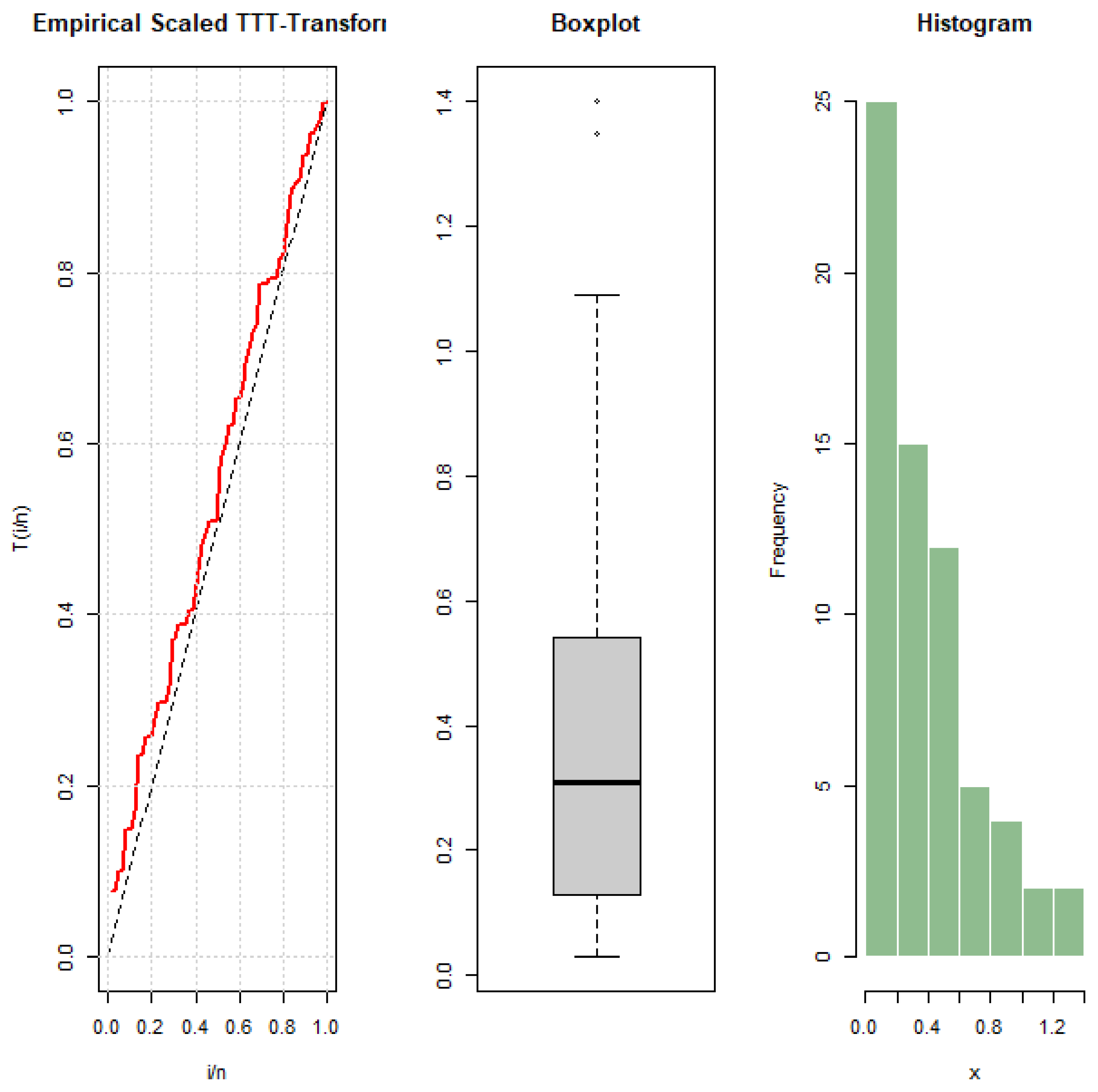
Figure 5 presents the empirical scaled TTT-transform, boxplot, and histogram for the first dataset. The TTT plot clearly indicates an increasing hazard-rate function. Furthermore, the boxplot and histogram reveal that the data are positively skewed. These empirical features suggest that the YLE distribution provides a suitable model for the first dataset.

Table 5. The MLEs of the first dataset.

Model	MLEs	−log L
LE	$\widehat{\lambda }=3.2328,\widehat{\beta }=2.2471$	11.5221
YE	$\widehat{\alpha }=1.7388,\widehat{\lambda }=1.5753$	5.9314
YW	$\widehat{\alpha }=1.2682,\widehat{\beta }=2.3521,\widehat{\lambda }=1.1287$	3.8997
K	$\widehat{\alpha }=1.5511,\widehat{\theta }=1.3673,\widehat{\beta }=0.3565$	5.0892
ENH	$\widehat{\alpha }=1.7476,\widehat{\theta }=1.0647,\widehat{\lambda }=1.3026$	3.7640
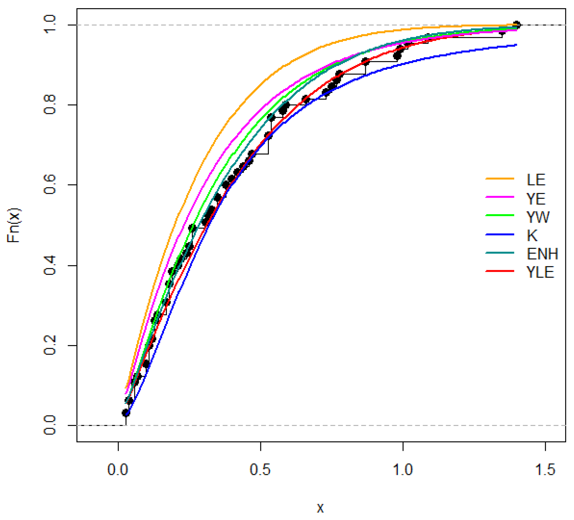
YLE	$\widehat{\alpha }=1.3680,\widehat{\lambda }=1.3486,\widehat{\beta }=1.2101$	3.4878

presents the MLEs and negative log-likelihood values, while

Table 6. The goodness-of-fit statistics for the first dataset.

Model	AIC	CAIC	BIC	HQIC	K-S	p Value
LE	27.0442	27.2377	31.3930	28.7601	0.1916	0.0169
YE	15.8629	16.0564	20.2116	17.5787	0.1292	0.2280
YW	13.7995	14.1929	20.3226	16.3733	0.1082	0.4323
K	16.1785	16.5719	22.7016	18.7523	0.0966	0.5793
ENH	13.5281	13.9215	20.0513	16.1019	0.0880	0.6952
YLE	12.9756	13.3690	19.4987	15.5494	0.0624	0.9619

demonstrates that the YLE distribution provides the lowest AIC, CAIC, BIC, HQIC, and K-S values, and the largest p-value. Therefore, YLE distribution is chosen as the best fit for the first dataset. Figure 6 represents the fitted CDF plots of the YLE, LE, YE, YW, K, and ENH distributions with the empirical distribution for the first dataset.

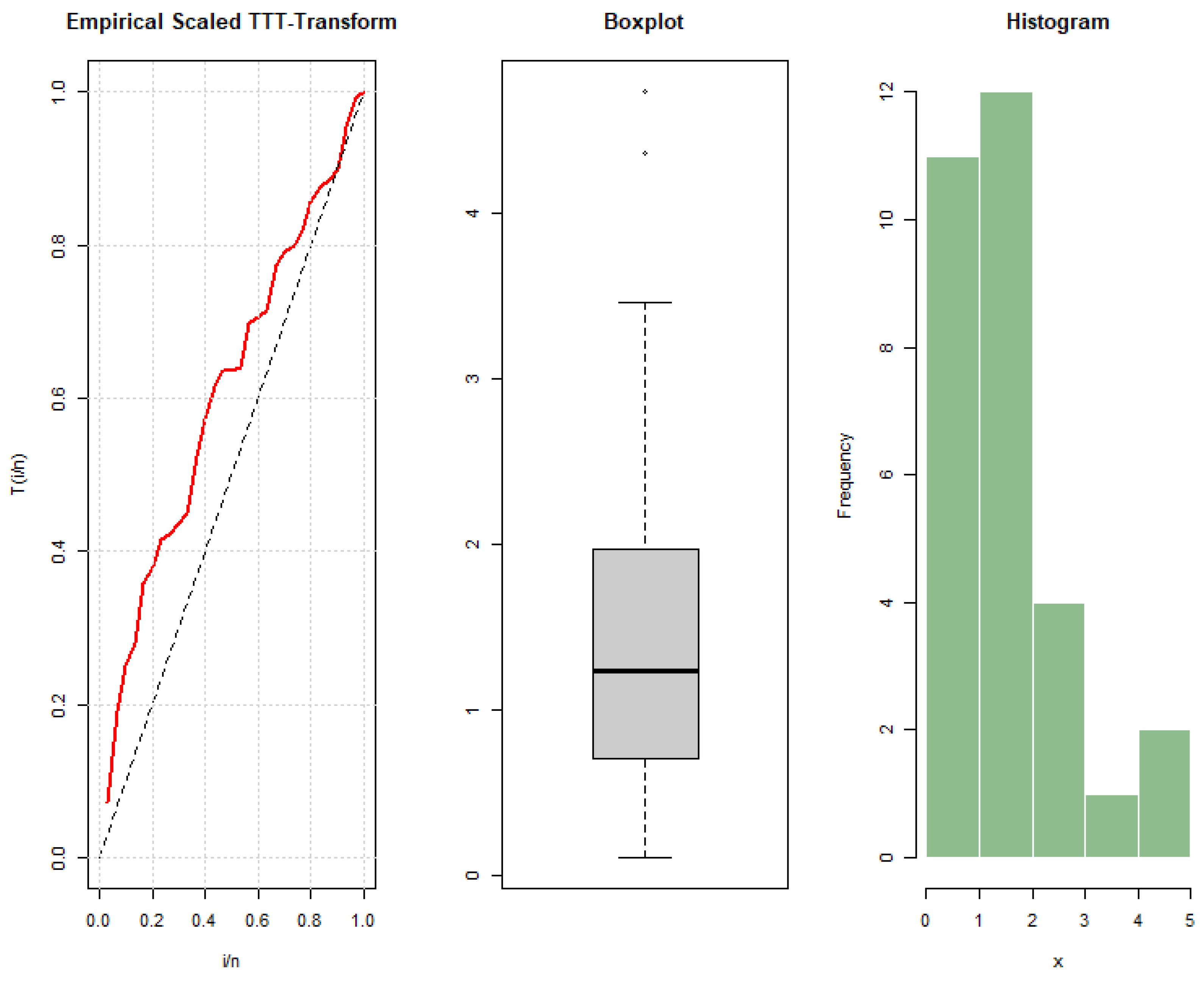
Figure 7 illustrates the empirical scaled TTT-transform, boxplot, and histogram of the second dataset. The TTT plot indicates an increasing hazard-rate function, while the boxplot and histogram reveal a positively skewed distribution with a long right tail. These observations suggest that the YLE distribution is appropriate for modeling the second dataset.

Table 7. The MLEs of the second dataset.

Model	MLEs	−log L
LE	$\widehat{\lambda }=0.4417,\widehat{\beta }=0.8380$	53.1402
YE	$\widehat{\alpha }=2.2313,\widehat{\lambda }=0.2668$	42.3721
YW	$\widehat{\alpha }=2.3051,\widehat{\beta }=0.1327,\widehat{\lambda }=1.9323$	43.1116
K	$\widehat{\alpha }=2.1673,\widehat{\theta }=1.1821,\widehat{\beta }=1.2431$	41.4087
ENH	$\widehat{\alpha }=0.4794,\widehat{\theta }=9.3599,\widehat{\lambda }=9.9317$	43.3507
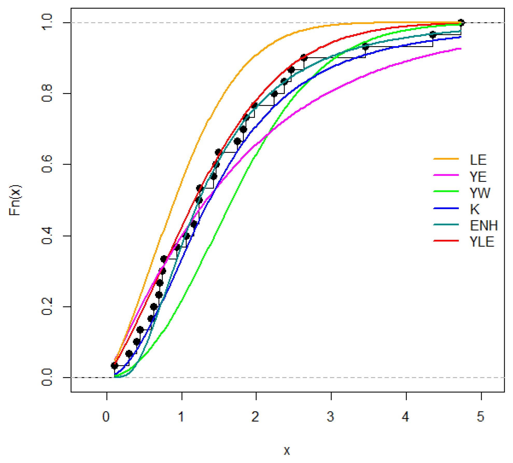
YLE	$\widehat{\alpha }=1.6642,\widehat{\lambda }=0.1630,\widehat{\beta }=0.1801$	40.6386

shows the results of the MLEs and negative log-likelihood values. From

Table 8. The goodness-of-fit statistics for the second dataset.

Model	AIC	CAIC	BIC	HQIC	K-S	p Value
LE	110.2804	110.7249	113.0828	111.1769	0.2639	0.0306
YE	88.7442	89.1886	91.5466	89.6407	0.1828	0.2687
YW	92.2232	93.1463	96.4268	93.5679	0.1574	0.4473
K	88.8174	89.7405	93.0210	90.1622	0.1587	0.4365
ENH	92.7014	93.6245	96.9050	94.0462	0.1447	0.5563
YLE	87.2772	88.2003	91.4808	88.6220	0.0801	0.9906

we can conclude that the YLE distribution provides the lowest AIC, CAIC, BIC, HQIC, and K-S values, and the largest p-value. Therefore, YLE distribution is chosen as the best fit for the second dataset. Figure 8 represents the fitted CDF plots of the YLE, LE, YE, YW, K, and ENH distributions with the empirical distribution for the second dataset.

Overall, this section has demonstrated the practical utility of the proposed YLE distribution through two real-world reliability datasets involving time-between-failure observations. For both datasets, the empirical TTT transforms indicated increasing failure-rate behavior, which is consistent with the flexible hazard-rate structure of the YLE model. Across all considered goodness-of-fit measures, including AIC, CAIC, BIC, HQIC, K-S statistics, and their corresponding p-values, the YLE distribution provided the best overall fit among the competing models. The fitted distribution functions further confirmed the ability of the proposed model to accurately capture the underlying characteristics of the observed data. These results provide strong empirical support for the flexibility, reliability, and applicability of the YLE distribution in lifetime and reliability data analysis.

9. Conclusions

In this paper, we have developed the three-parameter Yun–linear exponential (YLE) distribution by embedding the linear exponential model within the Yun-G family. The study first established the fundamental statistical building blocks of the model, providing explicit analytical expressions for ordinary moments, the moment generating function, and the quantile function. These derivations facilitate a deeper understanding of the model’s structural properties, such as its skewness and kurtosis. Building on this foundation, we established several mathematical characterizations based on truncated moments, hazard functions, and conditional expectations, ensuring the theoretical uniqueness of the YLE model. These characterizations are essential for researchers to verify the theoretical alignment of the YLE model with the underlying stochastic mechanisms of the phenomena under study. In addition, we illustrated the practical applicability of the hazard-based characterization through a diagnostic plot, providing empirical support for the proposed model. Furthermore, we provided a comprehensive analysis of the distribution’s information measures. By deriving explicit expressions for the Rényi entropy, Tsallis entropy, extropy, and cumulative residual entropy (CRE), we have provided a robust framework for quantifying the uncertainty and information content associated with the YLE distribution. For practical implementation, we employed the maximum-likelihood estimation method to estimate the model parameters. The reliability of these estimators was verified through extensive Monte Carlo simulation studies, which confirmed their consistency and efficiency across varying sample sizes. Finally, the empirical utility of the YLE distribution was demonstrated through the analysis of two distinct reliability datasets: MRI scanner failure times and repairable item intervals. Both cases illustrate the flexibility and strong data-modeling capability of the YLE distribution. In future work, the proposed model can be extended by exploring additional characterization techniques and a broader class of information measures, as well as by applying the model to diverse real-world datasets to further assess its practical effectiveness. The proposed model is expected to be useful in a wide range of applications, including engineering, survival and lifetime analysis, meteorology, hydrology, economics, and related fields.

References

1. Glänzel, W. A characterization theorem based on truncated moments and its application to some distribution families. In Mathematical Statistics and Probability Theory; Springer: Berlin/Heidelberg, Germany, 1987; pp. 75–84. [Google Scholar] [CrossRef] [Scilit]
2. Glänzel, W. Some consequences of a characterization theorem based on truncated moments. Statistics 1990, 21, 613–618. [Google Scholar] [CrossRef] [Scilit]
3. Ahsanullah, M. Characterizations of Univariate Continuous Distributions; Atlantis Press: Paris, France, 2017; Volume 7. [Google Scholar]
4. Glänzel, W.; Hamedani, G.G. Characterizations of univariate continuous distributions. Stud. Sci. Math. Hung. 2001, 37, 83–118. [Google Scholar] [CrossRef] [Scilit]
5. Hamedani, G.G. Characterizations of univariate continuous distributions. II. Stud. Sci. Math. Hung. 2002, 39, 407–424. [Google Scholar] [CrossRef] [Scilit]
6. Hamedani, G.G. Characterizations of univariate continuous distributions, III. Stud. Sci. Math. Hung. 2006, 43, 361–385. [Google Scholar] [CrossRef] [Scilit]
7. Hamedani, G.G.; Safavimanesh, F. Characterizations and Infinite Divisibility of Certain 2016 Univariate Continuous Distributions. Int. Math. Forum 2017, 12, 195–228. [Google Scholar] [CrossRef] [Scilit]
8. Ahsanullah, M.; Shakil, M.; Kibria, B.M.G. Characterizations of Continuous Distributions by Truncated Moment. J. Mod. Appl. Stat. Methods 2016, 15, 17. [Google Scholar] [CrossRef] [Scilit]
9. Ahsanullah, M.; Ghitany, M.E.; Al-Mutairi, D.K. Characterization of Lindley Distribution by Truncated Moments. Commun. Stat. Theory Methods 2017, 46, 6222–6227. [Google Scholar] [CrossRef] [Scilit]
10. Hamedani, G.G.; Ahsanullah, M. Characterizations of univariate continuous distributions based on hazard functions II. J. Stat. Theory Appl. 2005, 4, 218–238. [Google Scholar]
11. Jayakumar, K.; Krishnan, B.; Hamedani, G.G. On a New Generalization of Pareto Distribution and Its Applications. Commun. Stat. Simul. Comput. 2020, 49, 1264–1284. [Google Scholar] [CrossRef] [Scilit]
12. Bakouch, H.S.; Hussain, T.; Tošić, M.; Stojanović, V.S.; Qarmalah, N. Unit Exponential Probability Distribution: Characterization and Applications in Environmental and Engineering Data Modeling. Mathematics 2023, 11, 4207. [Google Scholar] [CrossRef] [Scilit]
13. Akhila, P.; Babu, M.G.; Bakouch, H.S. A Versatile Probabilistic Model Based on Yun-G Family of Distributions and Its Applications in Engineering Sector. J. Kerala Stat. Assoc. 2023, 34, 52–83. [Google Scholar]
14. Pillai, J.K.; Joshy, R.C. On Some Aspects of Exponential Intervened Geometric Distribution. Thail. Stat. 2025, 23, 331–354. [Google Scholar]
15. Shannon, C.E. A mathematical theory of communication. Bell Syst. Tech. J. 1948, 27, 379–423. [Google Scholar] [CrossRef] [Scilit]
16. Rényi, A. On measures of entropy and information. In Proceedings of the Fourth Berkeley Symposium on Mathematical Statistics and Probability, Berkeley, CA, USA, 20 June–30 July 1960; University of California Press: Berkeley, CA, USA, 1961; pp. 547–562. [Google Scholar]
17. Tsallis, C.; Mendes, R.S.; Plastino, A.R. The role of constraints within generalized nonextensive statistics. Physical A 1998, 261, 534–554. [Google Scholar] [CrossRef] [Scilit]
18. Lad, F.; Sanfilippo, G.; Agrò, G. Extropy: Complementary dual of entropy. Stat. Sci. 2015, 30, 40–58. [Google Scholar] [CrossRef] [Scilit]
19. Rao, M.; Chen, Y.; Vemuri, B.C.; Wang, F. Cumulative residual entropy: A new measure of information. IEEE Trans. Inf. Theory 2004, 50, 1220–1228. [Google Scholar] [CrossRef] [Scilit]
20. Chesneau, C.; Babu, M.G.; Bakouch, H.S. The Yun transform in probabilistic and statistical contexts: Weibull baseline case and its applications in reliability theory. J. Comput. Math. Data Sci. 2021, 1, 100002. [Google Scholar] [CrossRef] [Scilit]
21. Yun, B.I. An ad hoc approximation to the Gauss error function and a correction method. Appl. Math. Sci. 2014, 8, 4261–4273. [Google Scholar] [CrossRef] [Scilit]
22. Mielke, P.W., Jr. Another family of distributions for describing and analyzing precipitation data. J. Appl. Meteorol. Climatol. 1973, 12, 275–280. [Google Scholar] [CrossRef] [Scilit]
23. Lemonte, A.J. A new exponential-type distribution with constant, decreasing, increasing, upside-down bathtub and bathtub-shaped failure rate function. Comput. Stat. Data Anal. 2013, 62, 149–170. [Google Scholar] [CrossRef] [Scilit]
24. de Negreiros, A.C.S.V.; Lins, I.D.; das Chagas Moura, M.J.; Droguett, E.L. Reliability data analysis of systems in the wear-out phase using a (corrected) q-Exponential likelihood. Reliab. Eng. Syst. Saf. 2020, 197, 106787. [Google Scholar] [CrossRef] [Scilit]
25. Pereira, D.M. Determining the Optimal Replacement of Complex Medical Equipment by Means of Obsolescence Analysis. Master’s Thesis, Universidade Federal de Pernambuco, Recife, Brazil, 2017. (In Portuguese) [Google Scholar]
26. Murthy, D.N.P.; Xie, M.; Jiang, R. Weibull Models; John Wiley & Sons: Hoboken, NJ, USA, 2004. [Google Scholar]
Figure 1. Conceptual framework of the YLE distribution.
Axioms 15 00486 g001
Figure 2. Shapes of the PDF of the YLE distribution for various parameter values: (a) varying λ and β with fixed α ; (b) varying α and λ with fixed β ; (c) varying α and β with fixed λ ; and (d) simultaneous variation of α , λ , and β .
Axioms 15 00486 g002
Figure 3. Shapes of the HRF of the YLE distribution for various parameter values: (a) varying λ and β with fixed α ; (b) varying α and λ with fixed β ; (c) varying α and β with fixed λ ; and (d) simultaneous variation of α , λ , and β .
Axioms 15 00486 g003
Figure 4. The hazard characterization diagnostic plot.
Axioms 15 00486 g004
Figure 5. The empirical scaled TTT-transform, boxplot, and histogram of the first dataset. In the TTT-transform plot, the red solid curve represents the empirical scaled TTT-transform, while the dashed black line denotes the theoretical reference diagonal. In the boxplot, the individual points plotted beyond the whiskers indicate potential outliers.
Axioms 15 00486 g005
Figure 6. Fitted CDF plots for the first dataset. The colored solid curves represent the fitted CDFs of the competing models, while the black dashed line with points represents the empirical CDF of the observed data.
Axioms 15 00486 g006
Figure 7. The empirical scaled TTT-transform, boxplot, and histogram of the second dataset. In the TTT-transform plot, the red solid curve represents the empirical scaled TTT-transform, while the dashed black line denotes the theoretical reference diagonal. In the boxplot, the individual points plotted beyond the whiskers indicate potential outliers.
Axioms 15 00486 g007
Figure 8. Fitted CDF plots for the second dataset. The colored solid curves represent the fitted CDFs of the competing models, while the black dashed line with points represents the empirical CDF of the observed data.
Axioms 15 00486 g008