A Quantitative Hardy Scale for Mixed Local–Fractional Energies and Applications to Singular Schrödinger Forms

Abstract

We develop a quantitative Hardy scale for mixed quadratic energies combining the classical Dirichlet form and a fractional Dirichlet form, ${\mathcal{E}}_{\lambda ,s}\left(u\right)={\int }_{{\mathbb{R}}^n}{|\mathrm{\nabla }u\left(x\right)|}^2\mathrm{d}x+\lambda {\int }_{{\mathbb{R}}^n}{\left|{(-\mathrm{\Delta })}^{s/2}u\left(x\right)\right|}^2\mathrm{d}x,0<s<1,\lambda >0.$ Here, the word scale denotes a parameterized family with a fixed interpolation variable, explicit constants, and the scaling exponent forced by the coexistence of the orders 2 and $2s$. For $n\ge 3$, we prove weighted $L^2$ inequalities indexed by $\gamma \in [s,1]$, which control ${\left|x\right|}^{-2\gamma }$ by ${\mathcal{E}}_{\lambda ,s}$ with the factor ${\lambda }^{-\theta }$, where $\theta =(1-\gamma )/(1-s)$. In dimension $n=2$, the local endpoint is replaced by the logarithmic Hardy weight and gives a mixed log–power family governed by the same parameter. The novelty lies in organizing the endpoint Hardy estimates into a $\lambda$-adapted form suitable for mixed-order operators, with explicit constants, scaling-level optimality of the $\lambda$ exponent, a planar endpoint formulation, and directly usable singular-potential thresholds. The operator consequences are stated at the level of form boundedness, coercivity, spectral lower bounds on bounded domains, semigroup generation, and variational well-posedness; they are presented as consequences of the Hardy scale rather than as a separate spectral theory.

1. Introduction

Hardy inequalities provide quantitative control of singular weights by energy functionals and occupy a central position in elliptic and parabolic equations, spectral theory, and harmonic analysis. In the classical $L^2$ setting on ${\mathbb{R}}^n$ with $n\ge 3$, Hardy’s inequality bounds the inverse-square weight ${\left|x\right|}^{-2}$ by the Dirichlet energy ${\int }_{{\mathbb{R}}^n}{|\mathrm{\nabla }u|}^2$, and the sharp constant is explicitly known [1,2]. This estimate enters the form theory of Schrödinger operators with singular potentials through coercivity and relative form boundedness thresholds [3,4]. Refined versions with remainders, boundary terms, and improved weights remain important in critical elliptic problems [5,6]. Differential equations associated with special polynomial families, including multivariate Hermite polynomials and degenerate Appell-type sequences, provide a complementary operator-theoretic perspective on form domains and spectral theory [7,8].

Fractional analogs replace the gradient energy by the Dirichlet form of a nonlocal operator and control the inverse-power weight ${\left|x\right|}^{-2s}$ through ${\parallel (-\mathrm{\Delta })}^{s/2}{u\parallel }_2^2$. Sharp constants and structural representations are available; one particularly robust route is the ground-state transform, which gives both the constant and a positive nonlocal remainder [9,10]. The Caffarelli–Silvestre extension gives a complementary local realization of the fractional Laplacian [11]. Recent work has expanded fractional Hardy theory toward sharp remainders, $L^p$ frameworks, weighted singular sets, boundary critical cases, and discrete fractional models [12,13]. Recent contributions include weighted fractional Hardy inequalities on flat submanifolds [14], critical fractional boundary Hardy inequalities [15], and optimal discrete fractional Hardy weights [16].

A growing body of work studies operators that superpose local and nonlocal diffusion. A model case is

$$-\mathrm{\Delta }+\lambda {(-\mathrm{\Delta })}^s,0<s<1,\lambda >0,$$

whose quadratic form is

$${\mathcal{E}}_{\lambda ,s}\left(u\right)={\parallel \mathrm{\nabla }u\parallel }_2^2+\lambda {\parallel {(-\mathrm{\Delta })}^{s/2}u\parallel }_2^2.$$

Such mixed symbols occur in Lévy generators with Gaussian and jump parts, jump-diffusion models, anomalous transport, and population models with simultaneous local and long-range dispersal [17,18]. In PDE, mixed local–nonlocal operators have been studied for existence, maximum principles, regularity, shape optimization, Brezis–Oswald- and Brezis–Nirenberg-type problems, and Hardy potential effects [19,20]. The monomiality principle and generating-function methods for polynomial sequences, including Bell-based Apostol–Bernoulli-type polynomials and Gould–Hopper–Frobenius–Genocchi families, offer further tools for analyzing operator recurrences and differential equations arising in such mixed-order settings [21,22]. The more recent literature includes Faber–Krahn and Hong–Krahn–Szegő inequalities for mixed operators [23,24], sublinear and critical mixed problems [25,26], and mixed local–nonlocal equations with Hardy potentials [27,28].

The two terms in ${\mathcal{E}}_{\lambda ,s}$ carry different homogeneities. Under $u_r\left(x\right)=u\left(rx\right)$, the local energy scales like $r^{2-n}$ and the fractional energy scales like $r^{2s-n}$. Thus, $\lambda$ selects a crossover scale between first-order Sobolev control and nonlocal s-order control. Heat-kernel and Green-function estimates for sums of fractional powers provide another view of this multi-regime behavior [29]. For singular weights, this two-scale structure raises a specific quantitative problem: determine which inverse-power weights are controlled by the mixed form, how the control depends on $\lambda$, and how the answer changes at the planar logarithmic endpoint.

The analytical framework developed in this work draws on several foundational and recent contributions across functional analysis, spectral theory, and nonlocal equations. The stability and nonexistence theory for nonlocal elliptic equations involving mixed fractional Laplacians, as examined by Al-Muraqab, Zaidi, and Bouzida [30], provides direct structural parallels to the deformation operators arising in the $\kappa$-setting. The relevance of Lévy-type operators and jump processes to the broader context of non-Gaussian deformations is well illustrated by the financial modelling framework of Cont and Tankov [31], which motivates several of the analytic choices made in the construction of the $\kappa$-Appell family. The treatment of singular integrals and function space embeddings follows the classical framework laid out by Stein [32], while Hardy-type inequalities and the asymptotic behaviour of associated heat semigroups, studied in depth by Vázquez and Zuazua in the inverse-square potential setting [33], inform the spectral estimates used here. The self-adjointness and Fourier-analytic foundations relied upon throughout rest on the methods systematically developed by Reed and Simon [34].

The endpoint inequalities suggest the interval $\gamma \in [s,1]$. The local Hardy inequality controls ${\left|x\right|}^{-2}$, while the fractional Hardy inequality controls ${\left|x\right|}^{-2s}$. A mixed inequality should therefore control ${\left|x\right|}^{-2\gamma }$ for $\gamma$ between these endpoint powers. The direct interpolation argument is simple, but it leaves several useful pieces of information to be organized: the precise $\lambda$ dependence in an additive form, the constants inherited from both endpoints, the interpretation of the interpolation parameter, the scaling limitation on the exponent of $\lambda$, and the planar replacement of ${\left|x\right|}^{-2}$ by a logarithmically corrected weight. This is the gap addressed here. Existing mixed-operator papers typically use mixed Sobolev or Hardy input in problem-specific forms. The present paper isolates a self-contained Hardy scale for the mixed energy and tracks the information needed for form estimates with singular potentials.

The term “Hardy scale” is used in this precise sense: for the single energy ${\mathcal{E}}_{\lambda ,s}$, the paper constructs a one-parameter family of weights joining the local and fractional Hardy endpoints, records multiplicative and additive versions, identifies the scaling exponent $\theta =(1-\gamma )/(1-s)$, and gives the planar log–power analog. The terminology therefore refers to an organized quantitative scale of inequalities, constants, and singular-potential thresholds, rather than to a new class of Hardy spaces.

The contributions are as follows.

• For $n\ge 3$, we prove the mixed Hardy estimate

  $${\int }_{{\mathbb{R}}^n}{\displaystyle \frac{{\left|u\right|}^2}{{\left|x\right|}^{2\gamma }}}\mathrm{d}x\le C_{n,s,\gamma }{\lambda }^{-\theta }{\mathcal{E}}_{\lambda ,s}\left(u\right),\theta ={\displaystyle \frac{1-\gamma }{1-s}},$$

  with an explicit admissible constant in terms of the endpoint Hardy constants.
• We prove that the exponent $\theta$ is forced by the competing homogeneities of $-\mathrm{\Delta }$ and ${(-\mathrm{\Delta })}^s$, giving scaling-level optimality of the $\lambda$ dependence.
• In $n=2$, we replace the local endpoint by the logarithmic Hardy weight and obtain a mixed log–power family with the same parameter $\theta$.
• We give concrete singular-potential examples, coercivity thresholds, spectral lower bounds on bounded domains, semigroup consequences, and shifted variational well-posedness.
• We include numerical and graphical illustrations of the explicit constants and the planar mixed weights.

The paper is organized as follows. Section 2 fixes notation, separates known endpoint inputs from the new mixed estimates, and records the assumptions on n and s. Section 3 establishes the mixed Hardy scale in dimensions $n\ge 3$, including multiplicative and additive estimates and the scaling constraint for the $\lambda$ dependence. Section 4 treats $n=2$ and proves the planar logarithmic mixed family. Section 5 presents consequences for singular Schrödinger forms, including examples, spectral lower bounds, semigroup generation, and shifted variational problems. Section 6 gives quantitative illustrations of the constants and weights. The appendix (Appendix A) records the gamma-function normalization, scaling identities, and the Young inequality used in the proof.

2. Preliminaries: Notation and Standard Tools

Throughout, $n\in \mathbb{N}$, $s\in (0,1)$, and $\lambda >0$. For $u\in L^2\left({\mathbb{R}}^n\right)$, we use the unitary Fourier transform

$$\widehat{u}\left(\xi \right)={\left(2\pi \right)}^{-n/2}{\int }_{{\mathbb{R}}^n}{\mathrm{e}}^{-\mathrm{i}x·\xi }u\left(x\right)\mathrm{d}x,u\left(x\right)={\left(2\pi \right)}^{-n/2}{\int }_{{\mathbb{R}}^n}{\mathrm{e}}^{\mathrm{i}x·\xi }\widehat{u}\left(\xi \right)\mathrm{d}\xi .$$

For $\alpha \ge 0$, define ${(-\mathrm{\Delta })}^{\alpha /2}$ as the Fourier multiplier

$$\widehat{{(-\mathrm{\Delta })}^{\alpha /2}u}\left(\xi \right)={\left|\xi \right|}^{\alpha }\widehat{u}\left(\xi \right),$$

initially on Schwartz functions and extended by density on the natural domains. The notation $\widehat{u}$ is used throughout for this Fourier transform convention. Let

$$H^1\left({\mathbb{R}}^n\right)=\{u\in L^2\left({\mathbb{R}}^n\right):\mathrm{\nabla }u\in L^2\left({\mathbb{R}}^n\right)\},H^s\left({\mathbb{R}}^n\right)=\{u\in L^2\left({\mathbb{R}}^n\right):{(-\mathrm{\Delta })}^{s/2}u\in L^2\left({\mathbb{R}}^n\right)\}.$$

Definition 1

(Mixed energy space). Define

$$X_{\lambda ,s}:=H^1\left({\mathbb{R}}^n\right)\cap H^s\left({\mathbb{R}}^n\right),{\parallel u\parallel }_{X_{\lambda ,s}}^2:={\parallel \mathrm{\nabla }u\parallel }_2^2{+\lambda \parallel (-\mathrm{\Delta })}^{s/2}{u\parallel }_2^2+{\parallel u\parallel }_2^2.$$

Define also the homogeneous mixed energy

$${\mathcal{E}}_{\lambda ,s}\left(u\right):={\parallel \mathrm{\nabla }u\parallel }_2^2+\lambda {\parallel {(-\mathrm{\Delta })}^{s/2}u\parallel }_2^2,u\in X_{\lambda ,s}.$$

The space $X_{\lambda ,s}$ is the form domain of the positive self-adjoint Fourier multiplier with symbol ${\left|\xi \right|}^2+\lambda {\left|\xi \right|}^{2s}$. This makes it the natural energy class for $-\mathrm{\Delta }+\lambda {(-\mathrm{\Delta })}^s$: the first term gives local $H^1$ control, the second term gives fractional $H^s$ control, and the $L^2$ term completes the norm used in resolvent estimates. Since $H^1\left({\mathbb{R}}^n\right)\subset H^s\left({\mathbb{R}}^n\right)$ for $0<s<1$, the underlying set equals $H^1\left({\mathbb{R}}^n\right)$, while the displayed norm keeps the dependence on the mixing parameter $\lambda$ explicit.

Known endpoint results are stated as theorems in this section. The mixed Hardy inequalities, their additive $\lambda$-adapted form, the planar log–power scale, and the operator consequences are the contributions developed in the subsequent sections.

We shall use the following standard endpoint inequalities. The classical estimate is standard [1,2]. The fractional sharp constant follows the fractional Hardy theory [9,10]. The planar logarithmic endpoint follows the logarithmic Hardy framework [3,6].

Theorem 1

(Classical Hardy inequality in ${\mathbb{R}}^n$). Let $n\ge 3$ and $u\in C_c^{\infty }({\mathbb{R}}^n\setminus \left\{0\right\})$. Then

$${\int }_{{\mathbb{R}}^n}{\displaystyle \frac{{\left|u\left(x\right)\right|}^2}{{\left|x\right|}^2}}\mathrm{d}x\le {\displaystyle \frac{4}{{(n-2)}^2}}{\int }_{{\mathbb{R}}^n}{|\mathrm{\nabla }u\left(x\right)|}^2\mathrm{d}x.$$

(1)

Theorem 2

(Fractional Hardy inequality in ${\mathbb{R}}^n$). Assume $s\in (0,1)$ and $2s<n$. For $u\in C_c^{\infty }({\mathbb{R}}^n\setminus \left\{0\right\})$,

$${\int }_{{\mathbb{R}}^n}{\left|{(-\mathrm{\Delta })}^{s/2}u\left(x\right)\right|}^2\mathrm{d}x\ge {\mathcal{H}}_{n,s}{\int }_{{\mathbb{R}}^n}{\displaystyle \frac{{\left|u\left(x\right)\right|}^2}{{\left|x\right|}^{2s}}}\mathrm{d}x,$$

(2)

where the sharp constant is

$${\mathcal{H}}_{n,s}=2^{2s}{\displaystyle \frac{\mathrm{\Gamma }{\left(\frac{n+2s}{4}\right)}^2}{\mathrm{\Gamma }{\left(\frac{n-2s}{4}\right)}^2}}.$$

(3)

Theorem 3

(Planar logarithmic Hardy inequality). In this theorem, the dimension is fixed as $n=2$. Let $B_1=\{x\in {\mathbb{R}}^2:\left|x\right|<1\}$. For $u\in C_c^{\infty }(B_1\setminus \left\{0\right\})$,

$${\int }_{B_1}{\displaystyle \frac{{\left|u\left(x\right)\right|}^2}{{\left|x\right|}^2{\left(log\frac{\mathrm{e}}{\left|x\right|}\right)}^2}}\mathrm{d}x\le 4{\int }_{B_1}{|\mathrm{\nabla }u\left(x\right)|}^2\mathrm{d}x.$$

(4)

For completeness, we record short proofs of the components used later.

Lemma 1

(Proof of Theorem 1). Let $n\ge 3$ and $u\in C_c^{\infty }({\mathbb{R}}^n\setminus \left\{0\right\})$. Then (1) holds.

Proof. 

Let $X\left(x\right)=x/{\left|x\right|}^2$ for $x\ne 0$. A direct computation yields $divX\left(x\right)=(n-2)/{\left|x\right|}^2$. Integration by parts gives

$${\int }_{{\mathbb{R}}^n}{\displaystyle \frac{n-2}{{\left|x\right|}^2}}{\left|u\right|}^2\mathrm{d}x={\int }_{{\mathbb{R}}^n}{(divX)\left|u\right|}^2\mathrm{d}x=-{\int }_{{\mathbb{R}}^n}X·{\mathrm{\nabla }\left(\right|u|}^2)\mathrm{d}x.$$

Since ${\mathrm{\nabla }\left(\right|u|}^2)=2Re(\overline{u}\mathrm{\nabla }u)$, we obtain

$$(n-2){\int }_{{\mathbb{R}}^n}{\displaystyle \frac{{\left|u\right|}^2}{{\left|x\right|}^2}}\mathrm{d}x\le 2{\left({\int }_{{\mathbb{R}}^n}{\displaystyle \frac{{\left|u\right|}^2}{{\left|x\right|}^2}}\mathrm{d}x\right)}^{1/2}{\left({\int }_{{\mathbb{R}}^n}{|\mathrm{\nabla }u|}^2\mathrm{d}x\right)}^{1/2}.$$

If the weighted norm vanishes, there is nothing to prove. Otherwise, divide by its square root and square the result. □

Lemma 2

(Riesz-kernel identity for the ground-state constant). Assume $s\in (0,1)$ and $2s<n$. Define

$${\varphi }_s\left(x\right)={\left|x\right|}^{-(n-2s)/2},x\in {\mathbb{R}}^n\setminus \left\{0\right\}.$$

Then, in the sense of tempered distributions

$${(-\mathrm{\Delta })}^s{\varphi }_s\left(x\right)={\mathcal{H}}_{n,s}{\displaystyle \frac{{\varphi }_s\left(x\right)}{{\left|x\right|}^{2s}}},{\mathcal{H}}_{n,s}=2^{2s}{\displaystyle \frac{\mathrm{\Gamma }{\left(\frac{n+2s}{4}\right)}^2}{\mathrm{\Gamma }{\left(\frac{n-2s}{4}\right)}^2}}.$$

(5)

Proof. 

Set $\alpha =(n+2s)/2$, so that ${\varphi }_s\left(x\right)={\left|x\right|}^{-n+\alpha }$. With the unitary Fourier transform fixed above, the Riesz-kernel identity reads

$$\mathcal{F}\left({\left|x\right|}^{-n+\alpha }\right)\left(\xi \right)=c_{n,\alpha }{\left|\xi \right|}^{-\alpha },0<\alpha <n,$$

where

$$c_{n,\alpha }={\left(2\pi \right)}^{-n/2}{2}^{\alpha }{\pi }^{n/2}{\displaystyle \frac{\mathrm{\Gamma }(\alpha /2)}{\mathrm{\Gamma }\left(\right(n-\alpha )/2)}}.$$

The common factor ${\left(2\pi \right)}^{-n/2}{\pi }^{n/2}$ depends on the Fourier convention and cancels in all ratios below. In distributional language, this identity is obtained by testing against Schwartz functions and then extending the locally integrable kernels by homogeneity.

Multiplication by the symbol ${\left|\xi \right|}^{2s}$ gives

$$\mathcal{F}\left({(-\mathrm{\Delta })}^s{\varphi }_s\right)\left(\xi \right)={\left|\xi \right|}^{2s}\mathcal{F}\left({\varphi }_s\right)\left(\xi \right)=c_{n,\alpha }{\left|\xi \right|}^{2s-\alpha }.$$

Since $2s-\alpha =-(n-2s)/2$, define $\beta =(n-2s)/2$. Then

$$\mathcal{F}\left({(-\mathrm{\Delta })}^s{\varphi }_s\right)\left(\xi \right)=c_{n,\alpha }{\left|\xi \right|}^{-\beta }.$$

Applying the same identity to ${\left|x\right|}^{-n+\beta }$ gives

$$\mathcal{F}\left({\left|x\right|}^{-n+\beta }\right)\left(\xi \right)=c_{n,\beta }{\left|\xi \right|}^{-\beta }.$$

Taking inverse Fourier transforms yields

$${(-\mathrm{\Delta })}^s{\varphi }_s\left(x\right)={\displaystyle \frac{c_{n,\alpha }}{c_{n,\beta }}}{\left|x\right|}^{-n+\beta }.$$

Now ${\left|x\right|}^{-n+\beta }={\left|x\right|}^{-(n+2s)/2}={\varphi }_s\left(x\right){\left|x\right|}^{-2s}$. Moreover

$${\displaystyle \frac{c_{n,\alpha }}{c_{n,\beta }}}=2^{\alpha -\beta }{\displaystyle \frac{\mathrm{\Gamma }(\alpha /2)}{\mathrm{\Gamma }\left(\right(n-\alpha )/2)}}{\displaystyle \frac{\mathrm{\Gamma }\left(\right(n-\beta )/2)}{\mathrm{\Gamma }(\beta /2)}}.$$

Substituting $\alpha =(n+2s)/2$ and $\beta =(n-2s)/2$ gives

$${\displaystyle \frac{c_{n,\alpha }}{c_{n,\beta }}}=2^{2s}{\displaystyle \frac{\mathrm{\Gamma }{\left(\frac{n+2s}{4}\right)}^2}{\mathrm{\Gamma }{\left(\frac{n-2s}{4}\right)}^2}}={\mathcal{H}}_{n,s}.$$

This proves the identity. □

Lemma 3

(Proof of Theorem 2). Assume $s\in (0,1)$ and $2s<n$. For $u\in C_c^{\infty }({\mathbb{R}}^n\setminus \left\{0\right\})$, the inequality (2) holds with the constant (3).

Proof. 

The quadratic form of ${(-\mathrm{\Delta })}^s$ admits the representation

$${\int }_{{\mathbb{R}}^n}{\left|{(-\mathrm{\Delta })}^{s/2}u\left(x\right)\right|}^2\mathrm{d}x={\displaystyle \frac{{\kappa }_{n,s}}{2}}{\int \int }_{{\mathbb{R}}^n\times {\mathbb{R}}^n}{\displaystyle \frac{{|u\left(x\right)-u\left(y\right)|}^2}{{|x-y|}^{n+2s}}}\mathrm{d}x\mathrm{d}y$$

(6)

for the normalization

$${\kappa }_{n,s}={\displaystyle \frac{2^{2s}s\mathrm{\Gamma }\left(\frac{n}{2}+s\right)}{{\pi }^{n/2}\mathrm{\Gamma }(1-s)}}$$

corresponding to the Fourier multiplier ${\left|\xi \right|}^{2s}$ [9,35,36]. Let ${\varphi }_s$ be as in Lemma 2, and set $v=u/{\varphi }_s$.

The following elementary two-point identity is the algebraic core of the ground-state representation: for $a,b\ge 0$ and $z,w\in \mathbb{C}$

$${|az-bw|}^2={ab|z-w|}^2+{(a-b)\left(a\right|z|}^2-{b\left|w\right|}^2).$$

(7)

Applying (7) with $a={\varphi }_s\left(x\right)$, $b={\varphi }_s\left(y\right)$, $z=v\left(x\right)$, and $w=v\left(y\right)$ yields

$$\begin{array}{cc}\hfill {|u\left(x\right)-u\left(y\right)|}^2& ={\varphi }_s\left(x\right){\varphi }_s\left(y\right){|v\left(x\right)-v\left(y\right)|}^2\hfill \\ \hfill & +({\varphi }_s\left(x\right)-{\varphi }_s\left(y\right))\left({\varphi }_s{\left(x\right)\left|v\left(x\right)\right|}^2-{\varphi }_s\left(y\right){\left|v\left(y\right)\right|}^2\right).\hfill \end{array}$$

(8)

Insert (8) into (6). The first term is nonnegative. For the second, symmetrization gives

$${\displaystyle \frac{{\kappa }_{n,s}}{2}}\int \int {\displaystyle \frac{({\varphi }_s\left(x\right)-{\varphi }_s\left(y\right))({\varphi }_s{\left(x\right)\left|v\left(x\right)\right|}^2-{\varphi }_s{\left(y\right)\left|v\left(y\right)\right|}^2)}{{|x-y|}^{n+2s}}}\mathrm{d}x\mathrm{d}y={\int }_{{\mathbb{R}}^n}{\varphi }_s\left(x\right){\left|v\left(x\right)\right|}^2{(-\mathrm{\Delta })}^s{\varphi }_s\left(x\right)\mathrm{d}x.$$

Using Lemma 2

$${(-\mathrm{\Delta })}^s{\varphi }_s\left(x\right)={\mathcal{H}}_{n,s}{\displaystyle \frac{{\varphi }_s\left(x\right)}{{\left|x\right|}^{2s}}},$$

hence

$${\int }_{{\mathbb{R}}^n}{\left|{(-\mathrm{\Delta })}^{s/2}u\right|}^2\mathrm{d}x\ge {\mathcal{H}}_{n,s}{\int }_{{\mathbb{R}}^n}{\displaystyle \frac{{\left|u\left(x\right)\right|}^2}{{\left|x\right|}^{2s}}}\mathrm{d}x.$$

□

Remark 1

(Sharpness of the fractional constant). The constant ${\mathcal{H}}_{n,s}$ is sharp in (2). A standard concentrating sequence is obtained by cutting off the ground-state profile ${\left|x\right|}^{-(n-2s)/2}$ near the origin and at infinity. The ground-state itself is not an admissible $L^2$ test function, which explains why the sharp constant is approached by approximation rather than attained in the homogeneous whole-space inequality.

Lemma 4

(Weighted Hölder factorization). Let $\theta \in [0,1]$ and let $f,g\ge 0$ be measurable. Then

$${\int }_{{\mathbb{R}}^n}f{\left(x\right)}^{1-\theta }g{\left(x\right)}^{\theta }\mathrm{d}x\le {\left({\int }_{{\mathbb{R}}^n}f\left(x\right)\mathrm{d}x\right)}^{1-\theta }{\left({\int }_{{\mathbb{R}}^n}g\left(x\right)\mathrm{d}x\right)}^{\theta }.$$

Proof. 

For $\theta \in (0,1)$, set $p=1/(1-\theta )$ and $q=1/\theta$, so that $1/p+1/q=1$. Then

$${\int }_{{\mathbb{R}}^n}{f}^{1-\theta }{g}^{\theta }={\int }_{{\mathbb{R}}^n}{f}^{1/p}{g}^{1/q}\le {\left({\int }_{{\mathbb{R}}^n}f\right)}^{1/p}{\left({\int }_{{\mathbb{R}}^n}g\right)}^{1/q}.$$

The endpoint cases are immediate. □

3. Main Results in Dimensions $\mathit{n}\ge \mathbf{3}$

We begin by introducing the interpolation parameter

$$\theta =\theta \left(\gamma \right):={\displaystyle \frac{1-\gamma }{1-s}}\in [0,1],\gamma =(1-\theta )·1+\theta ·s,\gamma \in [s,1].$$

(9)

Then

$${\left|x\right|}^{-2\gamma }={\left({\left|x\right|}^{-2}\right)}^{1-\theta }{\left({\left|x\right|}^{-2s}\right)}^{\theta }.$$

Thus, $\theta =0$ selects the local endpoint, $\theta =1$ selects the fractional endpoint, and intermediate values quantify how much of the fractional endpoint is used in the factorization of the weight. Increasing $\gamma$ moves the singularity toward the local inverse-square regime; decreasing $\gamma$ moves it toward the fractional inverse-$2s$ regime. This convention is also the one for which the additive form carries the factor ${\lambda }^{-\theta }$.

Theorem 4

(Mixed Hardy inequality, multiplicative form). Let $n\ge 3$, $s\in (0,1)$, and $\gamma \in [s,1]$, with θ given by (9). For $u\in C_c^{\infty }({\mathbb{R}}^n\setminus \left\{0\right\})$,

$${\int }_{{\mathbb{R}}^n}{\displaystyle \frac{{\left|u\left(x\right)\right|}^2}{{\left|x\right|}^{2\gamma }}}\mathrm{d}x\le {\left({\displaystyle \frac{4}{{(n-2)}^2}}\right)}^{1-\theta }{\left({\displaystyle \frac{1}{{\mathcal{H}}_{n,s}}}\right)}^{\theta }{\parallel \mathrm{\nabla }u\parallel }_2^{2(1-\theta )}{\parallel {(-\mathrm{\Delta })}^{s/2}u\parallel }_2^{2\theta }.$$

(10)

Proof. 

Define

$$f\left(x\right)={\displaystyle \frac{{\left|u\left(x\right)\right|}^2}{{\left|x\right|}^2}},g\left(x\right)={\displaystyle \frac{{\left|u\left(x\right)\right|}^2}{{\left|x\right|}^{2s}}}.$$

Since ${\left|x\right|}^{-2\gamma }={\left|x\right|}^{-2(1-\theta )}{\left|x\right|}^{-2s\theta }$, we have

$${\displaystyle \frac{{\left|u\left(x\right)\right|}^2}{{\left|x\right|}^{2\gamma }}}=f{\left(x\right)}^{1-\theta }g{\left(x\right)}^{\theta }.$$

Applying Lemma 4

$${\int }_{{\mathbb{R}}^n}{\displaystyle \frac{{\left|u\left(x\right)\right|}^2}{{\left|x\right|}^{2\gamma }}}\mathrm{d}x\le {\left({\int }_{{\mathbb{R}}^n}{\displaystyle \frac{{\left|u\left(x\right)\right|}^2}{{\left|x\right|}^2}}\mathrm{d}x\right)}^{1-\theta }{\left({\int }_{{\mathbb{R}}^n}{\displaystyle \frac{{\left|u\left(x\right)\right|}^2}{{\left|x\right|}^{2s}}}\mathrm{d}x\right)}^{\theta }.$$

Now use Theorem 1 and Theorem 2:

$${\int }_{{\mathbb{R}}^n}{\displaystyle \frac{{\left|u\left(x\right)\right|}^2}{{\left|x\right|}^2}}\mathrm{d}x\le {\displaystyle \frac{4}{{(n-2)}^2}}{\parallel \mathrm{\nabla }u\parallel }_2^2,$$

$${\int }_{{\mathbb{R}}^n}{\displaystyle \frac{{\left|u\left(x\right)\right|}^2}{{\left|x\right|}^{2s}}}\mathrm{d}x\le {\displaystyle \frac{1}{{\mathcal{H}}_{n,s}}}{\parallel {(-\mathrm{\Delta })}^{s/2}u\parallel }_2^2.$$

Combining the two estimates gives (10). □

Remark 2

(Meaning of the multiplicative estimate). The proof uses the elementary Hölder factorization of two endpoint Hardy weights. The useful point of Theorem 4 is the way this factorization is tied to the mixed-order energy: the endpoint constants are retained, the parameter θ is fixed by the singular exponent γ, and the estimate is prepared for the λ-dependent additive form in Theorem 5. This organization is the part needed later for singular Schrödinger forms.

Remark 3

(Endpoint recovery). At $\gamma =1$, one has $\theta =0$, and (10) reduces to the classical Hardy inequality. At $\gamma =s$, one has $\theta =1$, and (10) reduces to the fractional Hardy inequality. Thus, the mixed estimate genuinely interpolates between the two endpoint regimes.

Remark 4

(Natural range of the scale). The interval $\gamma \in [s,1]$ is the scale-free interval bounded by the two endpoint Hardy weights controlled by the available energies. For $\gamma >1$, the singularity at the origin is stronger than the inverse-square weight controlled by the first-order part. For $\gamma <s$, a global homogeneous inequality on ${\mathbb{R}}^n$ would require additional far-field control; adding an $L^2$ term leads to a different nonhomogeneous estimate.

Lemma 5

(Weighted Young inequality). Let $A,B\ge 0$, let $\theta \in (0,1)$, and let $\epsilon >0$. Then

$$A^{1-\theta }{B}^{\theta }\le (1-\theta )\epsilon A+\theta {\epsilon }^{-(1-\theta )/\theta }B.$$

(11)

Proof. 

Apply Young’s inequality in the form

$$ab\le {\displaystyle \frac{a^p}{p}}+{\displaystyle \frac{b^q}{q}},{\displaystyle \frac{1}{p}}+{\displaystyle \frac{1}{q}}=1,$$

with $p=1/(1-\theta )$, $q=1/\theta$, $a={\epsilon }^{1/p}{A}^{1/p}$, and $b={\epsilon }^{-1/p}{B}^{1/q}$. □

Theorem 5

(Mixed Hardy inequality, additive form). Let $n\ge 3$, $s\in (0,1)$, and $\gamma \in (s,1)$, with θ given by (9). Then there exists a constant $C_{n,s,\gamma }>0$ such that, for all $u\in C_c^{\infty }({\mathbb{R}}^n\setminus \left\{0\right\})$

$${\int }_{{\mathbb{R}}^n}{\displaystyle \frac{{\left|u\left(x\right)\right|}^2}{{\left|x\right|}^{2\gamma }}}\mathrm{d}x\le C_{n,s,\gamma }{\lambda }^{-\theta }{\mathcal{E}}_{\lambda ,s}\left(u\right),\lambda >0.$$

(12)

A valid explicit choice is

$$C_{n,s,\gamma }={\left({\displaystyle \frac{4}{{(n-2)}^2}}\right)}^{1-\theta }{\left({\displaystyle \frac{1}{{\mathcal{H}}_{n,s}}}\right)}^{\theta }{(1-\theta )}^{1-\theta }{\theta }^{\theta }.$$

(13)

Proof. 

Let

$$K_{n,s,\theta }={\left({\displaystyle \frac{4}{{(n-2)}^2}}\right)}^{1-\theta }{\left({\displaystyle \frac{1}{{\mathcal{H}}_{n,s}}}\right)}^{\theta }.$$

By Theorem 4

$${\int }_{{\mathbb{R}}^n}{\displaystyle \frac{{\left|u\left(x\right)\right|}^2}{{\left|x\right|}^{2\gamma }}}\mathrm{d}x\le K_{n,s,\theta }{\parallel \mathrm{\nabla }u\parallel }_2^{2(1-\theta )}{\parallel {(-\mathrm{\Delta })}^{s/2}u\parallel }_2^{2\theta }.$$

Set

$$A={\parallel \mathrm{\nabla }u\parallel }_2^2,B=\lambda {\parallel {(-\mathrm{\Delta })}^{s/2}u\parallel }_2^2.$$

Then

$${\parallel \mathrm{\nabla }u\parallel }_2^{2(1-\theta )}{\parallel {(-\mathrm{\Delta })}^{s/2}u\parallel }_2^{2\theta }={\lambda }^{-\theta }{A}^{1-\theta }{B}^{\theta }.$$

For fixed $A+B$, the expression $A^{1-\theta }{B}^{\theta }$ is maximized at

$$A=(1-\theta )(A+B),B=\theta (A+B),$$

and therefore

$$A^{1-\theta }{B}^{\theta }\le {(1-\theta )}^{1-\theta }{\theta }^{\theta }(A+B).$$

Thus

$${\int }_{{\mathbb{R}}^n}{\displaystyle \frac{{\left|u\left(x\right)\right|}^2}{{\left|x\right|}^{2\gamma }}}\mathrm{d}x\le C_{n,s,\gamma }{\lambda }^{-\theta }\left({\parallel \mathrm{\nabla }u\parallel }_2^2+\lambda {\parallel {(-\mathrm{\Delta })}^{s/2}u\parallel }_2^2\right),$$

which is (12). □

Remark 5

(Constants in the additive estimate). The constant in (13) optimizes only the elementary passage from the multiplicative product to the sum $A+B$. It inherits the endpoint Hardy constants used in Theorem 4; no sharpness assertion is made for the full intermediate-weight constant. A larger constant is obtained by fixing an arbitrary ε in Lemma 5.

Proposition 1

(Scaling constraint for the $\lambda$-dependence). Assume an inequality of the form

$${\int }_{{\mathbb{R}}^n}{\displaystyle \frac{{\left|u\left(x\right)\right|}^2}{{\left|x\right|}^{2\gamma }}}\mathrm{d}x\le C{\lambda }^{-\alpha }{\mathcal{E}}_{\lambda ,s}\left(u\right)$$

(14)

holds for all $u\in C_c^{\infty }({\mathbb{R}}^n\setminus \left\{0\right\})$, with a constant C independent of $\lambda >0$. Then necessarily

$$\alpha \ge \theta ={\displaystyle \frac{1-\gamma }{1-s}}.$$

In particular, the exponent θ in (12) is optimal at the scaling level.

Proof. 

For $r>0$, let $u_r\left(x\right)=u\left(rx\right)$. Then

$${\int }_{{\mathbb{R}}^n}{\displaystyle \frac{|u_r{\left(x\right)|}^2}{{\left|x\right|}^{2\gamma }}}\mathrm{d}x=r^{2\gamma -n}{\int }_{{\mathbb{R}}^n}{\displaystyle \frac{{\left|u\left(x\right)\right|}^2}{{\left|x\right|}^{2\gamma }}}\mathrm{d}x,$$

$$\parallel \mathrm{\nabla }{u}_r{\parallel }_2^2=r^{2-n}{\parallel \mathrm{\nabla }u\parallel }_2^2{,\parallel (-\mathrm{\Delta })}^{s/2}{u}_r{\parallel }_2^2=r^{2s-n}{\parallel {(-\mathrm{\Delta })}^{s/2}u\parallel }_2^2.$$

Insert $u_r$ into (14):

$$r^{2\gamma -n}{\int }_{{\mathbb{R}}^n}{\displaystyle \frac{{\left|u\right|}^2}{{\left|x\right|}^{2\gamma }}}\mathrm{d}x\le C{\lambda }^{-\alpha }\left(r^{2-n}{\parallel \mathrm{\nabla }u\parallel }_2^2+\lambda r^{2s-n}{\parallel {(-\mathrm{\Delta })}^{s/2}u\parallel }_2^2\right).$$

Choose $r={\lambda }^{1/(2-2s)}$. Then

$$r^{2-n}={\lambda }^{(2-n)/(2-2s)},\lambda r^{2s-n}={\lambda }^{(2-n)/(2-2s)}.$$

Thus, the right-hand side scales like

$${\lambda }^{-\alpha +(2-n)/(2-2s)}.$$

The left-hand side scales like

$${\lambda }^{(2\gamma -n)/(2-2s)}.$$

For the inequality to hold uniformly in $\lambda$, one must have

$${\displaystyle \frac{2\gamma -n}{2-2s}}\ge -\alpha +{\displaystyle \frac{2-n}{2-2s}},$$

which is equivalent to

$$\alpha \ge {\displaystyle \frac{2-2\gamma }{2-2s}}={\displaystyle \frac{1-\gamma }{1-s}}=\theta .$$

□

Remark 6.

The factor ${\lambda }^{-\theta }$ is forced by the mismatch between the local scaling $r^{2-n}$ and the fractional scaling $r^{2s-n}$. Proposition 1 proves scaling optimality of the exponent in estimates with constants independent of λ. Sharpness of the best constant $C_{n,s,\gamma }$ is a separate variational problem and is left open.

4. The Planar Case

In dimension $n=2$, the local endpoint Hardy inequality requires a logarithmic correction. The mixed theory must therefore interpolate between the logarithmically corrected local weight and the pure fractional weight.

Let

$$w_{log}\left(x\right):={\displaystyle \frac{1}{{\left|x\right|}^2{\left(log\frac{\mathrm{e}}{\left|x\right|}\right)}^2}},x\in B_1\setminus \left\{0\right\}.$$

For $\theta \in [0,1]$, define the mixed planar weight

$$W_{\theta ,s}\left(x\right):=w_{log}{\left(x\right)}^{1-\theta }{\left|x\right|}^{-2s\theta }={\displaystyle \frac{1}{{\left|x\right|}^{2(1-\theta +s\theta )}{\left(log\frac{\mathrm{e}}{\left|x\right|}\right)}^{2(1-\theta )}}}.$$

(15)

Since $0<\left|x\right|<1$ on $B_1\setminus \left\{0\right\}$, one has $log(\mathrm{e}/|x\left|\right)>1$; hence, the denominator in (15) is positive throughout the domain of the inequality.

The definition of $W_{\theta ,s}$ is the exact planar analog of the higher-dimensional factorization. The local endpoint weight is $w_{log}$, the fractional endpoint weight is ${\left|x\right|}^{-2s}$, and $W_{\theta ,s}=w_{log}^{1-\theta }{\left|x\right|}^{-2s\theta }$. Hence, the logarithmic correction disappears continuously as $\theta \to 1$, while the full logarithmic Hardy weight is recovered at $\theta =0$.

Theorem 6

(Planar mixed log–power Hardy inequality). Let $s\in (0,1)$ and $\theta \in [0,1]$. For $u\in C_c^{\infty }(B_1\setminus \left\{0\right\})$,

$${\int }_{B_1}{\left|u\left(x\right)\right|}^2{W}_{\theta ,s}\left(x\right)\mathrm{d}x\le 4^{1-\theta }{\mathcal{H}}_{2,s}^{-\theta }{\parallel \mathrm{\nabla }u\parallel }_{L^2\left(B_1\right)}^{2(1-\theta )}{\parallel {(-\mathrm{\Delta })}^{s/2}u\parallel }_{L^2\left({\mathbb{R}}^2\right)}^{2\theta },$$

(16)

where

$${\mathcal{H}}_{2,s}=2^{2s}{\displaystyle \frac{\mathrm{\Gamma }{\left(\frac{1+s}{2}\right)}^2}{\mathrm{\Gamma }{\left(\frac{1-s}{2}\right)}^2}}.$$

Proof. 

By (15)

$${\left|u\left(x\right)\right|}^2{W}_{\theta ,s}\left(x\right)={\left({\displaystyle \frac{{\left|u\left(x\right)\right|}^2}{{\left|x\right|}^2{\left(log\frac{\mathrm{e}}{\left|x\right|}\right)}^2}}\right)}^{1-\theta }{\left({\displaystyle \frac{{\left|u\left(x\right)\right|}^2}{{\left|x\right|}^{2s}}}\right)}^{\theta }.$$

Apply Lemma 4 on $B_1$:

$$\begin{array}{cc}\hfill {\int }_{B_1}{\left|u\left(x\right)\right|}^2{W}_{\theta ,s}\left(x\right)\mathrm{d}x& \le {\left({\int }_{B_1}{\displaystyle \frac{{\left|u\left(x\right)\right|}^2}{{\left|x\right|}^2{\left(log\frac{\mathrm{e}}{\left|x\right|}\right)}^2}}\mathrm{d}x\right)}^{1-\theta }{\left({\int }_{B_1}{\displaystyle \frac{{\left|u\left(x\right)\right|}^2}{{\left|x\right|}^{2s}}}\mathrm{d}x\right)}^{\theta }\hfill \\ \hfill & \le {\left({\int }_{B_1}{\displaystyle \frac{{\left|u\left(x\right)\right|}^2}{{\left|x\right|}^2{\left(log\frac{\mathrm{e}}{\left|x\right|}\right)}^2}}\mathrm{d}x\right)}^{1-\theta }{\left({\int }_{{\mathbb{R}}^2}{\displaystyle \frac{{\left|u\left(x\right)\right|}^2}{{\left|x\right|}^{2s}}}\mathrm{d}x\right)}^{\theta }.\hfill \end{array}$$

Use Theorem 3 and the fractional Hardy inequality in ${\mathbb{R}}^2$:

$${\int }_{B_1}{\displaystyle \frac{{\left|u\left(x\right)\right|}^2}{{\left|x\right|}^2{\left(log\frac{\mathrm{e}}{\left|x\right|}\right)}^2}}\mathrm{d}x\le 4{\parallel \mathrm{\nabla }u\parallel }_{L^2\left(B_1\right)}^2,$$

$${\int }_{{\mathbb{R}}^2}{\displaystyle \frac{{\left|u\left(x\right)\right|}^2}{{\left|x\right|}^{2s}}}\mathrm{d}x\le {\mathcal{H}}_{2,s}^{-1}{\parallel {(-\mathrm{\Delta })}^{s/2}u\parallel }_{L^2\left({\mathbb{R}}^2\right)}^2.$$

Combining the two estimates proves (16). □

Remark 7.

At $\theta =0$, (16) recovers the planar logarithmic Hardy inequality. At $\theta =1$, it reduces to the fractional Hardy inequality in two dimensions. Hence, the planar family interpolates between a logarithmically corrected local endpoint and a pure fractional endpoint.

Remark 8

(On global planar variants). The unit ball is used to fix the logarithmic length scale in the local two-dimensional Hardy endpoint. On a bounded ball $B_R$, the same proof gives the corresponding weight with $log(R\mathrm{e}/|x\left|\right)$. A scale-free global version on all of ${\mathbb{R}}^2$ requires additional confinement, decay, or an external length scale; otherwise, translations and dilations destroy the local logarithmic normalization.

Corollary 1

(Planar additive form). Let $s\in (0,1)$ and $\theta \in (0,1)$. Then there exists $C_{s,\theta }>0$ such that

$${\int }_{B_1}{\left|u\left(x\right)\right|}^2{W}_{\theta ,s}\left(x\right)\mathrm{d}x\le C_{s,\theta }{\lambda }^{-\theta }\left({\parallel \mathrm{\nabla }u\parallel }_{L^2\left(B_1\right)}^2+\lambda {\parallel {(-\mathrm{\Delta })}^{s/2}u\parallel }_{L^2\left({\mathbb{R}}^2\right)}^2\right)$$

(17)

for all $u\in C_c^{\infty }(B_1\setminus \left\{0\right\})$ and all $\lambda >0$.

Proof. 

Combine Theorem 6 with Lemma 5 exactly as in the proof of Theorem 5. □

5. Applications to Singular Schrödinger Forms

We now apply the mixed Hardy inequalities to quadratic forms associated with

$$-\mathrm{\Delta }+\lambda {(-\mathrm{\Delta })}^s-V,$$

where the potential is controlled by an inverse-power singularity. The results in this section are deliberately stated at the form level: they provide explicit thresholds and standard spectral consequences obtained from the mixed Hardy scale.

For $n\ge 3$, let

$$Q_{\lambda ,V}\left[u\right]:={\parallel \mathrm{\nabla }u\parallel }_2^2{+\lambda \parallel (-\mathrm{\Delta })}^{s/2}{u\parallel }_2^2-{\int }_{{\mathbb{R}}^n}V\left(x\right){\left|u\left(x\right)\right|}^2\mathrm{d}x,u\in C_c^{\infty }({\mathbb{R}}^n\setminus \left\{0\right\}).$$

Proposition 2

(Form boundedness for inverse-power potentials). Let $n\ge 3$, let $s\in (0,1)$, and let $\gamma \in [s,1]$. Suppose

$$0\le V\left(x\right)\le {a\left|x\right|}^{-2\gamma }\mathit{a.e.\; on} {\mathbb{R}}^n$$

for some $a>0$. Then

$${\int }_{{\mathbb{R}}^n}V\left(x\right){\left|u\left(x\right)\right|}^2\mathrm{d}x\le a{C}_{n,s,\gamma }{\lambda }^{-\theta }{\mathcal{E}}_{\lambda ,s}\left(u\right)$$

(18)

for every $u\in C_c^{\infty }({\mathbb{R}}^n\setminus \left\{0\right\})$, where $\theta =(1-\gamma )/(1-s)$ and $C_{n,s,\gamma }$ is as in Theorem 5. In particular, V is form bounded with respect to the mixed energy.

Proof. 

Use the pointwise bound $V\left(x\right)\le {a\left|x\right|}^{-2\gamma }$ and then apply Theorem 5. □

Example 1

(Admissible potentials). The hypothesis of Proposition 2 covers the model potential $V\left(x\right)={a\left|x\right|}^{-2\gamma }$ with $\gamma \in [s,1]$. It also covers truncated or softened variants such as

$$V_1\left(x\right)=a{\left|x\right|}^{-2\gamma }{\mathbf{1}}_{B_R}\left(x\right),V_2\left(x\right)={\displaystyle \frac{a}{{\left|x\right|}^{2\gamma }{(1+|log\left|x\right|\left|\right)}^{\delta }}}{\mathbf{1}}_{B_1}\left(x\right),\delta \ge 0,$$

and translated single-center singularities $a|x-x_0{|}^{-2\gamma }$ after applying the same argument with the singular point shifted to $x_0$. If $V=V_s+V_b$ with $0\le V_s\le a{\left|x\right|}^{-2\gamma }$ and $V_b\in L^{\infty }\left({\mathbb{R}}^n\right)$, then

$${\int V|u|}^2\le a{C}_{n,s,\gamma }{\lambda }^{-\theta }{\mathcal{E}}_{\lambda ,s}\left(u\right)+\parallel V_b{\parallel }_{\infty }{\parallel u\parallel }_2^2.$$

Corollary 2

(Coercivity threshold). Under the hypotheses of Proposition 2, if

$${\eta }_{\lambda ,V}:=1-a{C}_{n,s,\gamma }{\lambda }^{-\theta }>0,$$

then

$$Q_{\lambda ,V}\left[u\right]\ge {\eta }_{\lambda ,V}{\mathcal{E}}_{\lambda ,s}\left(u\right)$$

for all $u\in C_c^{\infty }({\mathbb{R}}^n\setminus \left\{0\right\})$. Hence, $Q_{\lambda ,V}$ is coercive on the $X_{\lambda ,s}$ modulo and the $L^2$ part of the norm.

Proof. 

Insert (18) into the definition of $Q_{\lambda ,V}$. □

The threshold can be written as

$$a<C_{n,s,\gamma }^{-1}{\lambda }^{\theta }.$$

For $\gamma =1$, one has $\theta =0$, so the threshold is determined by the local Hardy constant. For $\gamma =s$, one has $\theta =1$, so the admissible size of the singular coefficient grows linearly with $\lambda$. Intermediate powers interpolate between these two regimes.

Theorem 7

(Closed form, spectral lower bound, and semigroup). Let the hypotheses of Proposition 2 hold and assume ${\eta }_{\lambda ,V}>0$. Let $q_{\lambda ,V}$ be the closure of $Q_{\lambda ,V}$ on $X_{\lambda ,s}$ with the form domain $X_{\lambda ,s}$. Then $q_{\lambda ,V}$ is a densely defined, closed, nonnegative symmetric form on $L^2\left({\mathbb{R}}^n\right)$. Consequently, there exists a unique nonnegative self-adjoint operator $H_{\lambda ,V}$ such that

$$q_{\lambda ,V}(u,v)={\langle H_{\lambda ,V}^{1/2}u,H_{\lambda ,V}^{1/2}v\rangle }_{L^2}$$

for $u,v$ in the form domain. Moreover

$$inf\sigma \left(H_{\lambda ,V}\right)\ge 0,{\parallel {\mathrm{e}}^{-t{H}_{\lambda ,V}}\parallel }_{L^2\to L^2}\le 1(t\ge 0),$$

and, for every $\mu >0$

$$\parallel {(H_{\lambda ,V}+\mu )}^{-1}{\parallel }_{L^2\to L^2}\le {\displaystyle \frac{1}{\mu }}.$$

Proof. 

The form associated with $-\mathrm{\Delta }+\lambda {(-\mathrm{\Delta })}^s$ is closed and nonnegative on $X_{\lambda ,s}$. By Proposition 2, the negative potential term has relative bound at most $a{C}_{n,s,\gamma }{\lambda }^{-\theta }<1$ with respect to the mixed energy. The KLMN theorem gives a closed lower-bounded form, and Corollary 2 gives nonnegativity. The first representation theorem gives the self-adjoint operator. The spectral lower bound, contraction of the semigroup, and resolvent estimate follow from the spectral theorem. □

Corollary 3

(Bounded-domain eigenvalue lower bound). Let $\mathrm{\Omega }\subset {\mathbb{R}}^n$ be a bounded Lipschitz domain containing the singular point, and define

$$X_0(\mathrm{\Omega }):=\{u\in X_{\lambda ,s}:u=0\mathit{a.e.\; on}{\mathbb{R}}^n\setminus \mathrm{\Omega }\}.$$

Let $H_{\mathrm{\Omega },\lambda ,V}$ be the self-adjoint operator generated by the restriction of $q_{\lambda ,V}$ to $X_0(\mathrm{\Omega })$. If ${\eta }_{\lambda ,V}>0$, then its first eigenvalue satisfies

$${\lambda }_1\left(H_{\mathrm{\Omega },\lambda ,V}\right)\ge {\eta }_{\lambda ,V}{\mathrm{\Lambda }}_{\mathrm{\Omega },\lambda ,s},$$

where

$${\mathrm{\Lambda }}_{\mathrm{\Omega },\lambda ,s}:=\underset{u\in X_0(\mathrm{\Omega })\setminus \left\{0\right\}}{inf}{\displaystyle \frac{{\mathcal{E}}_{\lambda ,s}\left(u\right)}{{\parallel u\parallel }_2^2}}.$$

In particular

$${\lambda }_1\left(H_{\mathrm{\Omega },\lambda ,V}\right)\ge {\eta }_{\lambda ,V}{\lambda }_1(-\mathrm{\Delta },\mathrm{\Omega }),$$

where ${\lambda }_1(-\mathrm{\Delta },\mathrm{\Omega })$ denotes the first Dirichlet eigenvalue of the local Laplacian.

Proof. 

For $u\in X_0(\mathrm{\Omega })$, Corollary 2 gives $q_{\lambda ,V}\left[u\right]\ge {\eta }_{\lambda ,V}{\mathcal{E}}_{\lambda ,s}\left(u\right)$. Taking the infimum over ${\parallel u\parallel }_2=1$ gives the first bound. Since ${\mathcal{E}}_{\lambda ,s}\left(u\right)\ge {\parallel \mathrm{\nabla }u\parallel }_2^2$, the Rayleigh principle for the Dirichlet Laplacian gives the second bound. □

We next consider a shifted variational problem. Let $\mu >0$ and define

$$B_{\lambda ,V,\mu }(u,v):={\int }_{{\mathbb{R}}^n}\mathrm{\nabla }u·\mathrm{\nabla }\overline{v}\mathrm{d}x+\lambda {\int }_{{\mathbb{R}}^n}{(-\mathrm{\Delta })}^{s/2}u\overline{{(-\mathrm{\Delta })}^{s/2}v}\mathrm{d}x-{\int }_{{\mathbb{R}}^n}Vu\overline{v}\mathrm{d}x+\mu {\int }_{{\mathbb{R}}^n}u\overline{v}\mathrm{d}x.$$

Theorem 8

(Variational well-posedness). Let $n\ge 3$, let $s\in (0,1)$, and let $\gamma \in [s,1]$. Assume

$$0\le V\left(x\right)\le {a\left|x\right|}^{-2\gamma }\mathit{a.e.\; on}{\mathbb{R}}^n$$

with

$$a{C}_{n,s,\gamma }{\lambda }^{-\theta }<1,\theta ={\displaystyle \frac{1-\gamma }{1-s}}.$$

Then for every $F\in X_{\lambda ,s}^{*}$ there exists a unique $u\in X_{\lambda ,s}$ such that

$$B_{\lambda ,V,\mu }(u,v)=F\left(v\right)\mathit{for\; all}v\in X_{\lambda ,s}.$$

(19)

Equivalently, the shifted resolvent problem

$$\left(-\mathrm{\Delta }+\lambda {(-\mathrm{\Delta })}^s-V+\mu \right)u=f$$

is well-posed in the variational sense.

Proof. 

Continuity of $B_{\lambda ,V,\mu }$ on $X_{\lambda ,s}\times X_{\lambda ,s}$ follows from Cauchy–Schwarz and Proposition 2. For coercivity, Corollary 2 gives

$$B_{\lambda ,V,\mu }(u,u)\ge {\eta }_{\lambda ,V}{\mathcal{E}}_{\lambda ,s}\left(u\right)+\mu {\parallel u\parallel }_2^2.$$

Hence

$$B_{\lambda ,V,\mu }(u,u)\ge c{\parallel u\parallel }_{X_{\lambda ,s}}^2$$

for some $c>0$. The Lax–Milgram theorem then yields existence and uniqueness. □

Remark 9

(Uniqueness class). The uniqueness statement is an energy-class statement. Any distributional solution belonging to $X_{\lambda ,s}$ and satisfying the variational identity (19) with the same datum coincides with the Lax–Milgram solution. A lower-regularity uniqueness theory would require a separate transposition or duality framework adapted to the singular potential.

Remark 10.

The same argument applies in the planar setting with the weight $W_{\theta ,s}$ from (15). One obtains corresponding coercivity, spectral, semigroup, and well-posedness statements for singular forms controlled by the mixed log–power Hardy inequality.

6. Quantitative Behavior of the Explicit Constants and Weights

The additive estimate contains the computable constant

$$C_{n,s,\gamma }={\left({\displaystyle \frac{4}{{(n-2)}^2}}\right)}^{1-\theta }{\left({\displaystyle \frac{1}{{\mathcal{H}}_{n,s}}}\right)}^{\theta }{(1-\theta )}^{1-\theta }{\theta }^{\theta },\theta ={\displaystyle \frac{1-\gamma }{1-s}}.$$

The endpoint convention is $0^0=1$ in the factors ${(1-\theta )}^{1-\theta }$ and ${\theta }^{\theta }$. Thus, $C_{n,s,s}={\mathcal{H}}_{n,s}^{-1}$ and $C_{n,s,1}=4/{(n-2)}^2$.

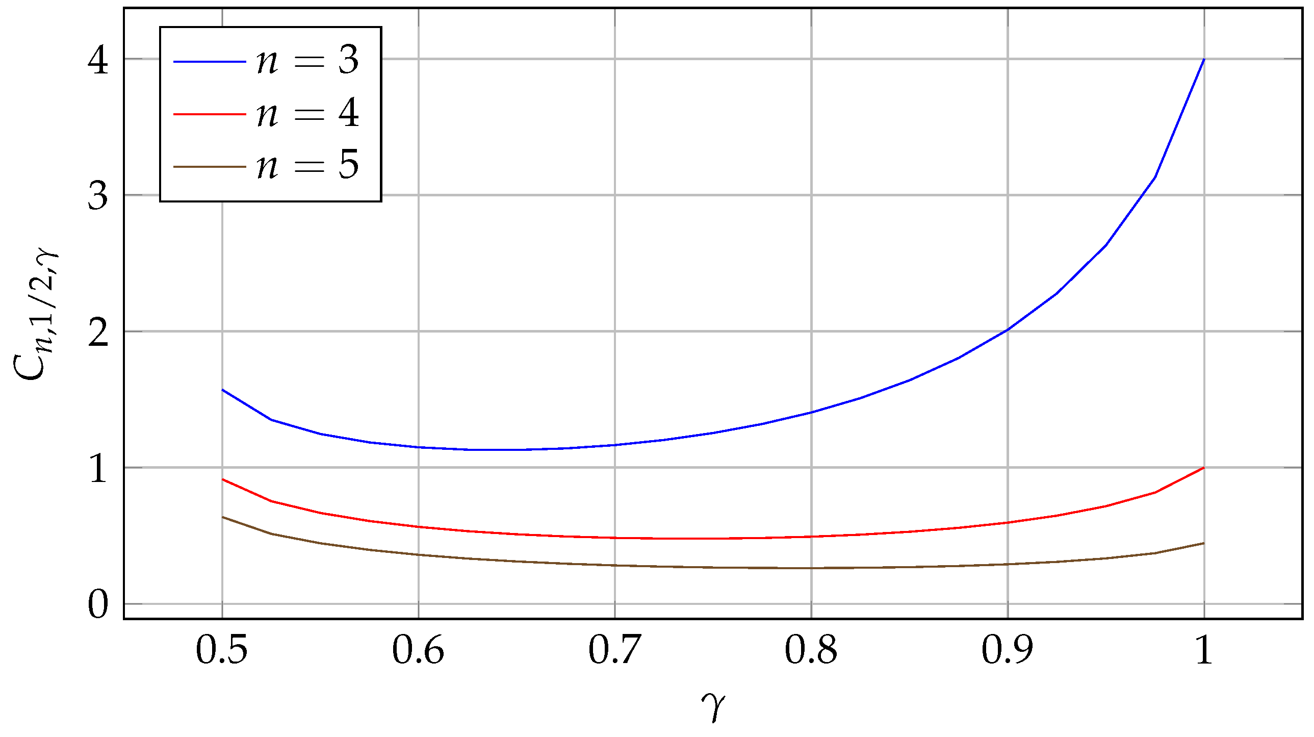
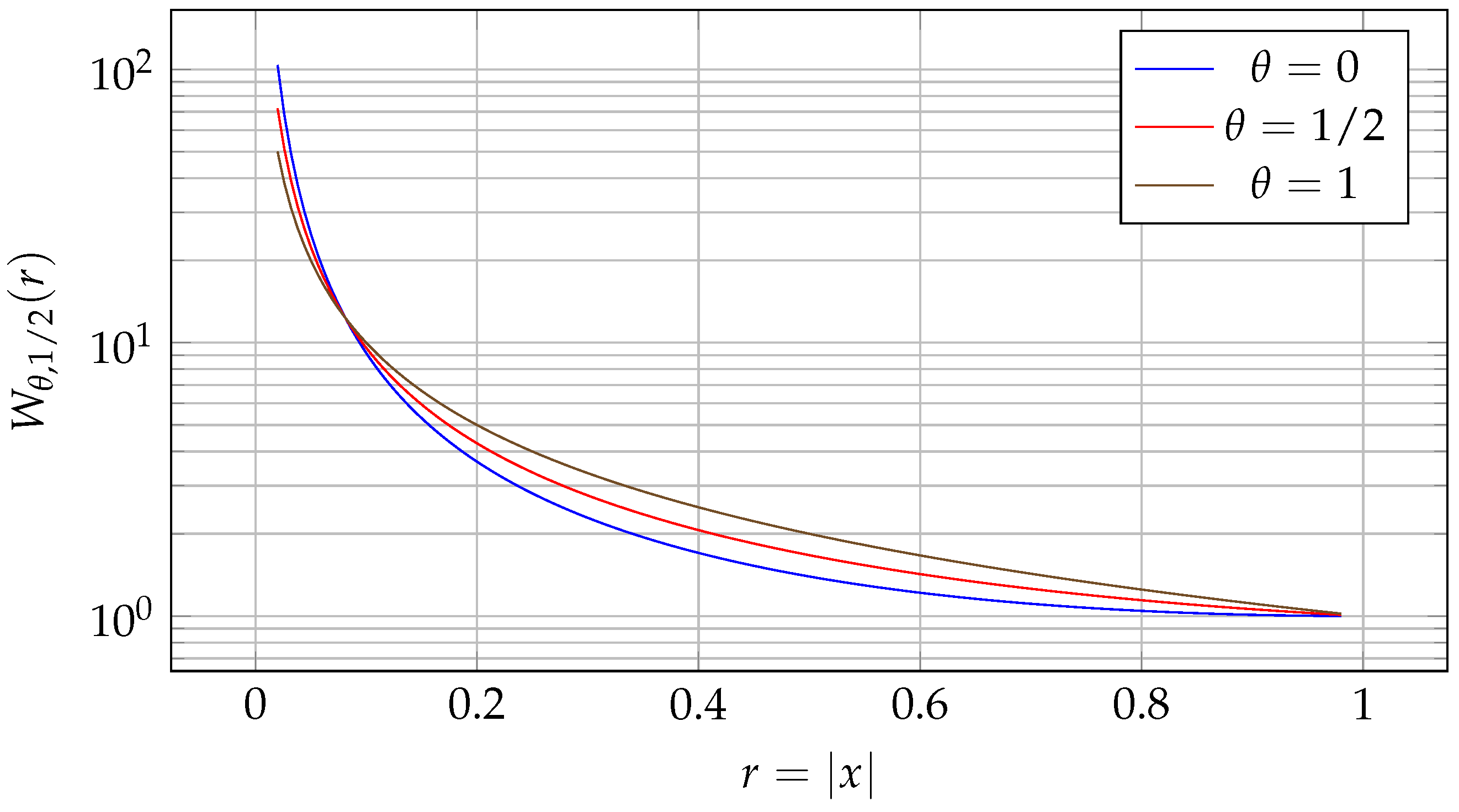
Figure 1 displays the numerical profiles of the explicit additive constant $C_{n,1/2,\gamma }$ for $n=3,4,5$ over $\gamma \in [1/2,1]$, and Figure 2 illustrates the planar mixed weights $W_{\theta ,s}$ for $s=1/2$ and representative values of $\theta$.

For $s=1/2$, the sampled values give

The values illustrate how the local endpoint constant becomes dominant as $\gamma \to 1$, especially in dimension $n=3$ where the classical Hardy constant is 4. Larger dimensions reduce the local endpoint value and shift the minimum toward larger $\gamma$.

The graphical examples have a limited purpose: they display the explicit constants and the shape of the planar weights entering the coercivity threshold. The analytical results remain independent of the sampling grid and of the plotted parameter choices.

7. Conclusions

We established a quantitative Hardy scale for the mixed local–fractional energy

$${\mathcal{E}}_{\lambda ,s}\left(u\right)={\parallel \mathrm{\nabla }u\parallel }_2^2+\lambda {\parallel {(-\mathrm{\Delta })}^{s/2}u\parallel }_2^2.$$

In dimensions $n\ge 3$, this scale controls every intermediate power weight ${\left|x\right|}^{-2\gamma }$ with $\gamma \in [s,1]$. The multiplicative estimate records the endpoint Hardy constants, and the additive estimate isolates the factor ${\lambda }^{-\theta }$ with $\theta =(1-\gamma )/(1-s)$.

The scaling calculation shows why this exponent is the natural one for estimates uniform in $\lambda$. The result is a scaling-optimal statement about the mixing parameter, while the sharp intermediate constants remain a distinct variational question. This distinction keeps the use of optimality limited to what is actually proved.

In dimension $n=2$, the local endpoint is governed by the logarithmic Hardy weight. The mixed planar family interpolates between that logarithmic endpoint and the fractional power weight, producing a log–power scale controlled by the same parameter $\theta$.

The estimates give explicit form bounds for inverse-power singular potentials. They yield coercivity thresholds for Schrödinger forms driven by $-\mathrm{\Delta }+\lambda {(-\mathrm{\Delta })}^s$, self-adjoint nonnegative operators under the subcritical threshold, $L^2$ semigroup bounds, bounded-domain spectral lower bounds, and shifted variational well-posedness. The examples show how the threshold changes with the strength of the fractional component and with the singularity exponent.

Several extensions are natural. Boundary singularities should combine the present mixed scale with boundary Hardy constants. Remainder terms may be approached through the ground-state representation and then inserted into the same multiplicative framework. Spectral questions, including eigenvalue counting and heat-kernel consequences under mixed Hardy potentials, form another concrete direction because the present results already provide the closed-form threshold needed to start such an analysis. More broadly, the degenerate polynomial framework and polynomial differential equations associated with Appell and Frobenius–Genocchi-type families [7,8,21,22] provide operator-theoretic tools that may extend the present Hardy scale to multi-parameter and hybrid settings.

References

1. Hardy, G.H.; Littlewood, J.E.; Pólya, G. Inequalities; Cambridge University Press: Cambridge, UK, 1952. [Google Scholar]
2. Maz’ya, V. Sobolev Spaces with Applications to Elliptic Partial Differential Equations; Springer: Berlin/Heidelberg, Germany, 2011. [Google Scholar]
3. Brezis, H.; Marcus, M. Hardy’s inequalities revisited. Ann. Sc. Norm. Sup. Pisa Cl. Sci. 1997, 25, 217–237. [Google Scholar]
4. Ghoussoub, N.; Moradifam, A. Functional Inequalities: New Perspectives and New Applications; American Mathematical Society: Providence, RI, USA, 2013. [Google Scholar]
5. Filippas, S.; Tertikas, A. Optimizing improved Hardy inequalities. J. Funct. Anal. 2002, 192, 186–233. [Google Scholar] [CrossRef]
6. Del Pino, M.; Dolbeault, J.; Filippas, S.; Tertikas, A. A logarithmic Hardy inequality. J. Funct. Anal. 2010, 259, 2045–2072. [Google Scholar] [CrossRef]
7. Alkahtani, B.S.T.; Alazman, I.; Wani, S.A. Some families of differential equations associated with multivariate Hermite polynomials. Fractal Fract. 2023, 7, 390. [Google Scholar] [CrossRef]
8. Wani, S.A.; Abuasbeh, K.; Oros, G.I.; Trabelsi, S. Degenerate 2D bivariate Appell polynomials: Properties and applications. Appl. Math. Sci. Eng. 2023, 31, 2194645. [Google Scholar] [CrossRef]
9. Frank, R.L.; Seiringer, R. Non-linear ground state representations and sharp Hardy inequalities. J. Funct. Anal. 2008, 255, 3407–3430. [Google Scholar] [CrossRef]
10. Bogdan, K.; Dyda, B. The best constant in a fractional Hardy inequality. Math. Nachr. 2011, 284, 629–638. [Google Scholar] [CrossRef]
11. Caffarelli, L.; Silvestre, L. An extension problem related to the fractional Laplacian. Comm. Partial Differ. Equ. 2007, 32, 1245–1260. [Google Scholar] [CrossRef]
12. Bogdan, K.; Jakubowski, T.; Lenczewska, J.; Pietruska-Pałuba, K. Optimal Hardy inequality for the fractional Laplacian on Lp. J. Funct. Anal. 2022, 282, 109395. [Google Scholar] [CrossRef]
13. Dyda, B.; Kijaczko, M. Sharp fractional Hardy inequalities with a remainder for 1 < p < 2. J. Funct. Anal. 2024, 286, 110373. [Google Scholar] [CrossRef]
14. Sahu, V. Weighted fractional Hardy inequalities with singularity on any flat submanifold. J. Math. Anal. Appl. 2025, 546, 129227. [Google Scholar] [CrossRef]
15. Adimurthi; Roy, P.; Sahu, V. Fractional boundary Hardy inequality for the critical cases. J. Funct. Anal. 2026, 290, 111351. [Google Scholar] [CrossRef]
16. Das, U.; de la Fuente-Fernández, R. An optimal fractional Hardy inequality on the discrete half-line. Calc. Var. Partial Differ. Equ. 2026, 65, 46. [Google Scholar] [CrossRef]
17. Applebaum, D. Lévy Processes and Stochastic Calculus, 2nd ed.; Cambridge University Press: Cambridge, UK, 2009. [Google Scholar]
18. Meerschaert, M.M.; Sikorskii, A. Stochastic Models for Fractional Calculus; De Gruyter: Berlin, Germany, 2012. [Google Scholar]
19. Biagi, S.; Dipierro, S.; Valdinoci, E. Semilinear elliptic equations involving mixed local and nonlocal operators. Proc. Roy. Soc. Edinb. Sect. A 2021, 151, 1611–1641. [Google Scholar]
20. Biagi, S.; Dipierro, S.; Valdinoci, E.; Vecchi, E. Mixed local and nonlocal elliptic operators: Regularity and maximum principles. Comm. Partial Differ. Equ. 2022, 47, 585–629. [Google Scholar]
21. Ramírez, W.; Cesarano, C.; Wani, S.A.; Yousuf, S.; Bedoya, D. About properties and the monomiality principle of Bell-based Apostol–Bernoulli-type polynomials. Carpathian Math. Publ. 2024, 16, 379–390. [Google Scholar]
22. Wani, S.A.; Khan, S.; Nahid, T. Gould–Hopper based Frobenius–Genocchi polynomials and their generalized form. Afr. Mat. 2020, 31, 1397–1408. [Google Scholar]
23. Biagi, S.; Dipierro, S.; Valdinoci, E.; Vecchi, E. A Faber–Krahn inequality for mixed local and nonlocal operators. J. Anal. Math. 2023, 150, 405–448. [Google Scholar]
24. Biagi, S.; Dipierro, S.; Valdinoci, E.; Vecchi, E. A Hong–Krahn–Szegő inequality for mixed local and nonlocal operators. Math. Eng. 2023, 5, 1–25. [Google Scholar]
25. Biagi, S.; Mugnai, D.; Vecchi, E. A Brezis–Oswald approach for mixed local and nonlocal operators. Commun. Contemp. Math. 2024, 26, 2250057. [Google Scholar]
26. Biagi, S.; Dipierro, S.; Valdinoci, E.; Vecchi, E. A Brezis–Nirenberg type result for mixed local and nonlocal operators. NoDEA Nonlinear Differ. Equ. Appl. 2025, 32, 62. [Google Scholar]
27. Biagi, S.; Esposito, F.; Montoro, L.; Vecchi, E. On mixed local–nonlocal problems with Hardy potential. Proc. Roy. Soc. Edinb. Sect. A 2025, 1–34. [Google Scholar] [CrossRef]
28. Malhotra, S.; Goyal, S.; Sreenadh, K. Asymptotic behaviour and existence of positive solutions for mixed local nonlocal elliptic equations with Hardy potential. arXiv 2025, arXiv:2510.04763. [Google Scholar]
29. Chen, Z.-Q.; Kim, P.; Song, R. Dirichlet heat kernel estimates for Δα/2 + Δβ/2. Ill. J. Math. 2010, 54, 1357–1392. [Google Scholar]
30. Al-Muraqab, A.; Zaidi, C.; Bouzida, I. Nonlocal elliptic equations with mixed fractional Laplacians: Stability and nonexistence results. Front. Appl. Math. Stat. 2026, 12, 1826811. [Google Scholar] [CrossRef]
31. Cont, R.; Tankov, P. Financial Modelling with Jump Processes; Chapman and Hall/CRC: Boca Raton, FL, USA, 2004. [Google Scholar]
32. Stein, E.M. Singular Integrals and Differentiability Properties of Functions; Princeton University Press: Princeton, NJ, USA, 1970. [Google Scholar]
33. Vázquez, J.L.; Zuazua, E. The Hardy inequality and the asymptotic behaviour of the heat equation with an inverse-square potential. J. Funct. Anal. 2000, 173, 103–153. [Google Scholar] [CrossRef]
34. Reed, M.; Simon, B. Methods of Modern Mathematical Physics. II: Fourier Analysis, Self-Adjointness; Academic Press: New York, NY, USA, 1975. [Google Scholar]
35. Loss, M.; Sloane, C. Hardy inequalities for fractional integrals on general domains. J. Funct. Anal. 2010, 259, 1369–1379. [Google Scholar] [CrossRef]
36. Lieb, E.H.; Loss, M. Analysis, 2nd ed.; American Mathematical Society: Providence, RI, USA, 2001. [Google Scholar]
Figure 1. Numerical profiles of the explicit additive constant C n , 1 / 2 , γ on γ [ 1 / 2 , 1 ] for n = 3 , 4 , 5 .
Axioms 15 00482 g001
Figure 2. Planar mixed weights W θ , s for s = 1 / 2 and representative values of θ . The logarithmic correction is strongest at the local endpoint θ = 0 and disappears at the fractional endpoint θ = 1 .
Axioms 15 00482 g002
Disclaimer/Publisher’s Note: The statements, opinions and data contained in all publications are solely those of the individual author(s) and contributor(s) and not of MDPI and/or the editor(s). MDPI and/or the editor(s) disclaim responsibility for any injury to people or property resulting from any ideas, methods, instructions or products referred to in the content.