Spline-Based Smoothing of Noisy Discrete Curves in the Frenet–Serret Framework: Sensitivity Analysis of Curvature and Torsion Estimation via CSI and TSI Indices for Analytically Defined Space Curves

Abstract

This study investigates the robustness of Frenet–Serret curvature ($\kappa$) and torsion ($\tau$) estimates derived from noisy discretely-sampled three-dimensional space curves, with emphasis on the comparative performance of cubic spline and cubic Hermite interpolation methods. Accurate estimation of these geometric invariants is essential for reliable analysis of curves arising in signal processing and shape reconstruction; yet, the higher-order derivatives required for their computation exhibit pronounced sensitivity to measurement noise. We examine curves constructed through a Hilbert transform-based parameterization of the form $\mathrm{r}\left(t\right)=\left(X\left(t\right),A\left(t\right)sin\varphi \left(t\right),g\left(t\right)\right),$ where discrete samples are contaminated with additive white Gaussian noise at varying signal-to-noise ratios. Reconstruction is performed using cubic spline interpolation, which ensures global $C^2$ continuity, as well as cubic Hermite spline interpolation, which provides $C^1$ continuity with local tangent control. Frenet frame computations are then applied via regularized finite difference schemes. To characterize noise amplification theoretically, we derive the Curvature Stability Index (CSI) and Torsion Stability Index (TSI) as first-order variance bounds under the delta method. While these indices formalize the derivative-order dependence of noise sensitivity, Monte Carlo simulations reveal that empirical variance exceeds theoretical predictions by factors of ${10}^4$ to ${10}^6$, indicating dominance of nonlinear error propagation. Nevertheless, the indices establish that torsion instability arises fundamentally from third-order derivative structure rather than ground-truth magnitude. Numerical experiments across three geometric regimes constant-invariant helices, variable-curvature helices, and planar curves with identically zero torsion demonstrate that the ratio of the torsion root mean square error to curvature root mean square error consistently ranges from $6.5$ to $9.8$. This disparity persists even in the degenerate planar case, where $\tau \equiv 0$ analytically, confirming that torsion sensitivity is an intrinsic property of the Frenet–Serret formulation. Across all configurations, cubic spline reconstruction yields lower Monte Carlo mean RMSE and reduced empirical variance compared to Hermite spline, providing superior stability for derivative-based invariant estimation.

1. Introduction

The Frenet–Serret frame constitutes a fundamental structure in three-dimensional differential geometry, describing the local behavior of a regular space curve through its unit tangent (T), principal normal (N), and binormal (B) vectors together with the curvature ($\kappa$) and torsion ($\tau$) invariants [1]. These invariants uniquely determine a curve up to rigid motions and play a central role in singularity theory, where variations in curvature and torsion govern the formation of caustics, wavefronts, and envelope-type structures [2,3]. Beyond their geometric interpretation, $\kappa$ and $\tau$ serve as intrinsic descriptors of spatial trajectories and have found applications in physics, geometric modeling, and computational analysis of curves derived from signal processing.

Despite their theoretical clarity, numerical estimation of Frenet–Serret invariants from discrete data remains challenging. Curvature depends on second-order derivatives while torsion involves third-order derivatives, making the latter substantially more sensitive to perturbations. In practical computations, even moderate measurement noise is amplified through successive differentiation, leading to unstable torsion estimates. Such instability has been widely discussed in discrete differential geometry and numerical treatments of singular curve structures [4,5]. Therefore, reliable reconstruction of smooth curves from discrete samples becomes essential before derivative-based invariants can be evaluated in a numerically stable manner.

Spline-based interpolation provides a mathematically rigorous framework for reconstructing smooth curves from discrete observations. Classical cubic spline interpolation guarantees $C^2$ continuity and ensures smooth second derivatives, which is advantageous for curvature computation [6]. In contrast, cubic Hermite splines provide $C^1$ continuity together with explicit control of endpoint tangents, allowing for more localized shape adjustment [7,8]. Since torsion depends on third-order derivatives, the continuity order of the interpolation scheme directly influences numerical stability. Therefore, differences between cubic spline and cubic Hermite spline reconstructions are expected to become more pronounced in torsion estimation compared to curvature evaluation.

The Hilbert transform offers a mechanism for embedding real-valued signals into three-dimensional geometric representations through analytic signal formulation [9]. In such embeddings, the original signal defines one coordinate, while instantaneous amplitude and phase evolution determine the remaining components. This representation transforms temporal signal behavior into spatial trajectories, enabling analysis of signal structures through geometric invariants. However, the robustness of Frenet–Serret invariants under spline-based smoothing of noisy embedded trajectories has not been systematically investigated.

Evaluating robustness under stochastic perturbations is essential for understanding the reliability of derivative-based quantities. The Monte Carlo method, originally introduced by Metropolis and Ulam [10], provides a principled probabilistic framework for studying noise propagation in nonlinear numerical procedures. By generating repeated noisy realizations and recomputing the associated geometric invariants, Monte Carlo simulations enable empirical estimation of variance, stability ranges, and error amplification effects [11]. This approach is particularly relevant for torsion, whose dependence on third-order derivatives makes it theoretically more susceptible to perturbations.

Motivated by these considerations, this study investigates the noise sensitivity of curvature and torsion derived from Frenet–Serret frames applied to noisy discrete curves reconstructed via spline interpolation. Particular emphasis is placed on cubic spline and cubic Hermite spline methods due to their distinct continuity properties and their influence on derivative stability. A central theoretical contribution is the derivation of the Curvature Stability Index (CSI) and the Torsion Stability Index (TSI), which characterize the propagation of perturbations into $\kappa$ and $\tau$ as functions of derivative order.

These indices provide first-order variance bounds under the delta method framework. While they formalize the theoretical relationship between derivative order and noise amplification, the Monte Carlo simulations in Section 3 demonstrate that empirical variance exceeds these bounds by factors of ${10}^4$ to ${10}^6$, indicating that nonlinear noise propagation dominates in practice. Nevertheless, CSI and TSI establish that the stronger instability of torsion arises fundamentally from its third-order derivative structure rather than from large ground-truth magnitudes. This theoretical prediction is subsequently validated through comprehensive Monte Carlo analysis across varying signal-to-noise ratios and multiple geometric configurations.

The remainder of the paper is organized as follows. Section 2 presents the theoretical framework, including the Frenet–Serret formulation and the derivation of CSI and TSI as first-order variance bounds. Section 3 describes the numerical methodology and experimental analysis, encompassing analytical reference validation, spline-based reconstruction under noise, and Monte Carlo stability assessment. Section 4 extends the analysis to variable-curvature and degenerate planar geometries to assess cross-regime generalizability. Section 5 synthesizes the results and discusses the comparative performance of the two spline methods. Section 6 concludes with implications for derivative-based geometric invariant estimation under stochastic perturbations.

2. Frenet–Serret Invariants for the Embedded Curve

Theorem 1. 

Let the curve be defined by

$$\mathrm{r}\left(t\right)=(x\left(t\right),y\left(t\right),z\left(t\right))=\left(t,A\left(t\right)sin\left(\phi \right(t\left)\right),g\left(t\right)\right),$$

(1)

where $A\left(t\right)>0$ is the instantaneous amplitude, $\phi \left(t\right)$ is the phase function, and $g\left(t\right)$ is a smooth scalar function. Define

$$\rho \left(t\right)=\dot{\phi }\left(t\right), v^2\left(t\right)=1+\dot{y}{\left(t\right)}^2+\dot{g}{\left(t\right)}^2,D\left(t\right)=\ddot{y}{\left(t\right)}^2+\ddot{g}{\left(t\right)}^2+{\left(\dot{g}\left(t\right)\ddot{y}\left(t\right)-\ddot{g}\left(t\right)\dot{y}\left(t\right)\right)}^2.$$

(2)

Then, the Frenet–Serret frame {$T\left(t\right),N\left(t\right),B\left(t\right)\}$ and the invariants $\kappa \left(t\right),\tau \left(t\right)$ are given by

$$T\left(t\right)={\displaystyle \frac{1}{\sqrt{v^2\left(t\right)}}}\left(1,\dot{y}\left(t\right),\dot{g}\left(t\right)\right),$$

(3)

$$N\left(t\right)={\displaystyle \frac{1}{\sqrt{v^2\left(t\right)D\left(t\right)}}}\left(-S\left(t\right),-\dot{y}\left(t\right)S\left(t\right)+\ddot{y}\left(t\right)v^2\left(t\right),-\dot{g}\left(t\right)S\left(t\right)+\ddot{g}\left(t\right)v^2\left(t\right)\right),$$

(4)

$$B\left(t\right)={\displaystyle \frac{1}{\sqrt{D\left(t\right)}}}\left(\dot{y}\left(t\right)\ddot{g}\left(t\right)-\dot{g}\left(t\right)\ddot{y}\left(t\right),-\ddot{g}\left(t\right),\ddot{y}\left(t\right)\right),$$

(5)

$$\kappa \left(t\right)={\displaystyle \frac{\sqrt{D\left(t\right)}}{{\left[v^2\left(t\right)\right]}^{3/2}}},$$

(6)

$$\tau \left(t\right)={\displaystyle \frac{-\ddot{g}\left(t\right) y^{\left(3\right)}\left(t\right)+g^{\left(3\right)}\left(t\right)\ddot{y}\left(t\right)}{D\left(t\right)}},$$

(7)

where

$$S\left(t\right)=\dot{g}\left(t\right)\ddot{g}\left(t\right)+\dot{y}\left(t\right)\ddot{y}\left(t\right).$$

Proof of Theorem 1. 

Differentiating $\mathbf{r}\left(t\right)$ gives

$${\mathrm{r}}^{\prime }\left(t\right)=(1,\dot{y}\left(t\right),\dot{g}\left(t\right)), {\parallel {\mathrm{r}}^{\prime }\left(t\right)\parallel }^2=v^2\left(t\right).$$

(8)

Normalization immediately yields the expression for T. The second derivative is

$${\mathrm{r}}^{″}\left(t\right)=(0,\ddot{y}\left(t\right),\ddot{g}\left(t\right)).$$

(9)

Define

$$S\left(t\right)=\dot{g}\left(t\right)\ddot{g}\left(t\right)+\dot{y}\left(t\right)\ddot{y}\left(t\right)={\mathrm{r}}^{\prime }\left(t\right)·{\mathrm{r}}^{″}\left(t\right).$$

The denominator $D\left(t\right)$ is exactly

$$\parallel {\mathrm{r}}^{\prime }\left(t\right)\times {\mathrm{r}}^{″}{\left(t\right)\parallel }^2,$$

which equals the squared area of the parallelogram spanned by the first two derivatives.

The principal normal vector follows from the standard formula

$$N\left(t\right)={\displaystyle \frac{{\mathrm{r}}^{″}\left(t\right)-({\mathrm{r}}^{″}\left(t\right)·\mathrm{T}\left(t\right))\mathrm{T}\left(t\right)}{\parallel {\mathrm{r}}^{″}\left(t\right)-({\mathrm{r}}^{″}\left(t\right)·\mathrm{T}\left(t\right))\mathrm{T}\left(t\right)\parallel }}$$

(10)

after algebraic simplification and substitution of $S\left(t\right)$.

The binormal vector is defined by

$$B\left(t\right)=T\left(t\right)\times N\left(t\right).$$

Direct computation of the cross-product (or the identity $B\propto {\mathrm{r}}^{\prime }\times {\mathrm{r}}^{″}$) yields the simplified form above.

By definition,

$$\kappa \left(t\right)=\parallel T^{\prime }\left(t\right)\parallel ={\displaystyle \frac{\parallel {\mathrm{r}}^{\prime }\left(t\right)\times {\mathrm{r}}^{″}\left(t\right)\parallel }{\parallel {\mathrm{r}}^{\prime }{\left(t\right)\parallel }^3}}={\displaystyle \frac{\sqrt{D\left(t\right)}}{{\left[v^2\left(t\right)\right]}^{3/2}}}.$$

(11)

For torsion, the standard formula reads

$$\tau \left(t\right)={\displaystyle \frac{det({\mathrm{r}}^{\prime }\left(t\right),{\mathrm{r}}^{″}\left(t\right),{\mathrm{r}}^{‴}\left(t\right))}{\parallel {\mathrm{r}}^{\prime }\left(t\right)\times {\mathrm{r}}^{″}{\left(t\right)\parallel }^2}}={\displaystyle \frac{det({\mathrm{r}}^{\prime }\left(t\right),{\mathrm{r}}^{″}\left(t\right),{\mathrm{r}}^{‴}\left(t\right))}{D\left(t\right)}}.$$

(12)

Expanding the determinant along the first row gives

$$det=-\ddot{g}\left(t\right)y^{\left(3\right)}\left(t\right)+g^{\left(3\right)}\left(t\right)\ddot{y}\left(t\right),$$

(13)

which yields the expression for $\tau \left(t\right)$.

Finally, the explicit expressions for the derivatives are

$$\begin{array}{cc}\hfill \dot{y}\left(t\right)& =A^{\prime }\left(t\right)sin\phi \left(t\right)+A\left(t\right)\rho \left(t\right)cos\phi \left(t\right),\hfill \end{array}$$

(14)

$$\begin{array}{cc}\hfill \ddot{y}\left(t\right)& =(A^{″}\left(t\right)-A\left(t\right){\rho }^2\left(t\right))sin\phi \left(t\right)+(2A^{\prime }\left(t\right)\rho \left(t\right)+A\left(t\right){\rho }^{\prime }\left(t\right))cos\phi \left(t\right),\hfill \end{array}$$

(15)

$$\begin{array}{cc}\hfill y^{\left(3\right)}\left(t\right) & =\left(A^{\left(3\right)}\left(t\right)-3A^{\prime }\left(t\right){\rho }^2\left(t\right)-3A\left(t\right)\rho \left(t\right){\rho }^{\prime }\left(t\right)\right)sin\phi \left(t\right)\hfill \\ \hfill & +\left(3A^{″}\left(t\right)\rho \left(t\right)-A\left(t\right){\rho }^3\left(t\right)+3A^{\prime }\left(t\right){\rho }^{\prime }\left(t\right)+A\left(t\right){\rho }^{″}\left(t\right)\right)cos\phi \left(t\right).\hfill \end{array}$$

(16)

This completes the proof. □

2.1. Stability Indices for Curvature and Torsion Under Noise

In the literature, particularly in fiber-optic shape sensing (especially OFDR-based distributed sensing [12,13]), noisy 3D trajectory reconstruction [13] and spline-based interpolation under noise [14,15] have been extensively studied. In these studies, error accumulation and propagation in Frenet–Serret invariants (curvature and torsion) are commonly modeled using partial derivatives, Monte Carlo simulations, or direct assessment of how measurement noise variance affects invariant estimates [14]. Classic references on singularity classification [2,3] discuss how noise can induce spurious fold or cusp-type singularities, while works on discrete curvature/torsion [4,5] and spline fundamentals [6,7,8] provide the background for invariant preservation and smoothing under noise.

The proposed CSI and TSI indices represent a structured derivative-aware extension of these error propagation approaches [16]. They combine local sensitivities derived from Frenet–Serret formulas with the noise variance to provide a practical and interpretable criterion for comparing spline methods (cubic spline, Hermite, Catmull–Rom) in terms of how well they preserve invariant accuracy, especially in regions near degenerate Frenet frames. To quantify the propagation of noise into the Frenet–Serret invariants, we introduce two local indices: the Curvature Sensitivity Index (CSI) and the Torsion Sensitivity Index (TSI). These measures isolate the differential impact of noise in the second and third derivatives of the coordinate function $y\left(t\right)$, respectively.

This extension operates at three distinct levels. First, the derivative-specific decomposition separates the second-order (curvature) and third-order (torsion) contributions, revealing that torsion instability is not merely a consequence of general numerical error but primarily driven by structural amplification through $D{\left(t\right)}^2$ in the denominator. Second, the delta method formulation provides analytical variance approximations that serve as baseline estimates, complementing empirical Monte Carlo simulations that characterize realized dispersion. Third, the pointwise indices $\mathrm{CSI}\left(t\right)$ and $\mathrm{TSI}\left(t\right)$ enable parameter-localized stability assessment near degenerate Frenet frames, while their integral forms $\int \mathrm{CSI}\left(t\right) dt$ and $\int \mathrm{TSI}\left(t\right) dt$ furnish global scalar criteria for method comparison. Together, these components establish a unified framework that captures both local singularity behavior and cumulative reconstruction performance.

Definition 1 (Curvature Stability Index (CSI)). 

Let $\mathbf{r}\left(t\right)$ be the curve defined in (1). The Curvature Stability Index at parameter t is defined as

$$\mathrm{CSI}\left(t\right)={\left|{\displaystyle \frac{\partial \kappa \left(t\right)}{\partial y^{″}\left(t\right)}}\right|}^2{\sigma }^2={\displaystyle \frac{{\left[y^{\prime }\left(t\right)\ddot{g}\left(t\right)-g^{\prime }\left(t\right)y^{″}\left(t\right)\right]}^2}{{\left[v^2\left(t\right)\right]}^3}} {\sigma }^2,$$

(17)

where ${\sigma }^2$ denotes the variance of the additive Gaussian noise and $v^2\left(t\right)=1+\dot{y}{\left(t\right)}^2+\dot{g}{\left(t\right)}^2$.

Theorem 2 (Curvature Stability Index).

The index $\mathit{CSI}\left(t\right)$ follows from the curvature formula $\kappa \left(t\right)=\sqrt{D\left(t\right)}/{\left[v^2\left(t\right)\right]}^{3/2}$.

Proof of Theorem 2. 

By the chain rule,

$${\displaystyle \frac{\partial \kappa \left(t\right)}{\partial y^{″}\left(t\right)}}={\displaystyle \frac{1}{2\sqrt{D\left(t\right)}}}·{\displaystyle \frac{\partial D\left(t\right)}{\partial y^{″}\left(t\right)}}·{\displaystyle \frac{1}{{\left[v^2\left(t\right)\right]}^{3/2}}}.$$

(18)

The partial derivative of $D\left(t\right)$ with respect to $y^{″}\left(t\right)$ is

$${\displaystyle \frac{\partial D\left(t\right)}{\partial y^{″}\left(t\right)}}=2\left[y^{\prime }\left(t\right)\ddot{g}\left(t\right)-g^{\prime }\left(t\right)y^{″}\left(t\right)\right],$$

(19)

yielding

$$\left|{\displaystyle \frac{\partial \kappa \left(t\right)}{\partial y^{″}\left(t\right)}}\right|={\displaystyle \frac{\left|y^{\prime }\left(t\right)\ddot{g}\left(t\right)-g^{\prime }\left(t\right)y^{″}\left(t\right)\right|}{{\left[v^2\left(t\right)\right]}^{3/2}}}.$$

(20)

Applying the delta method [16], the variance of $\kappa \left(t\right)$ induced by a perturbation of variance ${\sigma }^2$ in $y^{″}\left(t\right)$ is approximated as

$$\mathrm{CSI}\left(t\right)=\mathrm{Var}\left(\kappa \left(t\right)\right)\approx {\left|{\displaystyle \frac{\partial \kappa \left(t\right)}{\partial y^{″}\left(t\right)}}\right|}^2{\sigma }^2={\displaystyle \frac{{\left[y^{\prime }\left(t\right)\ddot{g}\left(t\right)-g^{\prime }\left(t\right)y^{″}\left(t\right)\right]}^2}{{\left[v^2\left(t\right)\right]}^3}} {\sigma }^2.$$

(21)

This completes the proof. □

Geometric Interpretation. The quantity $\mathrm{CSI}\left(t\right)$ approximates the variance of $\kappa \left(t\right)$ induced by noise of variance ${\sigma }^2$ in the second-order derivative $y^{″}\left(t\right)$, in the sense of the delta method. When $D\left(t\right)$ is small (near degenerate Frenet frames or fold type singularities), even moderate noise in $y^{″}\left(t\right)$ can substantially increase $\mathrm{CSI}\left(t\right)$, leading to spurious inflection or fold singularities in the extrinsic geometry.

Definition 2 (Torsion Stability Index (TSI)). 

Let $\mathbf{r}\left(t\right)$ be the curve defined in (1). The Torsion Stability Index at parameter t is defined as

$$\mathrm{TSI}\left(t\right)={\left|{\displaystyle \frac{\partial \tau \left(t\right)}{\partial y^{\left(3\right)}\left(t\right)}}\right|}^2{\sigma }^2={\displaystyle \frac{{\left[\ddot{g}\left(t\right)\right]}^2}{{\left[D\left(t\right)\right]}^2}} {\sigma }^2,$$

(22)

where ${\sigma }^2$ denotes the variance of the additive Gaussian noise and $D\left(t\right)$ is defined in (2).

Theorem 3 (Torsion Stability Index).

The index $\mathrm{TSI}\left(t\right)$ follows from the torsion formula in (22).

Proof. 

The torsion is given by

$$\tau \left(t\right)={\displaystyle \frac{-\ddot{g}\left(t\right) y^{\left(3\right)}\left(t\right)+g^{\left(3\right)}\left(t\right) \ddot{y}\left(t\right)}{D\left(t\right)}}.$$

(23)

Taking the partial derivative with respect to $y^{\left(3\right)}\left(t\right)$ yields

$${\displaystyle \frac{\partial \tau \left(t\right)}{\partial y^{\left(3\right)}\left(t\right)}}=-{\displaystyle \frac{\ddot{g}\left(t\right)}{D\left(t\right)}},$$

(24)

since $D\left(t\right)$ and the remaining term $g^{\left(3\right)}\left(t\right) \ddot{y}\left(t\right)$ in the numerator are independent of $y^{\left(3\right)}\left(t\right)$. Therefore,

$$\left|{\displaystyle \frac{\partial \tau \left(t\right)}{\partial y^{\left(3\right)}\left(t\right)}}\right|={\displaystyle \frac{|\ddot{g}\left(t\right)|}{D\left(t\right)}}.$$

(25)

Applying the delta method [16], the variance of $\tau \left(t\right)$ induced by a perturbation of variance ${\sigma }^2$ in $y^{\left(3\right)}\left(t\right)$ is approximated as

$$\mathrm{TSI}\left(t\right)=\mathrm{Var}\left(\tau \left(t\right)\right)\approx {\left|{\displaystyle \frac{\partial \tau \left(t\right)}{\partial y^{\left(3\right)}\left(t\right)}}\right|}^2{\sigma }^2={\displaystyle \frac{{\left[\ddot{g}\left(t\right)\right]}^2}{{\left[D\left(t\right)\right]}^2}} {\sigma }^2.$$

(26)

This completes the proof. □

Geometric Interpretation. The quantity $\mathrm{TSI}\left(t\right)$ approximates the variance of $\tau \left(t\right)$ induced by noise of variance ${\sigma }^2$ in the third-order derivative $y^{\left(3\right)}\left(t\right)$, in the sense of the delta method. In particular, because $D\left(t\right)$ appears squared in the denominator, small values of $D\left(t\right)$ amplify this effect. This ca lead to dramatic sign changes or large fluctuations in $\tau \left(t\right)$, n potentially mimicking spurious cusp or higher-order singularities.

Remarks on Partial Derivatives. The CSI and TSI are defined as variance estimates in the sense of the delta method. Specifically, if $y^{″}\left(t\right)$ is subject to additive noise of variance ${\sigma }^2$, then by the delta method

$$\mathrm{Var}\left(\kappa \left(t\right)\right)\approx {\left|{\displaystyle \frac{\partial \kappa \left(t\right)}{\partial y^{″}\left(t\right)}}\right|}^2{\sigma }^2=\mathrm{CSI}\left(t\right),$$

(27)

and analogously for $\mathrm{TSI}\left(t\right)$ with respect to $y^{\left(3\right)}\left(t\right)$. This formulation is consistent with standard error propagation methodology and directly quantifies the expected variability of the geometric invariants under stochastic perturbations.

Application. The average indices along the curve are defined as the integrals of $\mathrm{CSI}\left(t\right)$ and $\mathrm{TSI}\left(t\right)$ over the parameter interval $[a,b]$:

$${\int }_a^b\mathrm{CSI}\left(t\right) dt, {\int }_a^b\mathrm{TSI}\left(t\right) dt.$$

(28)

Since $\mathrm{CSI}\left(t\right)$ and $\mathrm{TSI}\left(t\right)$ are continuous functions of t, these integrals are approximated numerically using a Riemann sum over a partition $a=t_0<t_1<t_2<\cdots <t_n=b$ with equally spaced points:

$${\int }_a^b\mathrm{CSI}\left(t\right) dt\approx {\displaystyle \frac{b-a}{N}}{\displaystyle \sum _{i=1}^N}\mathrm{CSI}\left(t_i^{*}\right), {\int }_a^b\mathrm{TSI}\left(t\right) dt\approx {\displaystyle \frac{b-a}{N}}{\displaystyle \sum _{i=1}^N}\mathrm{TSI}\left(t_i^{*}\right),$$

(29)

where $t_i^{*}\in [t_{i-1},t_i]$ for $i=1,2,\dots ,N$. These integral-based measures provide quantitative criteria for comparing spline smoothing techniques such as cubic spline, Hermite spline, and Catmull–Rom interpolation in terms of how well they preserve invariant accuracy under noisy conditions.

2.2. Numerical Illustration of Stability Indices (Final Version)

To demonstrate the practical computation of the proposed stability indices, we consider a representative parametric curve constructed from an analytic signal framework. The curve is defined over the interval $t\in [0,2\pi ]$ using $N=200$ equidistant sample points, with the following components:

• Instantaneous amplitude: $A\left(t\right)=1+0.2sin\left(3t\right)$
• Instantaneous phase: $\phi \left(t\right)=t+0.3cos\left(2t\right)$ (mild chirp behavior)
• Third coordinate: $g\left(t\right)=cos\left(t\right)+0.1t^2$ (oscillatory component with quadratic trend).

The resulting parametric curve is given by

$$\mathrm{r}\left(t\right)=(t,A(t)sin\phi (t),g(t\left)\right).$$

To assess the robustness of curvature and torsion under perturbations, additive white Gaussian noise with variance ${\sigma }^2=0.01$ is introduced to the sampled data. Derivatives are evaluated numerically via central finite differences, while the denominator term $D\left(t\right)$ is regularized using a small constant ${10}^{-10}$ to prevent numerical instability.

The computed stability indices over the entire curve yield the following average values:

• Average CSI: $\overline{\mathrm{CSI}}\approx 0.001889$
• Average TSI: $\overline{\mathrm{TSI}}\approx 0.003817$.

Table 1. Selected values of $\mathrm{CSI}\left(t\right)$ and $\mathrm{TSI}\left(t\right)$ at the first five points ($t=0$ to $t\approx 0.126$) for the example curve with ${\sigma }^2=0.01$.

t	CSI (t)	TSI (t)
0.000	0.000690	0.002669
0.032	0.000715	0.002359
0.063	0.000754	0.001987
0.095	0.000808	0.001610
0.126	0.000882	0.001271

presents the values of $\mathrm{CSI}\left(t\right)$ and $\mathrm{TSI}\left(t\right)$ at the first five sample points.

The maximum observed stability values across the curve are:

• Maximum CSI: ≈0.0148
• Maximum TSI: ≈0.1216.

These results clearly indicate that torsion exhibits significantly higher stability compared to curvature under the same noise conditions. While this behavior is theoretically expected due to the involvement of higher-order derivatives, the numerical findings quantitatively demonstrate the extent of this stability within the proposed framework. In particular, the pronounced disparity between CSI and TSI values highlights the practical impact of noise amplification in torsion estimation and underscores the necessity of robust numerical differentiation schemes when dealing with higher-order geometric descriptors.

3. Application

In this section, the Frenet–Serret invariants ($\kappa$, $\tau$) derived in the theoretical framework and the associated stability indices for curvature and torsion (CSI and TSI) are systematically evaluated in a numerical setting. The objective is to examine the behavior of these quantities on an analytically defined reference space curve and to establish a reliable comparison framework for the spline-based reconstruction analysis performed under noisy conditions.

The analysis is carried out in three stages. In the first stage (Step 1), the curvature and torsion of the parametrically defined reference curve are derived in closed form. Subsequently, the CSI and TSI expressions given in Equations (17) and (22) are computed for the selected parameter values. All calculations are implemented in the Python 3.11.7 environment, and the analytical results are validated through graphical representation. This stage provides an exact analytical reference profile for the invariants and their stability measures.

In the second stage (Step 2), discrete samples of the reference curve are generated and Additive White Gaussian Noise (AWGN) is introduced. The noisy data are reconstructed using spline-based techniques, namely, cubic spline and cubic Hermite spline interpolation. Numerical derivatives are computed for each reconstruction, and the corresponding $\kappa$, $\tau$, CSI, and TSI values are obtained. To account for the stochastic nature of noise, Monte Carlo simulations are performed and the statistical distribution of the results is analyzed.

In the third stage (Step 3), the spline-based numerical results are directly compared with the analytical reference values obtained in Step 1. The comparison is conducted both at the local profile level and using global error metrics, including mean absolute error, Root Mean Square (RMS) deviation, and variance. In this way, the theoretical stability analysis is systematically assessed within a numerical and computational framework.

This three-stage methodology ensures that the proposed theoretical framework is examined not only analytically but also computationally and statistically.

3.1. Step 1—Analytical Invariants and Stability Analysis on the Reference Curve

In this step, the analytically defined reference curve

$$\mathrm{r}\left(t\right)=\left(t,-{\displaystyle \frac{1}{{\omega }^2}}sin\left(\omega t\right),-{\displaystyle \frac{1}{{\omega }^2}}cos\left(\omega t\right)\right), t\in [0,4\pi ]$$

(30)

is considered. Throughout this section, $\omega =2$ and ${\sigma }^2=0.01$ are used.

3.1.1. Curvature and Torsion

Using the Frenet–Serret formulas derived in Section 2, the curvature and torsion are obtained in closed form as

$$\kappa ={\displaystyle \frac{{\omega }^2}{{\omega }^2+1}}, \tau =-{\displaystyle \frac{{\omega }^3}{{\omega }^2+1}}.$$

(31)

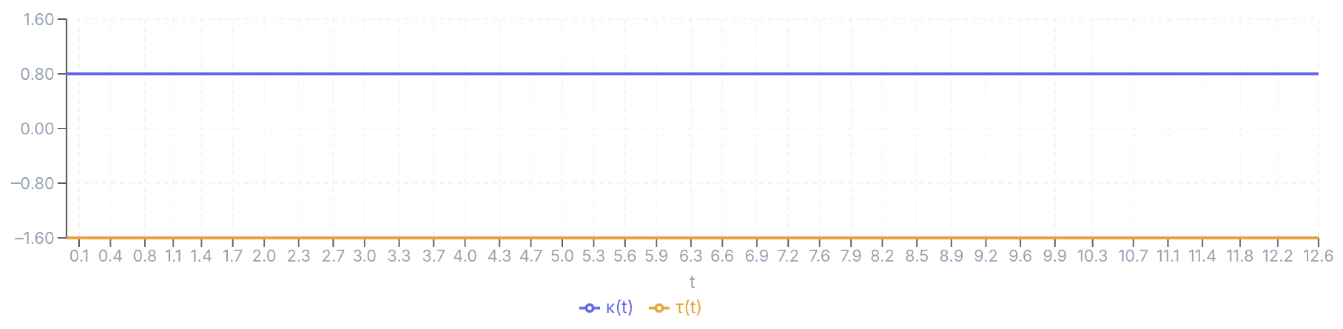
For $\omega =2$, this yields

$$\kappa =0.8, \tau =-1.6.$$

(32)

Both invariants remain constant along the entire parameter interval, confirming the uniform helical structure of the curve. This behavior is illustrated in Figure 1.

3.1.2. Curvature and Torsion Stability Indices

The Curvature Stability Index (CSI) and Torsion Stability Index (TSI), defined in Equations (17) and (22), are computed using the corrected formulations based on squared partial derivatives. For the chosen parameters, the stability indices are obtained as

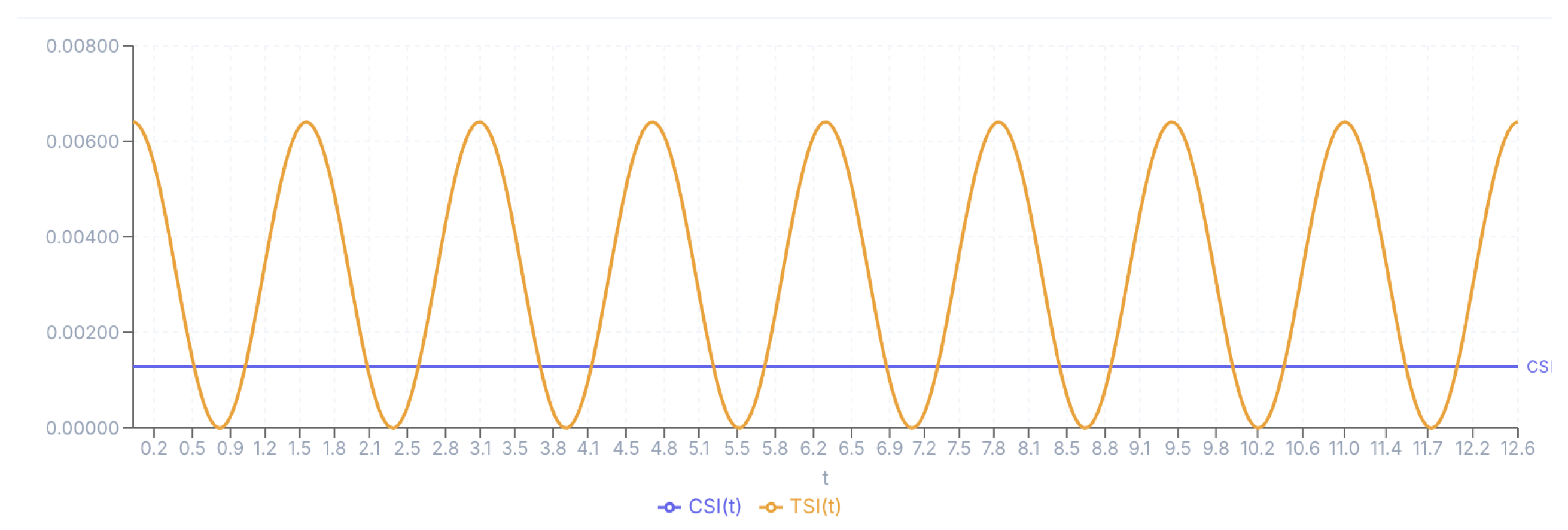
$$\mathrm{CSI}\left(t\right)=0.001280 \left(\mathrm{constant}\right),$$

(33)

$$\mathrm{TSI}\left(t\right)=0.006400{cos}^2\left(2t\right).$$

(34)

Accordingly, CSI remains constant, whereas TSI exhibits periodic oscillations satisfying

$$0\le \mathrm{TSI}\left(t\right)\le 0.006400.$$

(35)

The comparative behavior of the two indices is presented in Figure 2.

3.1.3. Difference Analysis

To quantify the deviation between the two stability measures, the absolute difference

$$\left|\mathrm{CSI}\right(t)-\mathrm{TSI}(t\left)\right|$$

(36)

is evaluated.

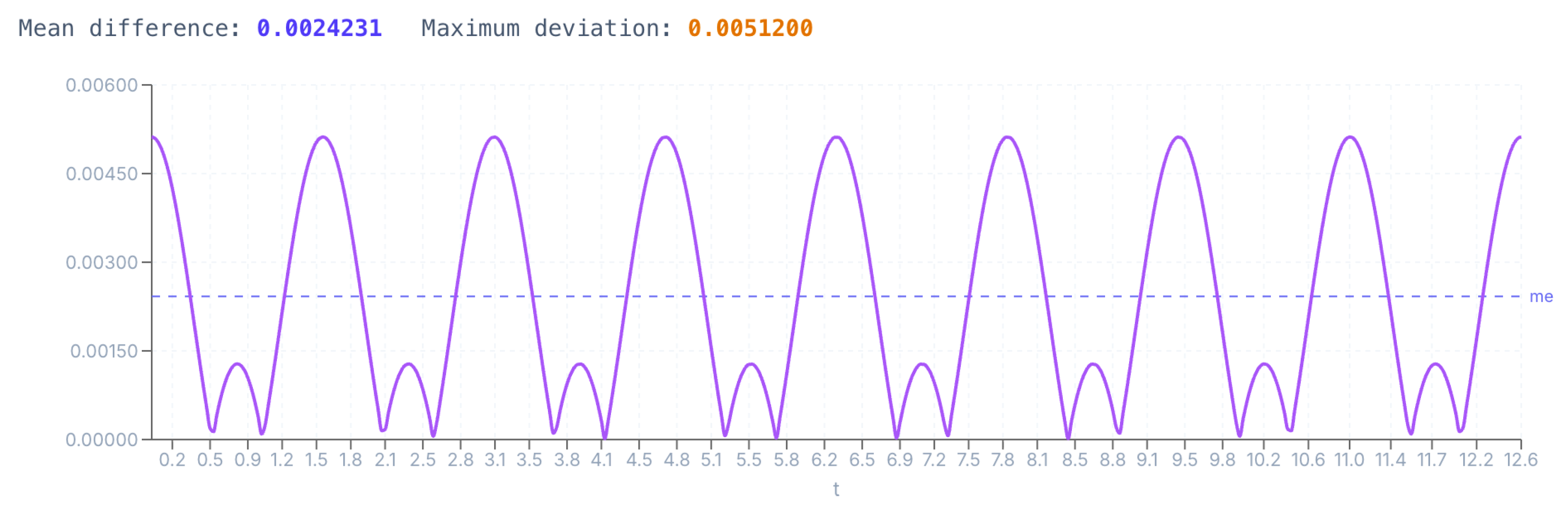
Using the corrected expressions, this difference can be written as

$$|\mathrm{CSI}\left(t\right)-\mathrm{TSI}\left(t\right)|=|0.001280-0.006400{cos}^2\left(2t\right)|.$$

(37)

The mean difference is computed as $0.0024231$, while the maximum deviation is $0.0051200$.

The oscillatory structure of this difference is inherited from the periodic nature of the TSI, and is shown in Figure 3.

3.1.4. Geometric Structure of the Curve

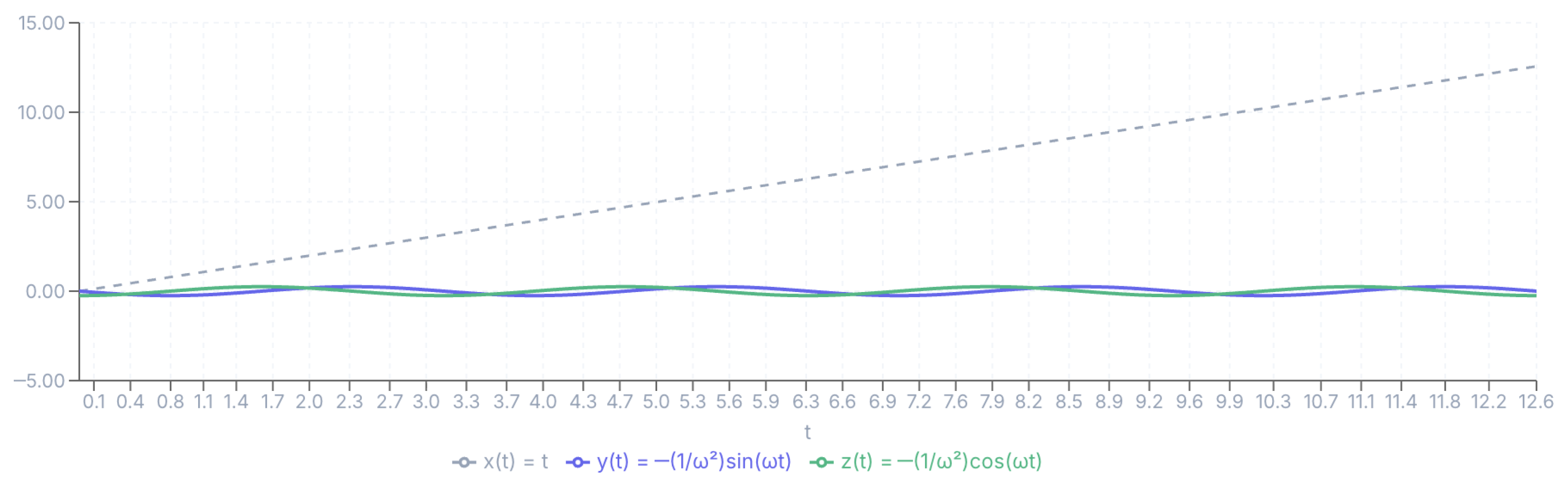
Finally, the transverse components of the reference curve are examined. The functions

$$y\left(t\right)=-{\displaystyle \frac{1}{{\omega }^2}}sin\left(\omega t\right), z\left(t\right)=-{\displaystyle \frac{1}{{\omega }^2}}cos\left(\omega t\right),$$

(38)

exhibit sinusoidal behavior, while the longitudinal component increases linearly.

For $\omega =2$, these reduce to

$$y\left(t\right)=-{\displaystyle \frac{1}{4}}sin\left(2t\right), z\left(t\right)=-{\displaystyle \frac{1}{4}}cos\left(2t\right).$$

(39)

This confirms the helical structure of the curve, as illustrated in Figure 4.

All analytical derivations in this step are exact. The results provide a reliable analytical benchmark for the spline-based reconstruction and Monte Carlo analyses presented in Step 2.

3.2. Step 2—Spline-Based Reconstruction Under Noise

In this stage, discrete samples of the reference curve defined in Step 1 are considered under noise. Cubic spline and Hermite spline approaches are applied to obtain continuous representations of the curve. The objective is to examine how these interpolation schemes influence the associated derivative computations and the behavior of higher-order geometric quantities.

3.2.1. Cubic Spline Reconstruction and Monte Carlo-Based Stability Analysis

Cubic spline interpolation is applied to the analytically defined reference curve, and the statistical stability of curvature ($\kappa$) and torsion ($\tau$) estimates under noise is investigated via Monte Carlo simulations. All numerical computations were implemented in Python using the NumPy and SciPy libraries.

Reference Curve and Frenet–Serret Frame

The reference curve considered in this study is defined as

$$\mathrm{r}\left(t\right)=\left(t,-{\displaystyle \frac{1}{{\omega }^2}}sin\left(\omega t\right),-{\displaystyle \frac{1}{{\omega }^2}}cos\left(\omega t\right)\right), t\in [0,4\pi ].$$

(40)

This parameterization is selected because it is analytically differentiable and permits closed-form computation of all Frenet–Serret quantities, enabling direct comparison between exact geometric invariants and their spline-based numerical approximations. To simulate measurement uncertainty, independent Gaussian noise is added to each sampled point:

$$\tilde{\mathrm{r}}\left(t_i\right)=\mathrm{r}\left(t_i\right)+\sigma {\epsilon }_i, {\epsilon }_i\sim \mathcal{N}(0,{\mathrm{I}}_3)$$

(41)

where $\sigma$ denotes the noise amplitude and ${\mathrm{I}}_3$ represents the $3\times 3$ identity covariance matrix.

The analysis was performed with angular frequency $\omega =2.00$, parameter interval $t\in [0,4\pi ]$ (≈ 12.57), $N=50$ sampling points, noise level $\sigma =0.01$, and $M=40$ Monte Carlo realizations. The choice of $\omega =2$ ensures multiple harmonic oscillations in the y–z plane, allowing for the investigation of derivative-sensitive geometric behavior. The sampling density $N=50$ provides sufficient resolution for spline construction without excessive smoothing, the noise level $\sigma =0.01$ is small relative to the curve amplitude but large enough to expose instability in higher-order derivatives, and $M=40$ provides stable empirical variance estimates across the parameter domain.

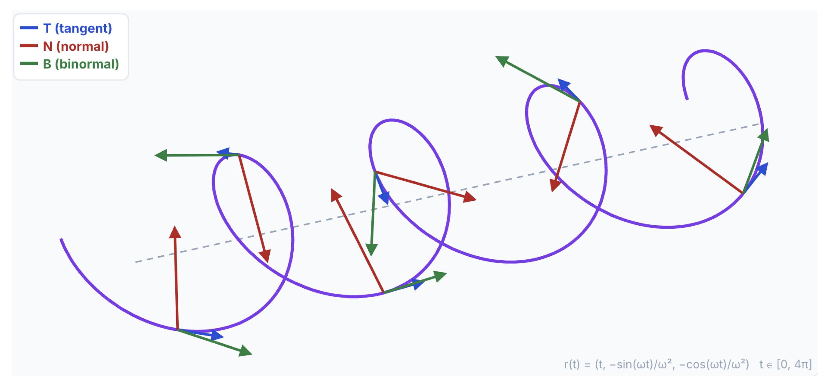
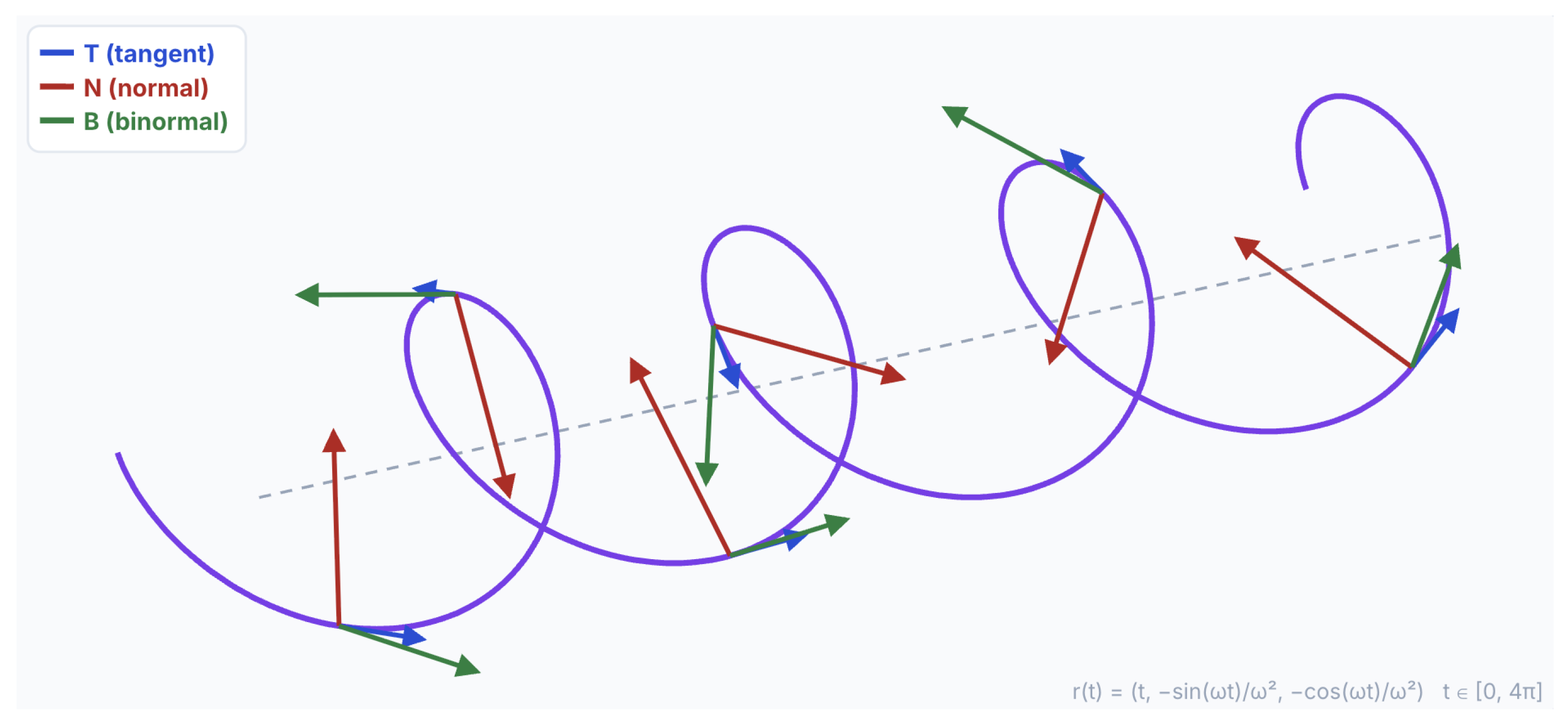
The Frenet–Serret frame associated with the reference curve is visualized in Figure 5 via cavalier oblique projection, with the tangent (T), normal (N), and binormal (B) vectors computed analytically and displayed at uniformly spaced parameter values along the helix.

The frame rotates continuously and smoothly along the curve, reflecting the constant curvature and torsion of the underlying helix. The binormal vector maintains a consistent orientation relative to the helix axis, as expected for a curve with nonzero constant torsion.

Cubic Spline Interpolation

Cubic spline interpolation is constructed separately for each coordinate component of the noisy discrete data. Let ${\left\{t_i\right\}}_{i=1}^N$ denote the sampling points and $\tilde{\mathrm{r}}\left(t_i\right)$ the corresponding noisy observations. For each coordinate function, a natural cubic spline is constructed as a piecewise degree-three polynomial that interpolates the function values at all sampling points, maintains continuity of first and second derivatives across knot points, and satisfies natural boundary conditions by requiring the second derivative to vanish at the endpoints.

The spline representation provides a smooth continuous approximation ${\mathrm{r}}_s\left(t\right)$, from which analytical derivatives ${\mathrm{r}}_s^{\prime }\left(t\right)$, ${\mathrm{r}}_s^{″}\left(t\right)$, and ${\mathrm{r}}_s^{‴}\left(t\right)$ are obtained directly. Curvature and torsion are then computed via the Frenet–Serret formulas:

$$\kappa \left(t\right)={\displaystyle \frac{\parallel {\mathrm{r}}_s^{\prime }\left(t\right)\times {\mathrm{r}}_s^{″}\left(t\right)\parallel }{\parallel {\mathrm{r}}_s^{\prime }{\left(t\right)\parallel }^3}},$$

(42)

$$\tau \left(t\right)={\displaystyle \frac{\left({\mathrm{r}}_s^{\prime }\left(t\right)\times {\mathrm{r}}_s^{″}\left(t\right)\right)·{\mathrm{r}}_s^{‴}\left(t\right)}{\parallel {\mathrm{r}}_s^{\prime }\left(t\right)\times {\mathrm{r}}_s^{″}{\left(t\right)\parallel }^2}}.$$

(43)

Since torsion involves third-order derivatives, it amplifies noise at a rate of $\mathcal{O}(\sigma /h^3)$, compared to $\mathcal{O}(\sigma /h^2)$ for curvature [14,15], implying $\mathrm{Var}\left({\tau }_s\right)>\mathrm{Var}\left({\kappa }_s\right)$ under any noise realization.

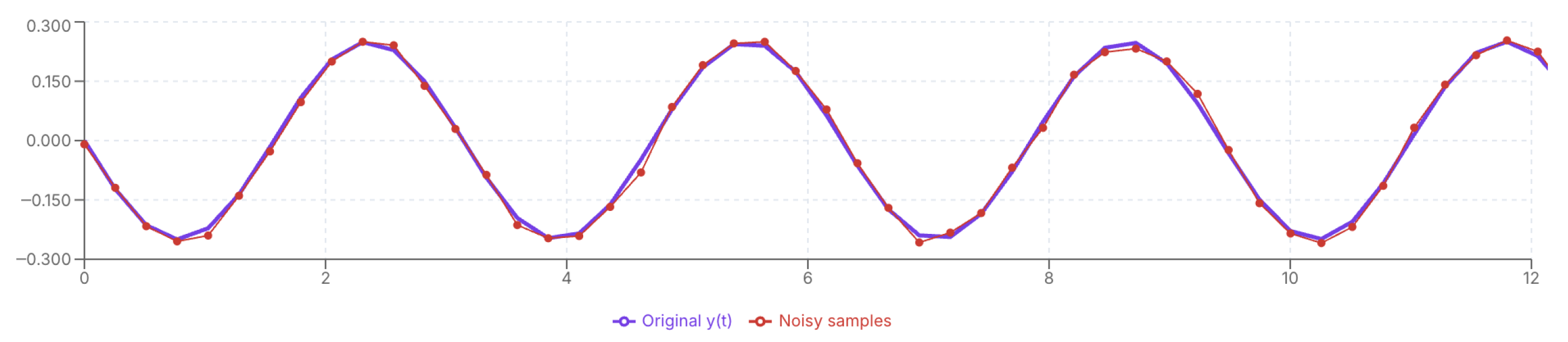
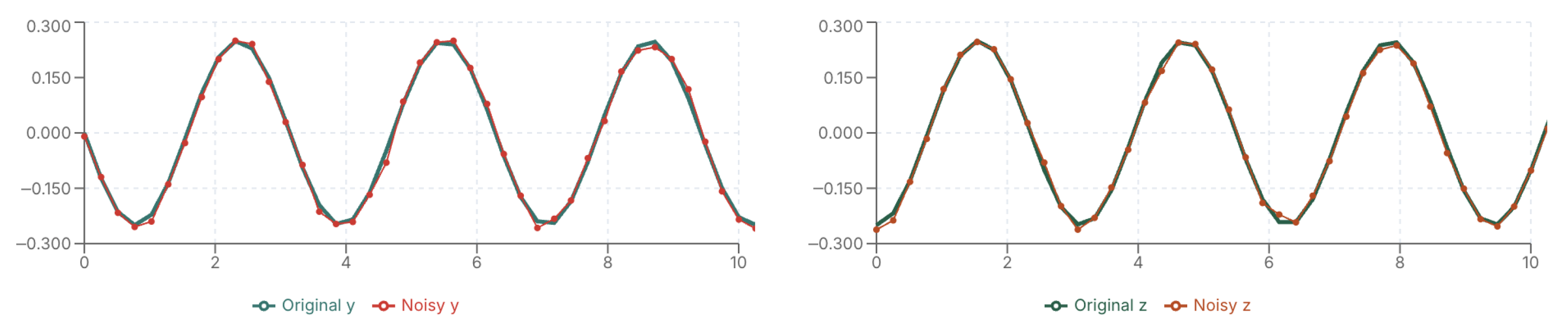
The quality of the spline reconstruction at the function level is examined in Figure 6 and Figure 7. Figure 6 shows the noisy discrete samples alongside the cubic spline fit for the $y\left(t\right)$ component, while Figure 7 presents the component-wise comparison for $y\left(t\right)$ (left panel) and $z\left(t\right)$ (right panel).

The spline reconstruction closely follows the original signal in both components. The linear component $x\left(t\right)=t$ remains unaffected by noise, whereas the sinusoidal components $y\left(t\right)=-{\omega }^{-2}sin\left(\omega t\right)$ and $z\left(t\right)=-{\omega }^{-2}cos\left(\omega t\right)$ exhibit mild deviations near extremum regions, where numerical differentiation is most sensitive to perturbations. Whether this function-level fidelity extends to higher-order derivative quantities is the subject of the subsequent analysis.

Behavior of Curvature and Torsion

The theoretical invariants of the reference helix are constant:

$${\kappa }_{\mathrm{theo}}=0.8000, {\tau }_{\mathrm{theo}}=-1.6000.$$

(44)

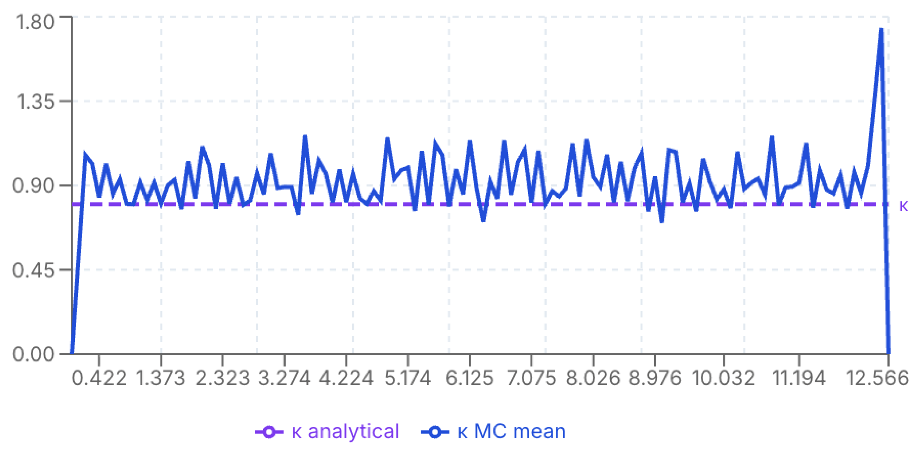
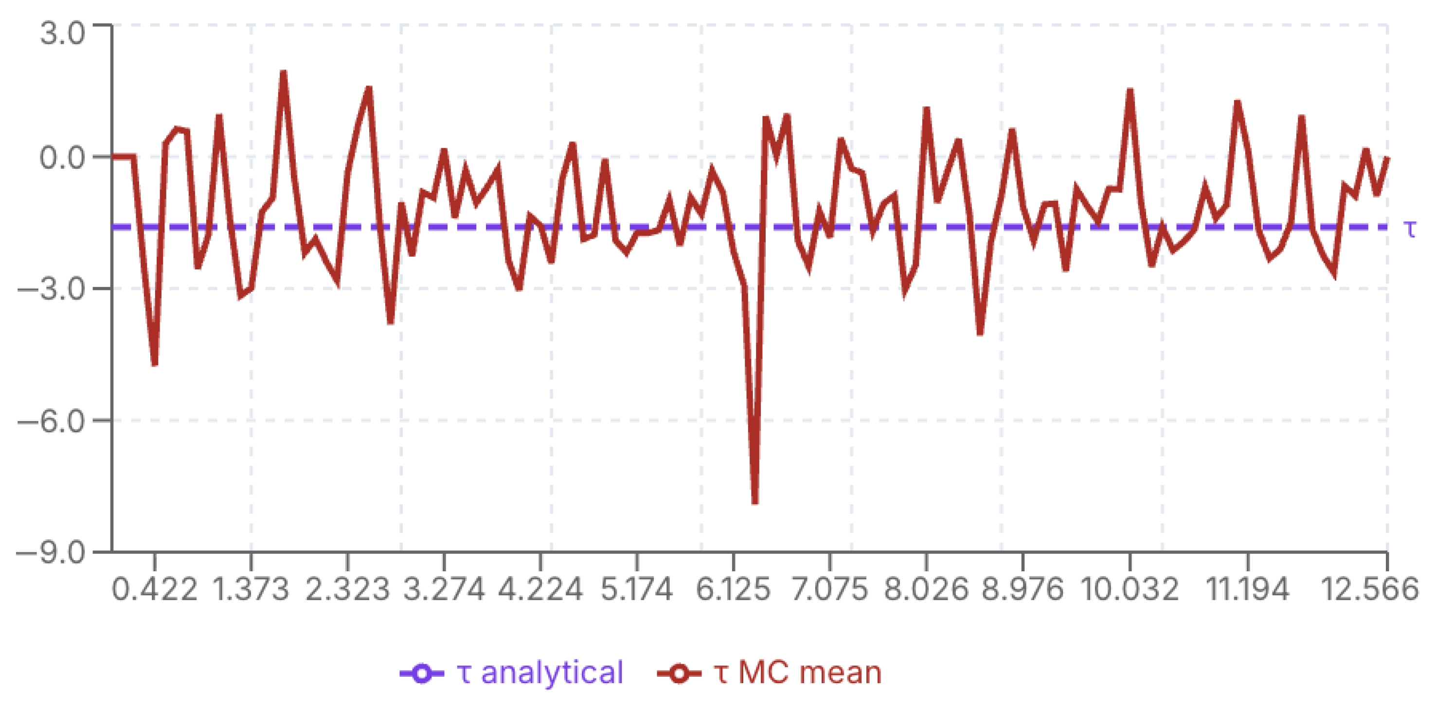
The temporal behavior of curvature and torsion under cubic spline reconstruction is examined through both ensemble-averaged and single-realization perspectives. The Monte Carlo mean at each parameter value t is defined as the pointwise average over all M independent realizations. The ensemble means ${\overline{\kappa }}_{MC}\left(t\right)$ and ${\overline{\tau }}_{MC}\left(t\right)$ are compared against the analytical constants in Figure 8 and Figure 9, respectively.

The MC mean curvature ${\overline{\kappa }}_{MC}\left(t\right)$ exhibits pronounced oscillatory deviations throughout the parameter interval, with values ranging from near zero to approximately 1.80. Near the initial boundary $t\approx 0.317$, the estimated curvature drops sharply toward zero, while near the terminal boundary $t\approx 12.566$ it rises sharply to approximately 1.80. Both effects are direct consequences of the natural spline boundary condition, which forces the second derivative to vanish at the endpoints and thereby distorts the local polynomial coefficients, producing spurious geometric estimates near both domain boundaries. The two boundary-induced effects are opposite in direction but differ in magnitude. Between these boundary-affected regions, the MC mean oscillates around the analytical value with an amplitude of approximately $\pm 0.45$.

The torsion estimate ${\overline{\tau }}_{MC}\left(t\right)$ displays similarly strong fluctuations, with values ranging from approximately $-8$ to above 2. The denominator of the torsion formula, $\parallel {\mathrm{r}}_s^{\prime }\left(t\right)\times {\mathrm{r}}_s^{″}{\left(t\right)\parallel }^2\propto {\kappa }^2{\parallel {\mathrm{r}}_s^{\prime }\parallel }^6$, decreases wherever the estimated curvature is locally reduced, causing the torsion estimate to diverge at such points. As seen in Figure 8, the MC mean curvature exhibits a local depression near $t\approx 6.230$, and this coincident reduction in the curvature-dependent denominator produces the deep negative torsion excursion visible in Figure 9 at the same parameter value.

Despite these local oscillations, the means across the full parameter interval recover the analytical constants

$$\overline{\kappa }=0.8000, \overline{\tau }=-1.6000,$$

(45)

confirming global preservation of geometric characteristics in a statistical sense. However, pointwise reliability is severely limited, as quantified by the single-realization error metrics reported below.

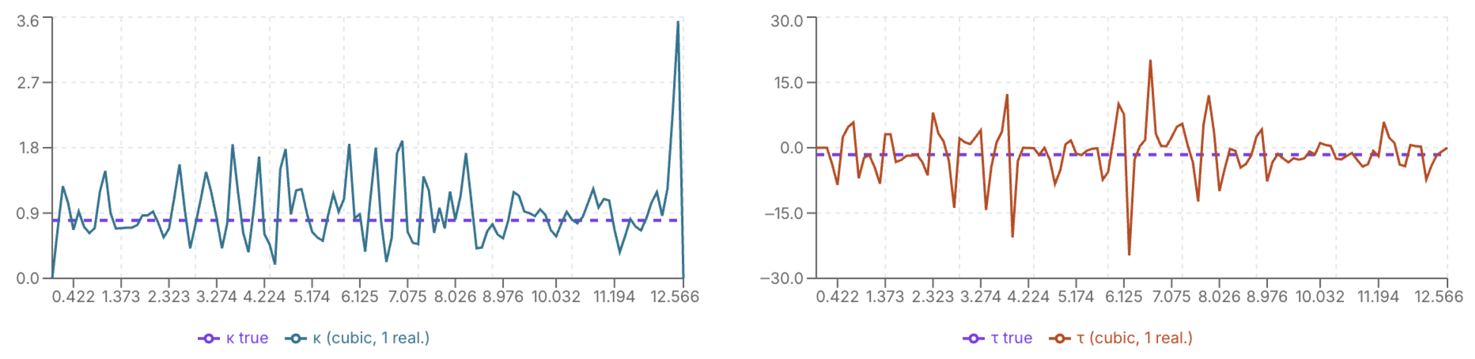
The single-realization estimates ${\kappa }_s\left(t\right)$ and ${\tau }_s\left(t\right)$ are shown in Figure 10. The boundary-induced suppression near $t\approx 0.317$ and amplification near $t\approx 12.566$ reaching approximately $3.6$ are consistent with the MC mean behavior described above. The torsion estimate exhibits a correspondingly large excursion near $t\approx 6.230$, further amplified by the absence of the statistical smoothing provided by ensemble averaging.

The single-realization error metrics are as follows:

$${\mathrm{RMSE}}_{\kappa }=0.4813, {\mathrm{RMSE}}_{\tau }=5.5854,$$

(46)

$${\epsilon }_{\kappa }^{rel}=60.16\%, {\epsilon }_{\tau }^{rel}=349.09\%.$$

(47)

The relative torsion error of $349.09\%$ is nearly six times that of curvature, consistent with the $\mathcal{O}(\sigma /h^3)$ noise amplification established in the Cubic Spline Interpolation section.

The divergence patterns observed in Figure 8 and Figure 9 reflect the stability of Frenet–Serret computations to near-degenerate configurations. When noise-induced perturbations drive $D\left(t\right)=\parallel {\mathrm{r}}^{\prime }\left(t\right)\times {\mathrm{r}}^{″}{\left(t\right)\parallel }^2$ toward zero, as occurs near $t\approx 0.317$ and $t\approx 6.230$, the curvature estimate undergoes local depression, while torsion, computed as $\tau \left(t\right)=det({\mathrm{r}}^{\prime }\left(t\right),{\mathrm{r}}^{″}\left(t\right),{\mathrm{r}}^{‴}\left(t\right))/D\left(t\right)$, exhibits sharp divergence. This behavior is analogous to fold and cusp singularities in singularity theory, where smooth curves develop apparent inflection structures under geometric degeneracy. Although these effects arise as numerical artifacts rather than intrinsic geometric features, they demonstrate that spline-based reconstruction can introduce singularity-like structures under noise, thereby complicating feature detection in applications where Frenet invariants serve as geometric classifiers.

Stability Indices: CSI and TSI

The numerical stability of curvature and torsion is quantitatively evaluated through the Curvature Stability Index (CSI) and the Torsion Stability Index (TSI), defined in Equations (17) and (22), respectively. These indices are analytically derived variance bounds obtained via first-order error propagation applied to the Frenet–Serret formulas under the noise model introduced in the Reference Curve and Frenet–Serret Frame section, and are distinct from the RMSE values in the Behavior of Curvature and Torsion section; RMSE quantifies the error of a single realization, whereas CSI and TSI characterize the expected pointwise variability under the prescribed noise model. The theoretical expressions yield

$$\mathrm{CSI}\left(t\right)={\displaystyle \frac{{\omega }^4}{{({\omega }^2+1)}^3}}·{\sigma }^2=1.2800\times {10}^{-5},$$

(48)

$$\mathrm{TSI}\left(t\right)={cos}^2\left(\omega t\right)·{\displaystyle \frac{{\omega }^4}{{({\omega }^2+1)}^2}}·{\sigma }^2, max\mathrm{TSI}=6.4000\times {10}^{-5}.$$

(49)

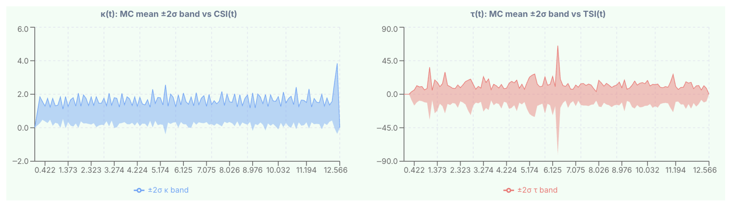
Figure 11 presents the empirical MC variance bands ($\pm 2\sigma$) alongside $\mathrm{CSI}\left(t\right)$ and $\mathrm{TSI}\left(t\right)$.

The $\pm 2\sigma$ confidence band for curvature remains strictly positive throughout the parameter domain, confined to the range [0, ∼4]. The $\pm 2\sigma$ band for torsion is markedly asymmetric; while it generally oscillates within approximately $\pm 45$, it exhibits a pronounced downward spike near $t\approx 6.230$ that reaches approximately $-90$, consistent with the denominator-driven divergence identified in the Behavior of Curvature and Torsion section.

The ratio of the empirical MC variance to the theoretical bound is

$${\displaystyle \frac{{\mathrm{Var}}_{MC}\left[\kappa \right]}{\mathrm{CSI}}}=11,655.3, {\displaystyle \frac{{\mathrm{Var}}_{MC}\left[\tau \right]}{\mathrm{TSI}}}=2,041,794.1.$$

(50)

These ratios of approximately ${10}^4$ for curvature and ${10}^6$ for torsion demonstrate that the linearized noise propagation framework captures only a negligible fraction of the actual estimation variability. The divergence confirms that nonlinear noise propagation effects dominate and that $C^2$ geometric continuity is insufficient to control the statistical behavior of higher-order invariants.

Monte Carlo Stability Analysis

A Monte Carlo simulation with $M=40$ independent realizations was conducted to characterize the statistical distribution of spline-based curvature and torsion estimates. For each parameter value t, the empirical mean is defined as follows:

$${\overline{\kappa }}_{MC}\left(t\right)={\displaystyle \frac{1}{M}}{\displaystyle \sum _{i=1}^M}{\kappa }_i\left(t\right), {\overline{\tau }}_{MC}\left(t\right)={\displaystyle \frac{1}{M}}{\displaystyle \sum _{i=1}^M}{\tau }_i\left(t\right).$$

(51)

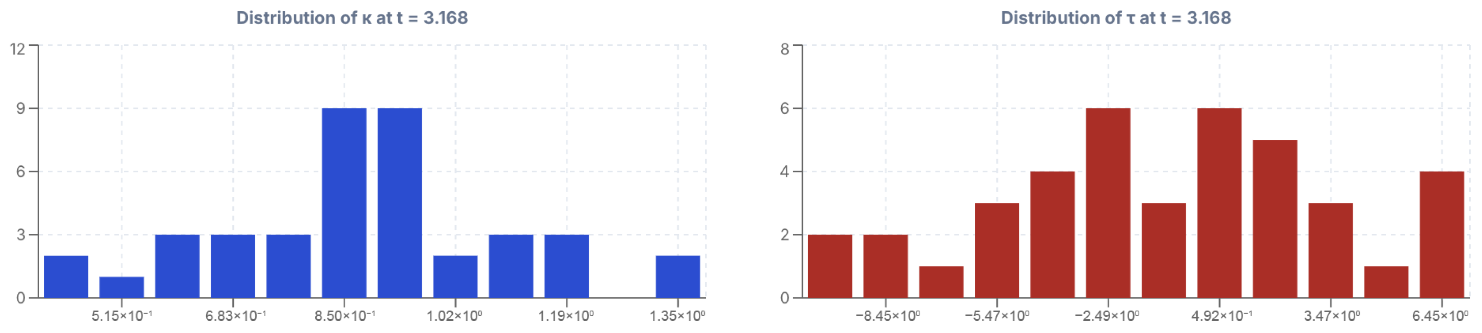
The distributions of $\kappa$ and $\tau$ at the fixed parameter value $t=3.168$, obtained across all M realizations, are presented in Figure 12.

The curvature distribution at $t=3.168$ is right-skewed, with two dominant bins of equal frequency (each with a count of 9) near $0.850$, followed by a gradual tail extending toward $1.35$. The torsion distribution is considerably broader, spanning from approximately $-8.45$ to $6.45$, with the highest bin frequencies observed at approximately $-2.49$ and $0.49$ (each with a count of 6), forming two distinct local peaks. The true value $\tau =-1.6$ falls between these peaks but coincides with neither, indicating a systematic displacement of the empirical distribution relative to the analytical constant. The broader torsion distribution relative to that of curvature is consistent with the higher noise stability of third-order derivatives established in the Cubic Spline Interpolation section.

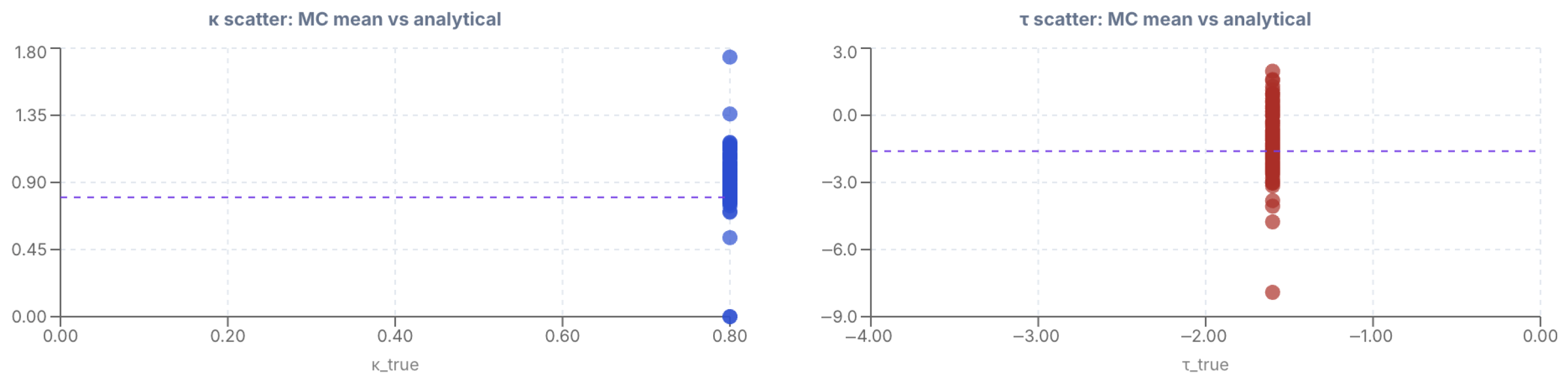
The scatter between MC mean estimates and the true analytical values across all $t\in [0,4\pi ]$ is presented in Figure 13.

Since both ${\kappa }_{\mathrm{true}}$ and ${\tau }_{\mathrm{true}}$ are constants over the parameter domain, the Pearson correlation coefficient is mathematically undefined, and consequently is not reported. The accuracy of the MC mean estimates is assessed through the RMSE values:

$$\mathrm{MC} {\mathrm{RMSE}}_{\kappa }=0.2193, \mathrm{MC} {\mathrm{RMSE}}_{\tau }=1.4351.$$

(52)

In the scatter plots, all estimated values are distributed vertically at the single true value of the respective abscissa. The torsion MC RMSE of 1.4351 is approximately 6.5 times greater than that of the curvature, reflecting the differential noise amplification between second- and third-order derivatives.

Instability Summary

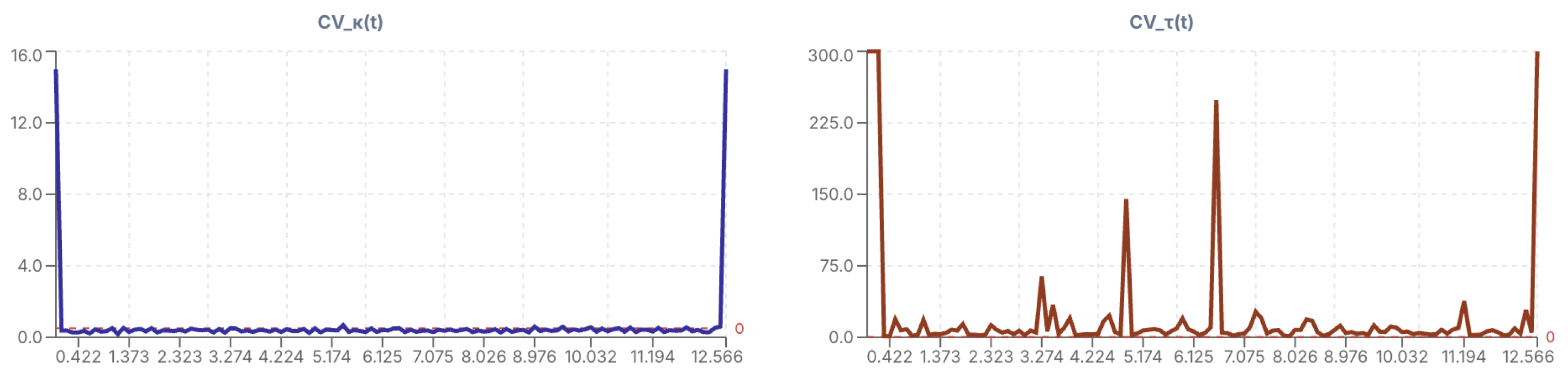
To quantify the spatial extent of numerical instability, the Coefficient of Variation ($\mathrm{CV}$) is adopted as a dimensionless measure of relative dispersion:

$${\mathrm{CV}}_{\kappa }\left(t\right)={\displaystyle \frac{{\sigma }_{\kappa }\left(t\right)}{|{\overline{\kappa }}_{MC}\left(t\right)|}}, {\mathrm{CV}}_{\tau }\left(t\right)={\displaystyle \frac{{\sigma }_{\tau }\left(t\right)}{|{\overline{\tau }}_{MC}\left(t\right)|}}.$$

(53)

A threshold of ${\mathrm{CV}}_{\mathrm{crit}}=0.5$ is adopted, corresponding to a relative standard deviation of 50% with respect to the local mean estimate, above which a point is classified as unstable. The parameter-dependent CV profiles are presented in Figure 14.

The summary statistics are as follows:

$$\mathrm{Mean} {\mathrm{CV}}_{\kappa }=17.0323, \mathrm{Max} {\mathrm{CV}}_{\kappa }=999.0000,$$

(54)

$$\mathrm{Mean} {\mathrm{CV}}_{\tau }=44.0478, \mathrm{Max} {\mathrm{CV}}_{\tau }=999.0000.$$

(55)

The maximum values of 999.0000 represent a numerical cap applied at parameter values where the MC mean approaches zero and the $\mathrm{CV}$ ratio diverges; therefore, the reported mean CV values provide only a lower bound on the true mean instability level across the domain. In the profiles of Figure 14, the plotted curvature CV reaches approximately 16 near the domain boundary and the torsion CV reaches approximately 300 at isolated spike locations, with capped values excluded from the display.

The proportion of unstable points is

$${\displaystyle \frac{N_{\kappa }^{\mathrm{unstable}}}{N_{\mathrm{total}}}}={\displaystyle \frac{17}{120}}=14.2\%, {\displaystyle \frac{N_{\tau }^{\mathrm{unstable}}}{N_{\mathrm{total}}}}={\displaystyle \frac{120}{120}}=100.0\%.$$

(56)

Torsion exhibits an instability ratio of 100%; no evaluation point satisfies the stability criterion. For curvature, 14.2% of points are classified as unstable; these are concentrated at boundary regions and parameter values where the MC mean approaches zero.

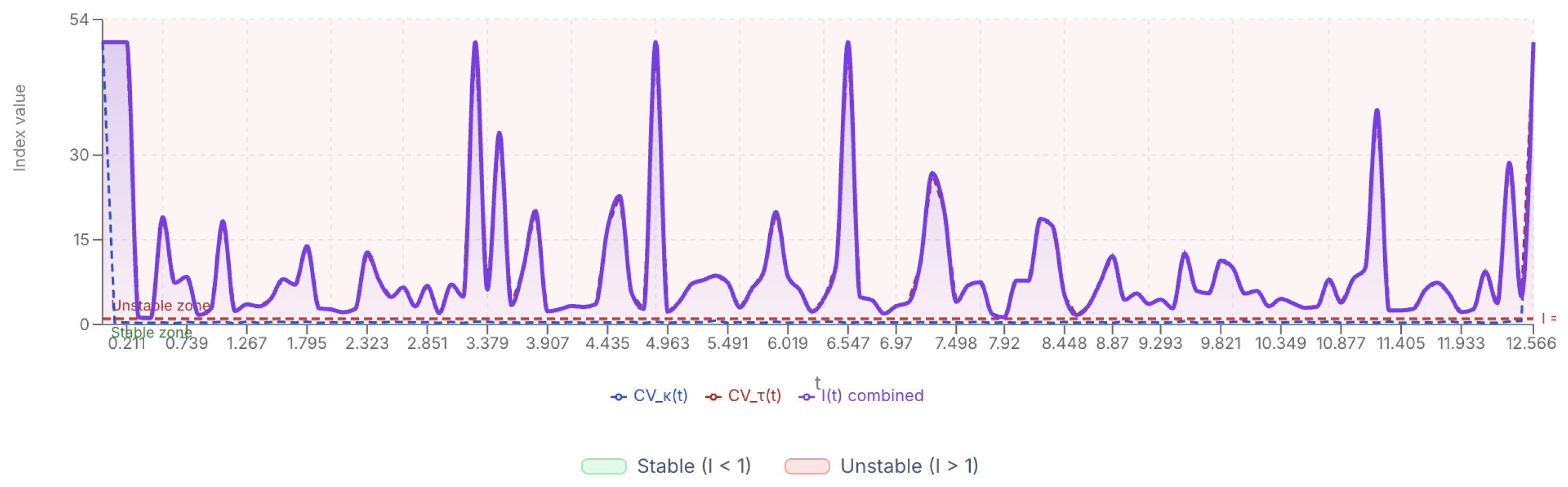
The combined instability index is defined as

$$I\left(t\right)=\sqrt{{\mathrm{CV}}_{\kappa }^2\left(t\right)+{\mathrm{CV}}_{\tau }^2\left(t\right)}.$$

(57)

Its variation over $t\in [0,4\pi ]$ is presented in Figure 15, with display values capped at 50; all summary statistics are computed from the full uncapped values.

$$\mathrm{Mean} I\left(t\right)=50.9605, \mathrm{Max} I\left(t\right)=1412.7993.$$

(58)

The time-averaged individual contributions to $I\left(t\right)$, ${\overline{\Sigma }}_{\kappa }$, and ${\overline{\Sigma }}_{\tau }$, are defined as

$${\overline{\Sigma }}_{\kappa }={\displaystyle \frac{1}{\left|\mathcal{T}\right|}}\sum _{t\in \mathcal{T}}{\mathrm{CV}}_{\kappa }\left(t\right), {\overline{\Sigma }}_{\tau }={\displaystyle \frac{1}{\left|\mathcal{T}\right|}}\sum _{t\in \mathcal{T}}{\mathrm{CV}}_{\tau }\left(t\right),$$

(59)

where $\mathcal{T}$ denotes the subset of evaluation points excluding numerically capped values. The computed values are

$${\overline{\Sigma }}_{\kappa }=0.361, {\overline{\Sigma }}_{\tau }=7.086.$$

(60)

The mean value of $I\left(t\right)=50.96$ exceeds the display cap of 50 because the distribution of $I\left(t\right)$ is strongly right-skewed; the bulk of values lies well below 50, but a small number of large spikes reaching up to 1412.80 pull the uncapped mean above the display threshold. The value ${\overline{\Sigma }}_{\tau }=7.086$ is approximately twenty times larger than ${\overline{\Sigma }}_{\kappa }=0.361$, confirming that torsion is the dominant source of instability across the non-divergent portion of the domain. The peaks in $I\left(t\right)$ coincide with parameter values at which the MC mean of torsion passes through near-zero values. No parameter region consistently satisfies the stability criterion, indicating that the instability is a systemic property of the cubic spline derivative pipeline under noise rather than an artifact confined to isolated regions.

In conclusion, derivative-based differential geometric quantities, in particular torsion, exhibit severe statistical instability under small stochastic perturbations, despite the $C^2$ continuity guaranteed by the cubic spline. These results demonstrate that alternative interpolation strategies with improved derivative stability are necessary for reliable higher-order geometric invariant recovery, motivating the investigation pursued in the subsequent section.

3.2.2. Hermite Interpolation Reconstruction and Monte Carlo-Based Stability Analysis

In this section, the space curve obtained from discrete sample points is reconstructed using the Hermite interpolation method, and the stability of the reconstruction to noise is statistically evaluated. The undisturbed reference curve is taken as a baseline, and the Frenet–Serret frame together with the curvature $\left(\kappa \right)$ and torsion $\left(\tau \right)$ profiles are established. Subsequently, white noise perturbations are added to the sampling points and Hermite-based interpolation is performed. The deviations observed in the resulting $\kappa \left(t\right)$ and $\tau \left(t\right)$ outputs are examined through single realizations, then a Monte Carlo simulation is conducted to analyze the mean behavior, confidence bands, and distributional characteristics under multiple repetitions. In the final stage, error metrics, correlation coefficients, and coefficient of variation-based instability indicators are computed to quantitatively determine the distribution of unstable regions across the parameter domain.

Reference Curve and Frenet–Serret Frame

The reference geometry used for evaluating the Hermite interpolation-based reconstruction is constructed from the undisturbed parametric curve

$$\mathrm{r}\left(t\right)=\left(t,-{\displaystyle \frac{sin\left(\omega t\right)}{{\omega }^2}},-{\displaystyle \frac{cos\left(\omega t\right)}{{\omega }^2}}\right)$$

(61)

with $\omega =2$, defined over the parameter interval $t\in [0,4\pi ]$. The curve is sampled at $N=50$ discrete points. The Frenet–Serret frame vectors $T\left(t\right)$, $N\left(t\right)$, and $B\left(t\right)$ associated with the curve are computed and visualized at selected parameter values, as illustrated in Figure 16. This structure provides the fundamental differential geometric framework that characterizes the directional change and spatial deviation of the curve.

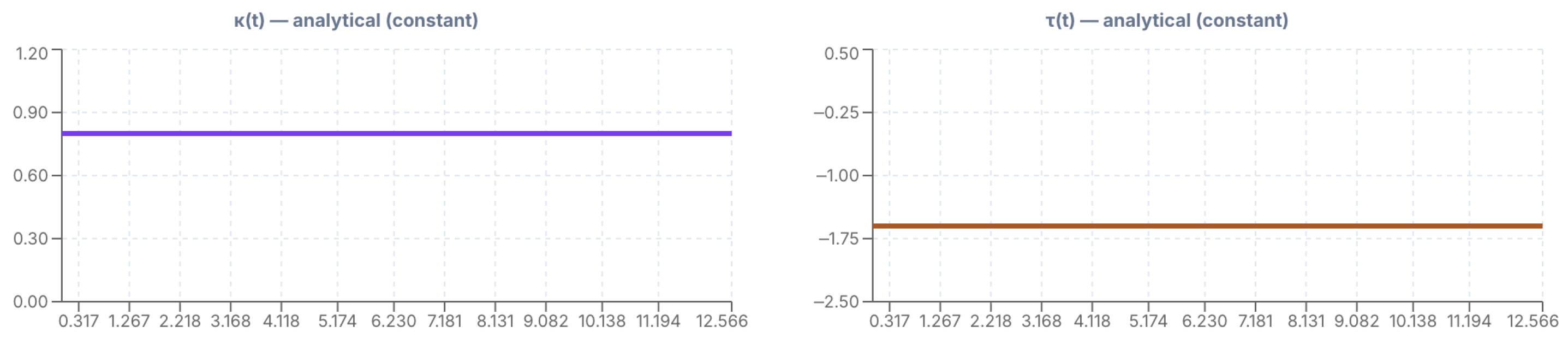
For the reference curve, the curvature $\kappa \left(t\right)$ and torsion $\tau \left(t\right)$ are computed analytically along the parameter domain, and are presented in Figure 17. The resulting profiles confirm that both quantities exhibit stable and uniform behavior across the entire parameter range, with $\kappa \left(t\right)=0.8000$ and $\tau \left(t\right)=-1.6000$ held constant. These baseline values $({\kappa }_{max}=0.8000$, ${ \left|\tau \right|}_{max}=1.6000)$ serve as the analytical references for all subsequent comparisons under Hermite interpolation and noise perturbation.

White Noise Perturbation and Hermite Reconstruction Setup

In order to examine the behavior of the reference curve under noise, zero-mean white Gaussian noise was added to the $N=50$ sampling points. Each coordinate component $(X,Y,Z)$ was perturbed independently, and the standard deviation parameter was selected as $\sigma =0.01$. The resulting noise statistics were computed as ${\mu }_Y=1.926\times {10}^{-3}$, ${\mu }_G=2.470\times {10}^{-3}$, with ${\delta }_Y\approx {\delta }_G\approx 0.00946$, confirming that the imposed perturbations remain approximately centered around zero and are statistically balanced.

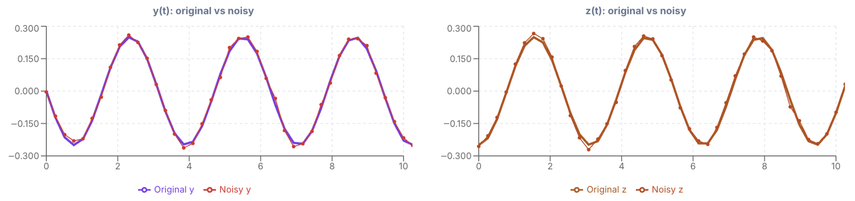
The comparison between the original curve and the noisy discrete samples for the $y\left(t\right)$ and $z\left(t\right)$ components is shown in Figure 18. Using these noisy sample points, Hermite interpolation was applied to obtain a reconstructed parametric curve $\tilde{\mathrm{r}}\left(t\right)$. Although the positional reconstruction remains visually consistent with the original curve, significant deviations arise in the differential geometric quantities (i.e., curvature and torsion) computed from the noisy reconstruction.

Single Hermite Realization: $\kappa$ and $\tau$ Versus Analytical

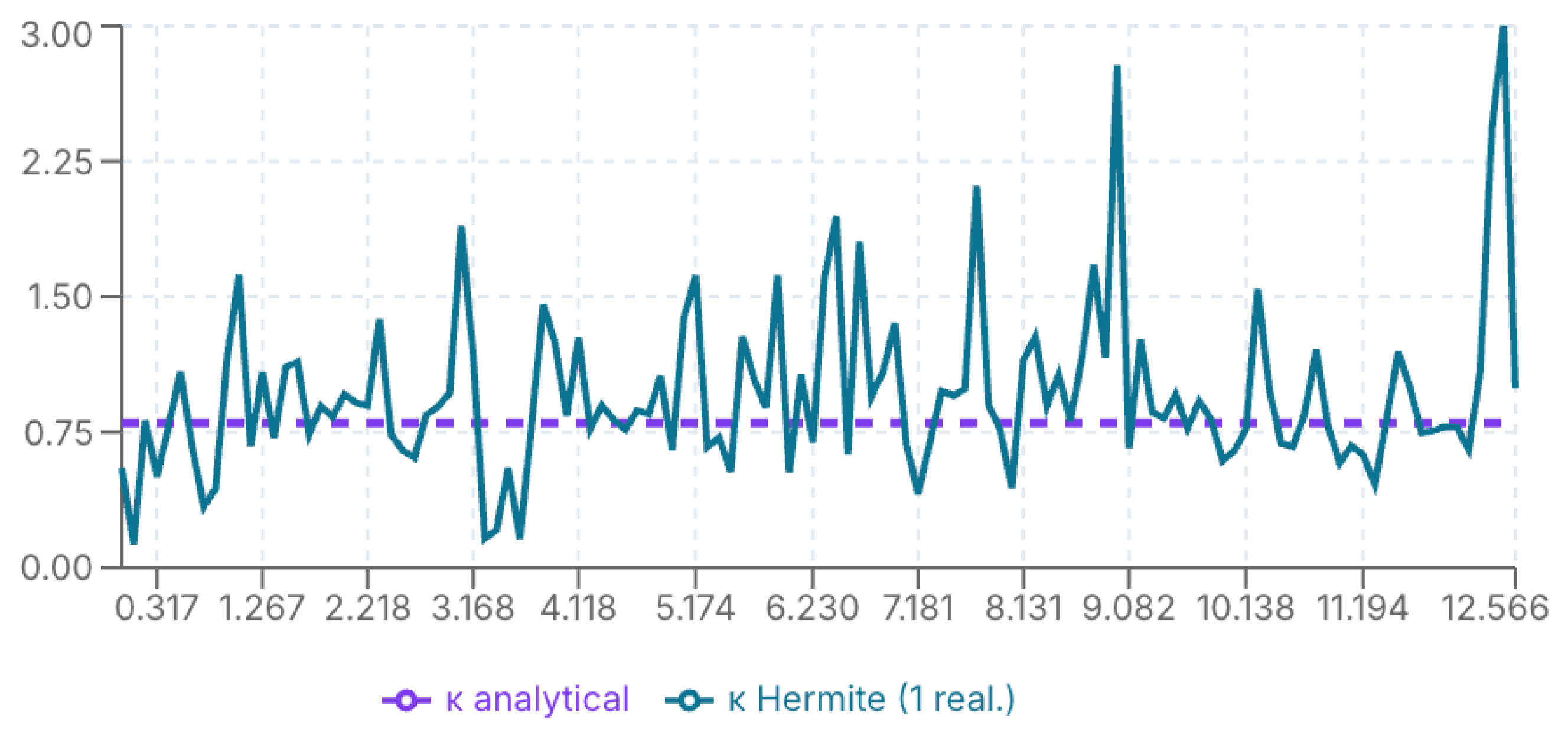
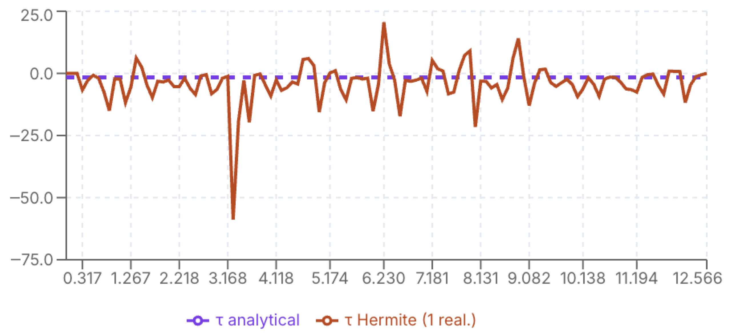
The curvature and torsion computed from a single noisy Hermite spline realization are compared against the analytical reference profiles in Figure 19 and Figure 20.

For curvature, the reconstructed $\kappa \left(t\right)$ fluctuates considerably around the analytical value of $0.8000$, with localized spikes reaching values approaching $3.0$. The single-realization root mean square error for curvature is ${\mathrm{RMSE}}_{\kappa }^{\left(\mathrm{single}\right)}=0.5286$, corresponding to a relative error of $E_{\kappa }^{\mathrm{rel}}=66.07\%$.

For torsion, the deviations are far more pronounced; the reconstructed $\tau \left(t\right)$ exhibits extreme excursions, with ${\mathrm{RMSE}}_{\tau }^{\left(\mathrm{single}\right)}=8.1511$ and $E_{\tau }^{\mathrm{rel}}=509.4\%$. These results demonstrate that although Hermite interpolation provides a geometrically consistent positional reconstruction, differential geometric quantities involving higher-order derivatives exhibit substantial stability even under small-scale noise $(\sigma =0.01)$.

Monte Carlo Stability Analysis

To quantitatively evaluate the statistical behavior of the Hermite reconstructed curve under noise, a Monte Carlo simulation with $M=40$ realizations was performed. For each realization, independent white Gaussian noise with standard deviation $\sigma =0.01$ was added to the $N=50$ sampling points, and the curvature $\kappa \left(t\right)$ and torsion $\tau \left(t\right)$ were recomputed from each noisy dataset. In this way, the mean profiles and $\pm 2\sigma$ confidence bands along the parameter domain were obtained.

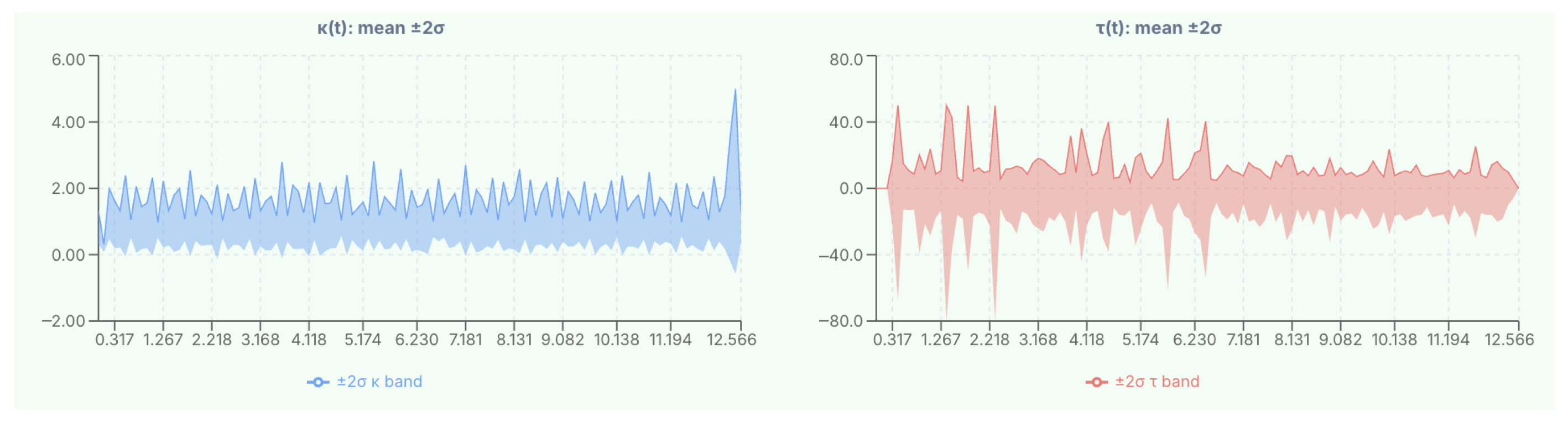
The results are presented in Figure 21. For curvature, the mean profile remains relatively close to the reference value of $0.8000$, while the confidence band exhibits noticeable oscillatory widening along the parameter range. For torsion, the confidence interval is substantially wider, with the band spanning from approximately $-80$ to $+80$ in certain regions. This asymmetry reflects torsion’s higher stability to noise, arising from its dependence on third-order derivatives.

Sample Distributions at Fixed Parameter Value

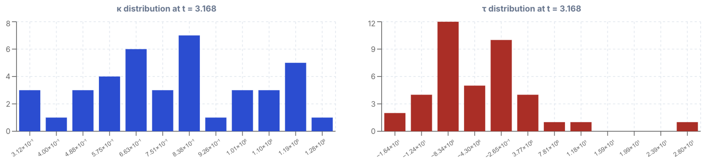
The sample distributions of $\kappa$ and $\tau$ across the $M=40$ Monte Carlo realizations at a representative mid-domain parameter value of $t=3.168$ are shown in Figure 22.

The curvature distribution is concentrated in the range $[3.12\times {10}^{-1}, 1.28]$, centering near the reference value ${\kappa }_{\mathrm{ref}}=0.8000$ with a moderate but non-negligible spread. By contrast, the torsion distribution exhibits a substantially larger variance and asymmetric shape, with values ranging from approximately $-1.64\times {10}^1$ to $+2.80\times {10}^1$. The presence of extreme values and broad dispersion confirms that torsion demonstrates more unstable behavior under noise perturbations.

Reference vs. MC Mean Comparison

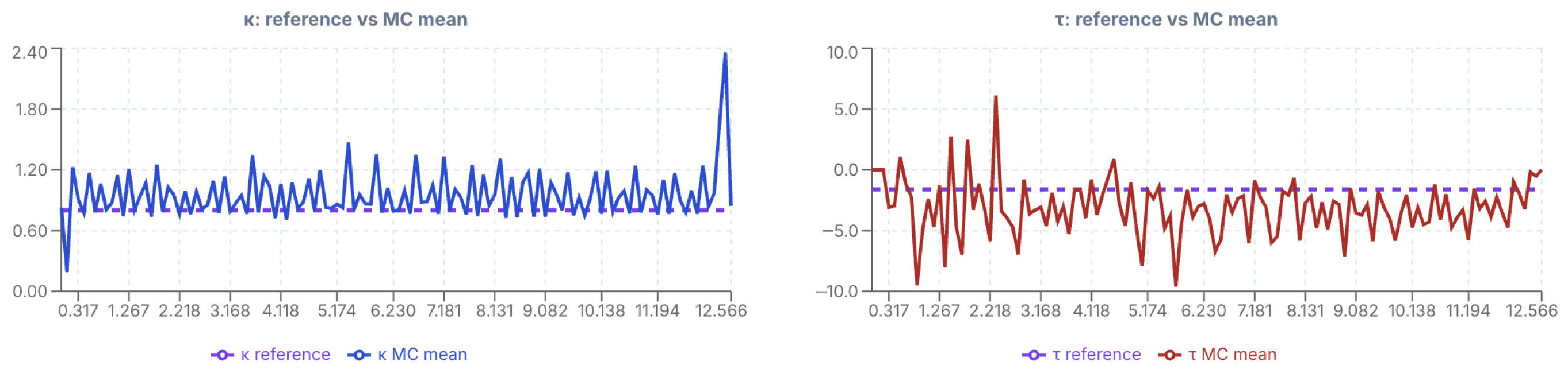
The Monte Carlo mean profiles of curvature and torsion were directly compared with their corresponding analytical reference values, as presented in Figure 23.

For curvature, the MC mean ${\kappa }_{\mathrm{MC},\mathrm{mean}}$ exhibits oscillatory deviations around the reference value ${\kappa }_{\mathrm{ref}}=0.8000$, though the mean trajectory broadly tracks the reference level across most of the parameter domain. For torsion, more pronounced discrepancies appear in certain parameter regions most notably near the interval boundaries and at isolated interior points, with the MC mean ${\tau }_{\mathrm{MC},\mathrm{mean}}$ deviating substantially from the reference value ${\tau }_{\mathrm{ref}}=-1.6000$. These observations clearly reflect the amplifying effect of noise on differential geometric quantities computed through higher-order derivative operations.

Error Analysis: Absolute and Percentage Deviations

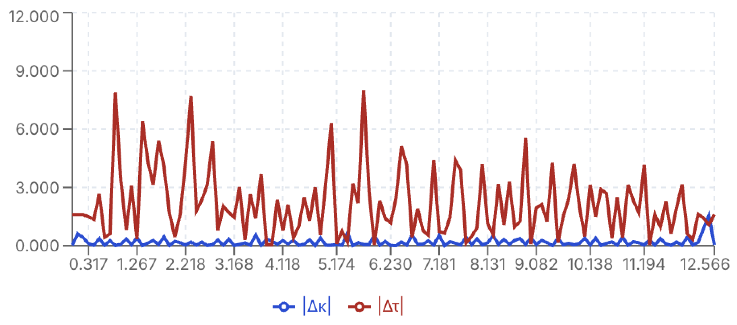
The absolute errors between the Monte Carlo mean profiles and the analytical reference values are defined as

$$|\Delta \kappa \left(t\right)|=|{\kappa }_{\mathrm{MC}}\left(t\right)-{\kappa }_{\mathrm{ref}}\left(t\right)|, |\Delta \tau \left(t\right)|=|{\tau }_{\mathrm{MC}}\left(t\right)-{\tau }_{\mathrm{ref}}\left(t\right)|.$$

(62)

The percentage errors are given by

$${\epsilon }_{\kappa }\left(t\right)=\left({\displaystyle \frac{|\Delta \kappa (t\left)\right|}{|{\kappa }_{\mathrm{ref}}\left(t\right)|}}\right)\times 100, {\epsilon }_{\tau }\left(t\right)=\left({\displaystyle \frac{|\Delta \tau (t\left)\right|}{|{\tau }_{\mathrm{ref}}\left(t\right)|}}\right)\times 100.$$

(63)

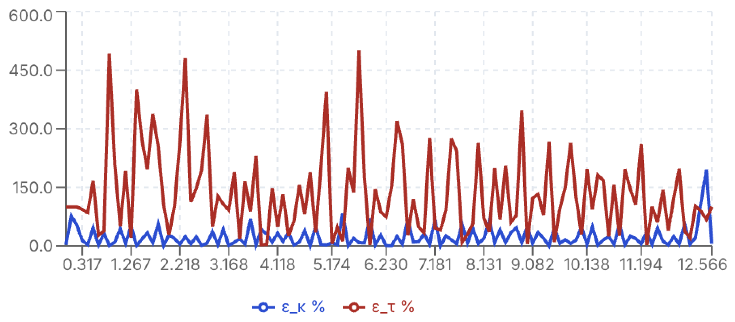
These profiles are presented in Figure 24 and Figure 25. The absolute error for curvature, $|\Delta \kappa (t\left)\right|$, remains comparatively small throughout most of the parameter domain, although localized peaks are observed. For torsion, $|\Delta \tau (t\left)\right|$ reaches values exceeding $8.0$ at multiple locations, with particularly pronounced spikes near specific parameter regions.

The percentage error profiles confirm this disparity: ${\epsilon }_{\kappa }$ remains largely below $100\%$ across the domain, whereas ${\epsilon }_{\tau }$ regularly exceeds $300\%$ and reaches peaks approaching $500\%$ in unstable regions. These findings indicate that despite the relatively small positional deviations produced by Hermite interpolation, the associated differential geometric quantities, particularly torsion, are subject to significant error amplification driven by the propagation of noise through higher-order derivative computations.

Correlation Analysis

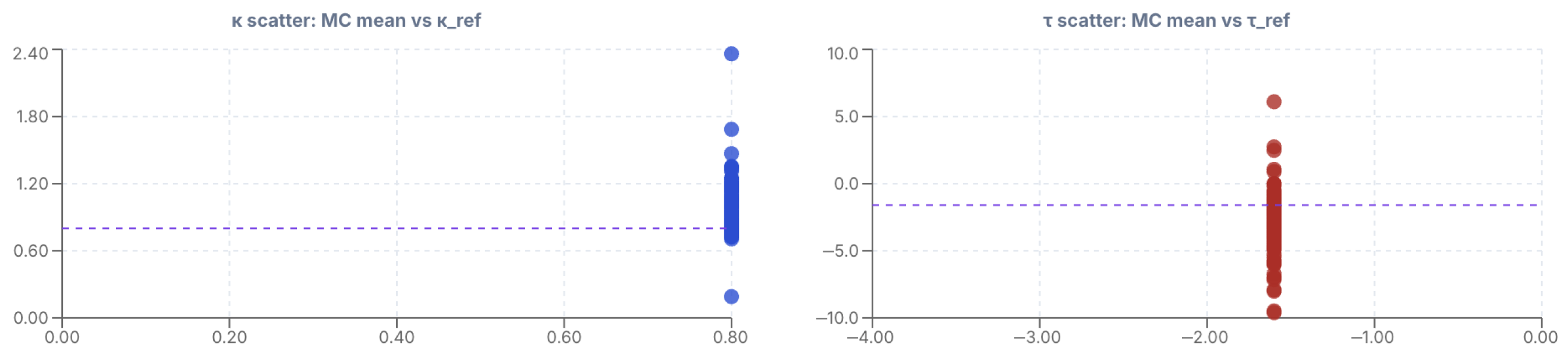
The linear relationship between the Monte Carlo mean values and the reference curvature and torsion profiles was quantitatively assessed using the Pearson correlation coefficient and root mean square error metrics. The scatter plots are presented in Figure 26.

For curvature, ${\kappa }_{\mathrm{MC},\mathrm{mean}}$ values cluster in a narrow vertical band at ${\kappa }_{\mathrm{ref}}=0.80$, while for torsion ${\tau }_{\mathrm{MC},\mathrm{mean}}$ values similarly concentrate near ${\tau }_{\mathrm{ref}}=-1.60$. This vertical alignment arises because the reference curve possesses constant curvature and torsion; consequently, all parameter values project onto a single coordinate in the reference dimension, while the MC mean varies perpendicularly due to noise-induced fluctuations. This geometric configuration precludes the establishment of a meaningful linear correlation.

The Pearson correlation coefficients obtained are $R_{\kappa }\approx 0$ for curvature and $R_{\tau }\approx 0$ for torsion, with corresponding root mean square errors ${\mathrm{RMSE}}_{\kappa }=0.2882$ and ${\mathrm{RMSE}}_{\tau }=2.7588$. The near-zero correlation values reflect the geometric constraint imposed by constant reference values rather than indicating independent variation; in this configuration, the correlation test lacks discriminatory power for assessing reconstruction fidelity.

RMSE Distributions Across Realizations

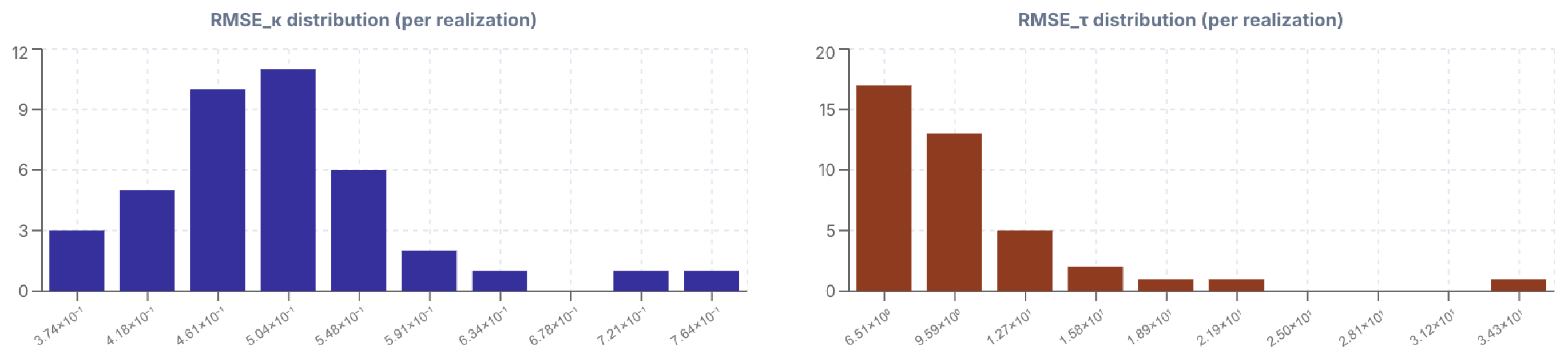
The per-realization ${\mathrm{RMSE}}_{\kappa }$ and ${\mathrm{RMSE}}_{\tau }$ distributions over $M=40$ Monte Carlo repetitions are presented in Figure 27.

For curvature, ${\mathrm{RMSE}}_{\kappa }$ values are concentrated in the range $[3.74\times {10}^{-1}, 7.64\times {10}^{-1}]$, with the distribution exhibiting a moderately symmetric profile; the mean ${\mathrm{RMSE}}_{\kappa }$ across realizations is $0.4992$. For torsion, ${\mathrm{RMSE}}_{\tau }$ values span a wider range from $6.51$ to $3.43\times {10}^1$, with the distribution strongly right-skewed and concentrated near the lower end; the mean ${\mathrm{RMSE}}_{\tau }$ is $10.28$. The substantially larger spread and magnitude of the torsion RMSE distribution relative to curvature corroborates the differential stability of third-order derivative-based quantities to measurement noise.

Variability Analysis and Combined Instability Index

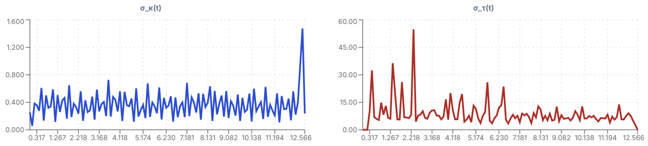
The pointwise standard deviation profiles ${\sigma }_{\kappa }\left(t\right)$ and ${\sigma }_{\tau }\left(t\right)$ computed across $M=40$ Monte Carlo realizations are shown in Figure 28. For curvature, ${\sigma }_{\kappa }\left(t\right)$ exhibits oscillatory behavior with a pronounced increase near the terminal boundary, reaching approximately $1.5$ at $t\approx 12.566$. In contrast, ${\sigma }_{\tau }\left(t\right)$ displays substantially larger fluctuations, with peaks exceeding 55; these are primarily concentrated in the early parameter region $(t<3.5)$. This disparity reflects torsion’s dependence on third-order derivatives, which amplify noise propagation and become particularly sensitive in regions where the denominator $D\left(t\right)$ approaches zero.

To assess relative variability, the Coefficient of Variation (CV) is defined as

$${\mathrm{CV}}_{\kappa }\left(t\right)={\displaystyle \frac{{\sigma }_{\kappa }\left(t\right)}{\left|\kappa \right(t\left)\right|}}, {\mathrm{CV}}_{\tau }\left(t\right)={\displaystyle \frac{{\sigma }_{\tau }\left(t\right)}{\left|\tau \right(t\left)\right|}}.$$

(64)

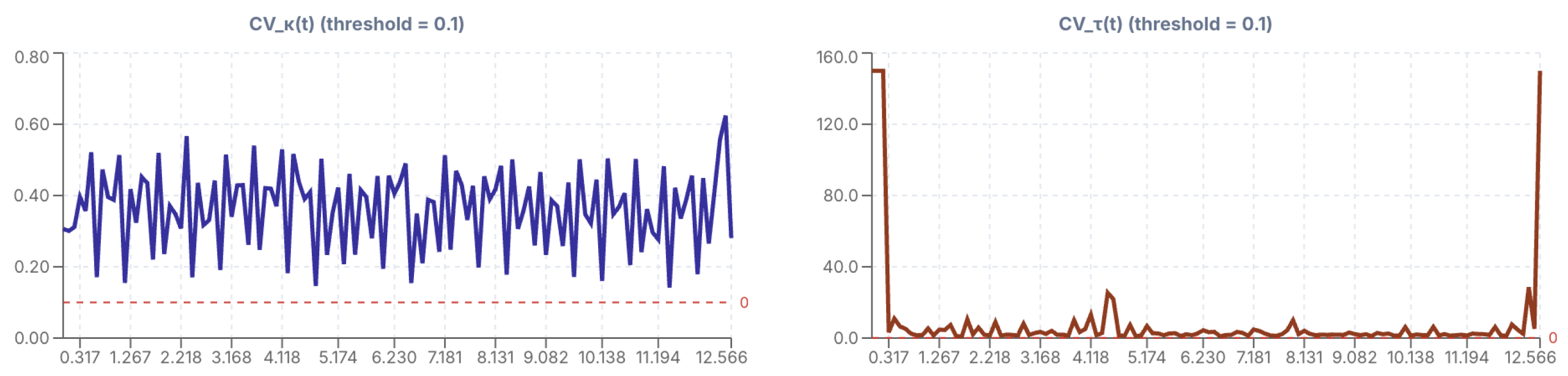
A threshold of ${\mathrm{CV}}_{=}0.1$ is adopted, classifying regions with variability exceeding $10\%$ as unstable. The corresponding profiles are shown in Figure 29. The summary statistics are ${\mathrm{CV}}_{\kappa }^{\mathrm{mean}}=0.3635$, ${\mathrm{CV}}_{\kappa }^{max}=0.6244$, and ${\mathrm{CV}}_{\tau }^{\mathrm{mean}}=36.91$, ${\mathrm{CV}}_{\tau }^{max}=999.0$ (capped for visualization). While ${\mathrm{CV}}_{\kappa }\left(t\right)$ remains within a moderate range, ${\mathrm{CV}}_{\tau }\left(t\right)$ attains very large values at isolated points, notably near $t\approx 0.317$ and $t\approx 12.566$, corresponding to boundary regions and near-degenerate configurations.

Under the noise level $(\sigma =0.01)$, all evaluation points exceed the adopted threshold for both invariants, indicating uniformly elevated variability across the domain under this criterion.

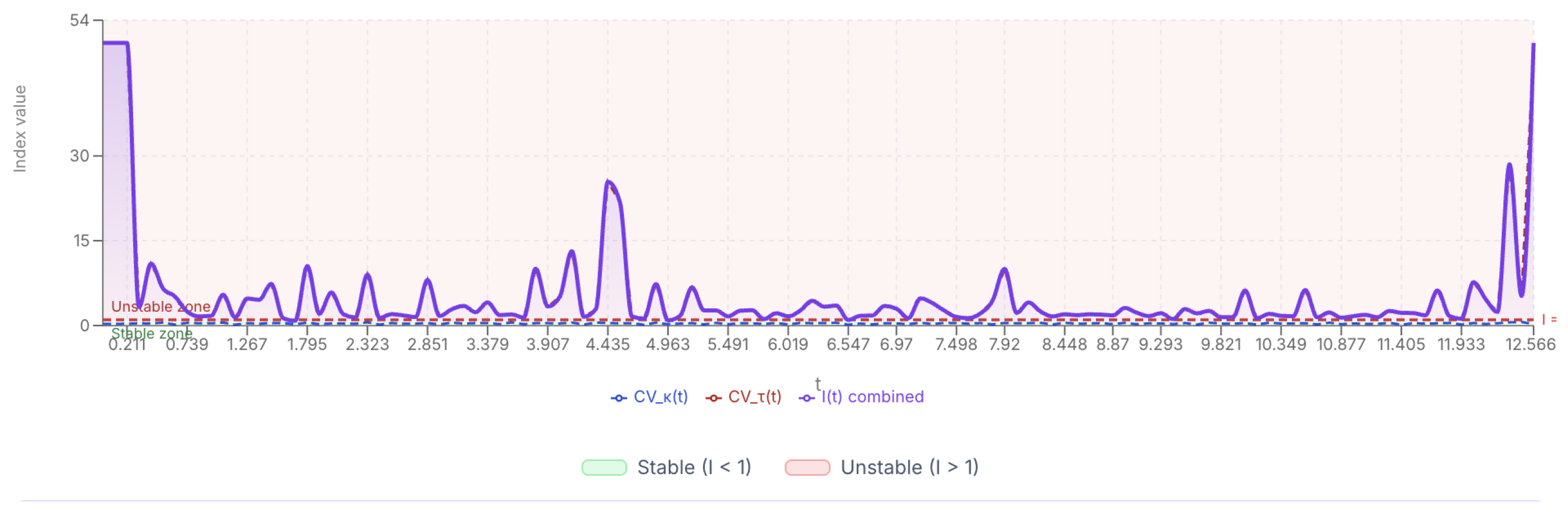
To combine the contributions of curvature and torsion variability, the instability index is defined as

$$I\left(t\right)=\sqrt{{\mathrm{CV}}_{\kappa }^2\left(t\right)+{\mathrm{CV}}_{\tau }^2\left(t\right)}.$$

(65)

The evolution of $I\left(t\right)$ over $t\in [0,4\pi ]$ is shown in Figure 30. The summary values are $I^{\mathrm{mean}}=36.94$ and $I^{max}=999.0$ (capped at 50 for visualization). The corresponding single-realization errors are ${\mathrm{RMSE}}_{\kappa }^{\left(\mathrm{single}\right)}=0.5286$ and ${\mathrm{RMSE}}_{\tau }^{\left(\mathrm{single}\right)}=8.1511$.

The combined index shows that instability is largely governed by the torsion component. Even in regions where curvature variability remains moderate, torsion-driven amplification yields $I\left(t\right)$ values well above unity across most of the domain. The highest values occur near boundary points and previously identified near-degenerate configurations, consistent with the behavior observed in the standard deviation and CV analyses.

From a geometric perspective, this instability is not uniformly distributed, instead being concentrated near regions where the Frenet frame becomes ill-conditioned. In such regions, small perturbations in the reconstructed curve lead to amplified variations in torsion, explaining the observed peaks in both ${\mathrm{CV}}_{\tau }\left(t\right)$ and $I\left(t\right)$.

Overall, the results indicate that while curvature estimates remain relatively stable, torsion is significantly more sensitive to noise. This leads to localized but intense instability regions, highlighting the limitations of Hermite interpolation for applications that rely on higher-order geometric invariants.

These results indicate that the instability is not distributed uniformly but rather concentrated around regions where the Frenet frame becomes ill-conditioned. In particular, when $D\left(t\right)$ approaches zero, small perturbations in the reconstructed curve lead to significant variations in torsion, resulting in the observed peaks in both ${\mathrm{CV}}_{\tau }\left(t\right)$ and $I\left(t\right)$. This behavior explains why torsion-driven instability dominates the combined index and highlights the intrinsic stability of higher-order geometric invariants under noisy interpolation.

3.3. Step 3—Comparative Analysis of Step 1 and Step 2

In this section, the analytical reference solution obtained in Step 1 is systematically compared with the numerical results derived from spline-based reconstruction under noise in Step 2. The overall comparison is summarized in

Table 2. Overall comparison between Step 1 (analytical) and Step 2 (spline-based reconstruction).

Method	$\mathit{\kappa }$ Value	$\mathit{\tau }$ Value	$\mathit{\kappa }$ RMSE	$\mathit{\tau }$ RMSE	$\mathit{\kappa }$ MAE	$\mathit{\tau }$ MAE	$\mathit{\kappa }$ Variance	$\mathit{\tau }$ Variance
Step 1 (Analytical)	0.800000	−1.600000	–	–	–	–	0	0
Step 2—Cubic Spline	0.912413	−1.192509	0.219305	1.435122	0.151856	1.074319	0.149188	65.881889
Step 2—Cubic Hermite Spline	0.957665	−3.122544	0.288191	2.758761	0.189540	2.147665	0.173044	127.202682

.

In Step 1, curvature and torsion are obtained as constant values:

$$\kappa =0.800000, \tau =-1.600000,$$

(66)

with zero variance for both quantities.

In contrast, noticeable deviations are observed in Step 2 under both spline methods. For the cubic spline approach, the computed error measures are

$${\mathrm{RMSE}}_{\kappa }=0.219305, {\mathrm{RMSE}}_{\tau }=1.435122.$$

(67)

For the cubic Hermite spline method, the corresponding values are

$${\mathrm{RMSE}}_{\kappa }=0.288191, {\mathrm{RMSE}}_{\tau }=2.758761.$$

(68)

The variance values further indicate dispersion in the reconstructed invariants. In particular, the torsion variance reaches 65.881889 for the cubic spline method and 127.202682 for the cubic Hermite spline method.

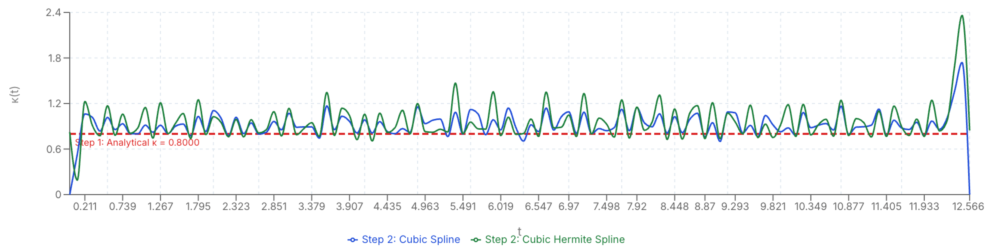
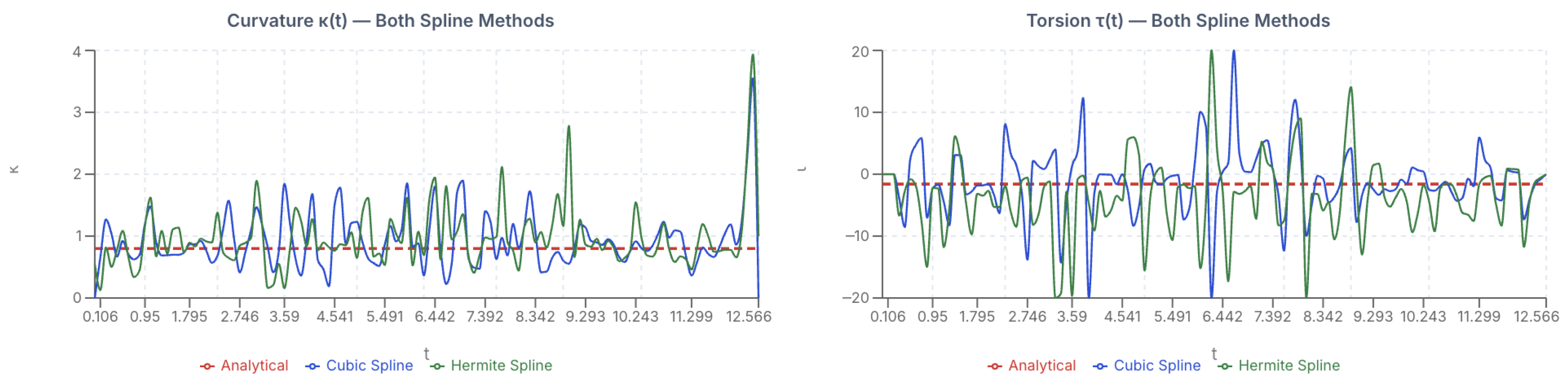
Figure 31 presents the comparison of the curvature profiles. While the analytical solution remains constant at $\kappa =0.8000$, both spline methods produce oscillatory behavior around the reference value.

The cubic spline reconstruction exhibits relatively moderate fluctuations, whereas the cubic Hermite spline shows slightly larger amplitude variations. Despite these deviations, the reconstructed curvature values remain within a limited range around the analytical reference.

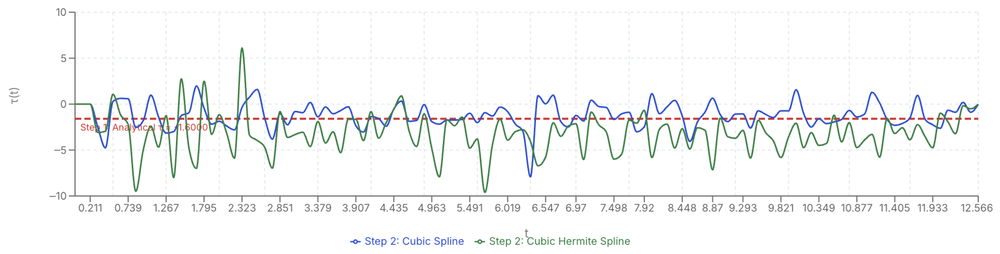
Similarly, Figure 32 shows that torsion exhibits considerably larger amplitude deviations compared to curvature. The analytical torsion value ($\tau =-1.6000$) becomes less distinguishable due to the oscillatory patterns introduced by the spline-based reconstructions.

Both spline methods generate significant fluctuations, with the cubic Hermite spline producing more pronounced deviations. This behavior is consistent with the higher RMSE and variance values reported in Table 2.

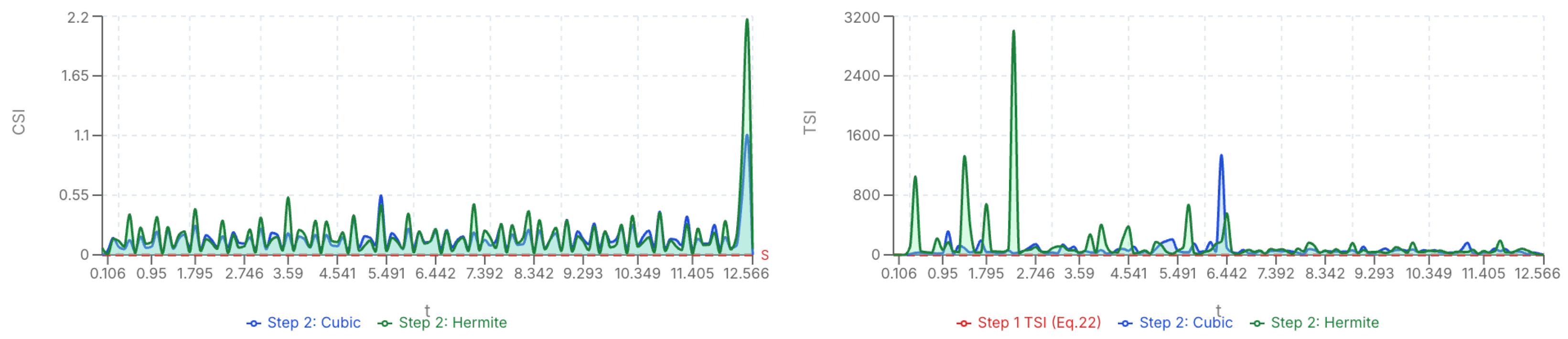
The comparison of CSI and TSI values in Figure 33 provides a quantitative representation of the stability differences between the analytical and numerical stages.

The analytical stability indices remain close to zero, with

$$\mathrm{CSI}=1.2800\times {10}^{-5}, {\mathrm{TSI}}_{max}=6.4000\times {10}^{-5}.$$

(69)

In contrast, the values obtained from spline-based computations are significantly larger, particularly for torsion, indicating increased variability in the numerical reconstruction.

4. Extended Analysis: Geometric Diversity

To assess whether the observed stability patterns arise from the specific choice of constant-invariant geometry or reflect fundamental limitations of spline-based reconstruction, we extend the analysis to two additional reference curves with distinct geometric properties: a variable-curvature helix exhibiting spatially varying Frenet–Serret invariants, and a planar sinusoidal curve with identically zero torsion. All experiments employ the same protocol established in Section 3.2: $N=50$ sampling points, additive noise standard deviation $\sigma =0.01$, and $M=40$ Monte Carlo realizations over the parameter interval $t\in [0,4\pi ]$.

4.1. Variable-Curvature Helix

The variable-curvature helix is defined by the parameterization

$$\mathrm{r}\left(t\right)=\left(cost, sint, {\displaystyle \frac{t^2}{4\pi }}\right), t\in [0,4\pi ].$$

(70)

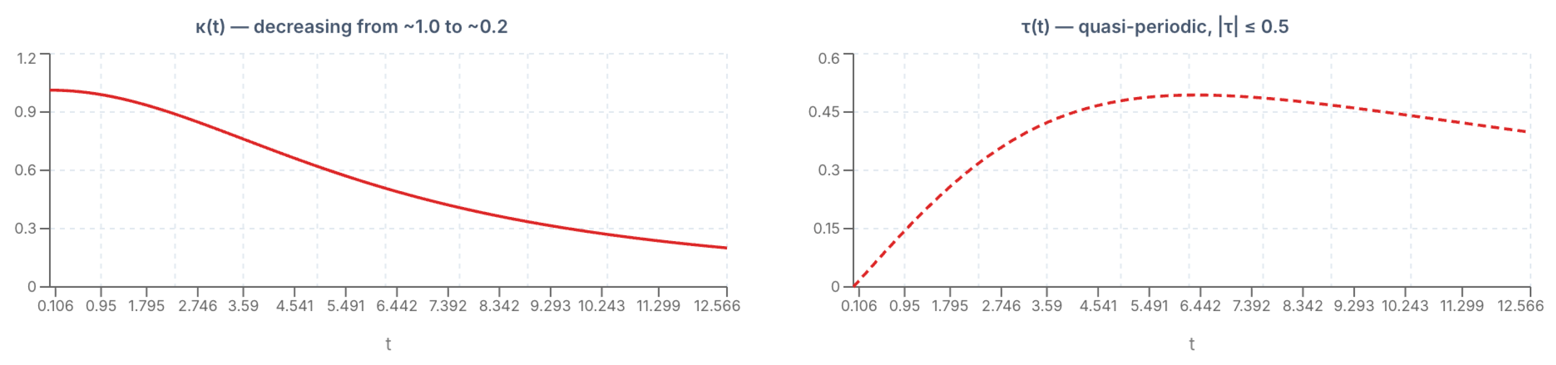
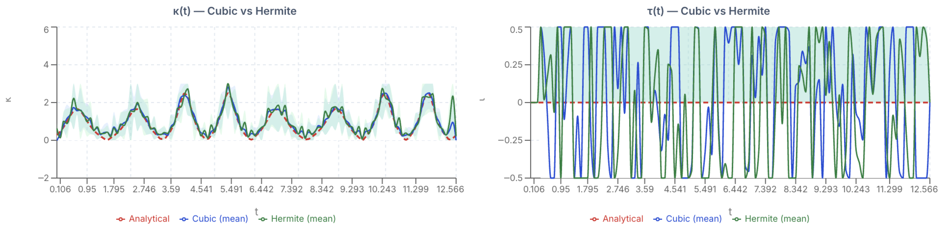
In contrast to the circular helix examined in Section 3.1, this parameterization produces non-constant Frenet–Serret invariants. Application of the formulas derived in Section 2 yields analytical expressions for curvature and torsion as functions of the parameter t. The resulting profiles are presented in Figure 34.

The curvature decreases monotonically from approximately $\kappa \approx 1.01$ at $t=0$ to $\kappa \approx 0.20$ near $t=4\pi$ as the helical structure expands. Torsion exhibits quasi-periodic behavior with amplitude $\left|\tau \right(t\left)\right|\lesssim 0.5$, governed by

$$\tau \left(t\right)={\displaystyle \frac{2\pi t}{1+t^2+4{\pi }^2}},$$

(71)

which reflects the interaction between the circular projection $(cost,sint)$ and the quadratically increasing vertical component $t^2/\left(4\pi \right)$. This geometry more closely resembles analytic signal embeddings of the form $\mathrm{r}\left(t\right)=\left(X\right(t),A(t)sin\varphi (t),g(t\left)\right)$, where temporally varying amplitude and phase produce spatially varying invariants.

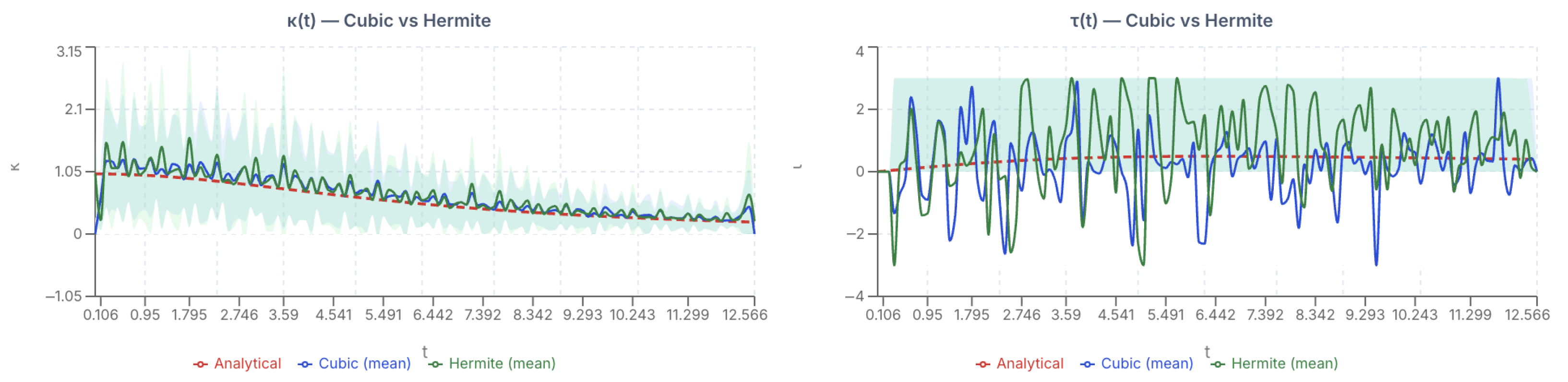
Monte Carlo reconstruction was performed using both cubic spline and cubic Hermite spline interpolation following the procedure established in Section 3.2. Figure 35 presents the ensemble mean estimates alongside $\pm 2\sigma$ confidence bands.

The quantitative error metrics are summarized in

Table 3. Error comparison for variable-curvature helix reconstruction. RMSE and MAE are computed from the Monte Carlo mean over $M=40$ realizations. Bold typeface indicates superior performance.

Metric	Cubic Spline	Hermite Spline	Difference
$\kappa$ RMSE	0.168339	0.197285	0.028946
$\tau$ RMSE	1.114596	1.551472	0.436876
$\kappa$ MAE	0.113317	0.124883	0.011566
$\tau$ MAE	0.791740	1.166018	0.374277
$\kappa$ Variance (mean)	0.085877	0.098349	0.012472
$\tau$ Variance (mean)	53.413035	69.753124	16.340089

.

Despite the variable-invariant geometry, the ratio ${\mathrm{RMSE}}_{\tau }/{\mathrm{RMSE}}_{\kappa }$ remains $6.6$ for cubic spline and $7.9$ for Hermite spline, closely matching the values obtained for the constant helix in Table 2 ($6.5$ and $9.6$, respectively). This consistency across constant and variable regimes indicates that torsion instability is intrinsic to the third-order derivative structure rather than an artifact of uniform geometry. The cubic spline method continues to outperform Hermite interpolation across all metrics, with RMSE reductions of approximately $15\%$ for curvature and $28\%$ for torsion.

4.2. Planar Sinusoidal Curve: Torsion Degeneracy Test

To examine reconstruction behavior under torsion degeneracy, we consider a planar curve with identically zero analytical torsion:

$$\mathrm{r}\left(t\right)=\left(t, 0.5sin(2t+0.3cost), 0\right), t\in [0,4\pi ].$$

(72)

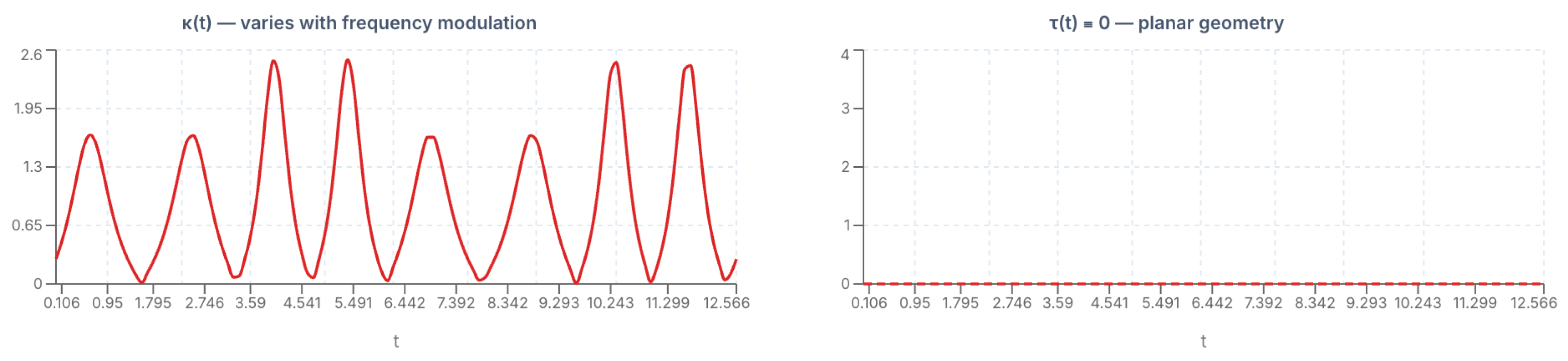
Since the curve lies entirely in the x–y plane, its torsion vanishes by geometric necessity:

$$\tau \left(t\right)\equiv 0 (\mathrm{planar} \mathrm{geometry}).$$

(73)

In contrast, the curvature $\kappa \left(t\right)$ varies continuously due to frequency modulation in the sinusoidal component, as shown in Figure 36.

Under noisy reconstruction, any systematic deviation from $\tau =0$ indicates spurious out-of-plane curvature introduced by numerical artifacts. Such spurious torsion quantifies the extent to which spline-based reconstruction erroneously attributes three-dimensional structure to an intrinsically planar geometry. Figure 37 presents the Monte Carlo results.

Table 4. Planar curve reconstruction: Spurious torsion quantification (${\tau }_{\mathrm{true}}=0$). All non-zero $\tau$ values are spurious noise-induced out-of-plane artifacts from spline differentiation.

Metric	Cubic Spline	Hermite Spline
$\left|\tau \right|$ mean	0.939482	1.328682
$\left|\tau \right|$ max	15.735925	30.772318
$\tau$ RMSE	1.860934	3.276616
$\tau$ Variance	140.476371	309.314844

quantifies the spurious torsion.

The mean spurious torsion ${\left|\tau \right|}_{\mathrm{mean}}\approx 0.94$ for cubic spline and $1.33$ for Hermite spline is approximately two times smaller than the torsion magnitude in the non-planar helical cases ($\left|\tau \right|\approx 1.6$), indicating that the reconstruction methods do not systematically bias the geometry towards non-planarity. However, the variance of torsion estimates remains substantially elevated even under degeneracy. This behavior is a direct consequence of third-order derivative noise amplification, which persists regardless of whether the ground-truth torsion is zero or non-zero. This finding is particularly relevant for analytic signal embeddings with near-planar components, such as slowly varying $g\left(t\right)\approx \mathrm{const}$, where spurious torsion fluctuations may obscure genuine geometric features.

4.3. Cross-Geometry Summary

Table 5. Stability comparison across three geometric regimes. The ratio is defined as ${\mathrm{RMSE}}_{\tau }/{\mathrm{RMSE}}_{\kappa }$. Red bold values indicate cases where the torsion error dominates by a factor greater than 2.

	Cubic Spline			Hermite Spline
Curve Type	$\mathbf{\kappa }$ RMSE	$\mathbf{\tau }$ RMSE	Ratio	$\mathbf{\kappa }$ RMSE	$\mathbf{\tau }$ RMSE	Ratio
Const. Helix ($\tau \ne 0$, const.)	0.219	1.435	6.5	0.288	2.759	9.6
Var. Helix ($\tau \ne 0$, varying)	0.168	1.115	6.6	0.197	1.551	7.9
Planar ($\tau =0$, degeneracy)	0.190	1.861	9.8	0.348	3.277	9.4

consolidates the stability metrics across all three geometric regimes.

The torsion-to-curvature error ratio remains consistently elevated across all three regimes, ranging from 6.5 to 9.8. Notably, the ratio does not collapse in the planar degeneracy case as might be expected; instead, it persists at comparable levels (9.8 for cubic spline and 9.4 for Hermite spline). This result indicates that torsion instability is not merely a consequence of large ground-truth values but arises fundamentally from third-order derivative noise amplification, a structural property of the Frenet–Serret formulation that operates independently of whether $\tau$ is constant, variable, or identically zero.

The consistency of this error hierarchy across constant, variable, and degenerate invariant regimes supports the generalizability of the CSI/TSI framework and its applicability to analytic signal embeddings of the form $\mathrm{r}\left(t\right)=\left(X\right(t),A(t)sin\varphi (t),g(t\left)\right)$, where time-varying amplitude and phase characteristics produce the range of geometric behaviors examined here.

5. Results and Discussion

The numerical results demonstrate that spline-based reconstruction methods preserve the overall geometric structure of the reference curve under the corrected noise level ($\sigma =0.01$). However, the accuracy of the recovered Frenet–Serret invariants is strongly influenced by the derivative order involved in their computation. Curvature, which depends on second-order derivatives, remains relatively stable, whereas torsion, involving third-order derivatives, exhibits significantly higher stability to noise. This behavior is consistently observed across all geometric configurations examined in this study.

Table 6. Cubic spline and cubic Hermite spline error comparison.

Metric	Cubic Spline	Hermite Spline	Difference
$\kappa$ RMSE	0.219305	0.288191>	0.068886
$\tau$ RMSE	1.435122	2.758761	1.323639
$\kappa$ MAE	0.151856	0.189540	0.037684
$\tau$ MAE	1.074319	2.147665	1.073347
$\kappa$ Variance (mean)	0.149188	0.173044	0.023857
$\tau$ Variance (mean)	65.881889	127.202682	61.320792

Note: Bold values indicate the better-performing method for each metric. RMSE and MAE are computed from the Monte Carlo mean ($M=40$ realizations); variance denotes the time-averaged empirical variance.

summarizes the global error metrics obtained for both cubic spline and cubic Hermite spline reconstructions on the constant-invariant circular helix. For curvature, both methods yield comparable results, with the cubic spline achieving slightly lower RMSE and MAE values. Specifically, the curvature RMSE increases from $0.219$ (cubic spline) to $0.288$ (Hermite spline), indicating a modest difference in reconstruction accuracy. This suggests that both interpolation schemes provide a reasonable approximation of the analytical reference at the level of second-order geometric quantities.

In contrast, the difference between the two methods becomes more pronounced in torsion estimation. The torsion RMSE increases from 1.435 for the cubic spline to 2.759 for the Hermite spline, while the corresponding MAE values nearly double. A similar trend is observed in the variance values, where the mean torsion variance rises from 65.9 to 127.2. These results indicate that torsion constitutes the primary source of reconstruction instability and that the Hermite spline is more susceptible to noise amplification in higher-order derivatives. The torsion-to-curvature error ratio of 6.5 for cubic spline and 9.6 for Hermite spline quantifies this differential stability.

Figure 38 presents a direct comparison of $\kappa \left(t\right)$ and $\tau \left(t\right)$ obtained from both spline methods for a representative single realization. In the curvature profile, both methods exhibit oscillations around the analytical reference value $\kappa =0.8$, with deviations remaining within a relatively narrow range. The cubic spline reconstruction follows the reference more closely, while the Hermite spline shows slightly larger fluctuations. The difference becomes more evident in the torsion profile, where the Hermite spline produces wider deviations and more pronounced local excursions around $\tau =-1.6$. These fluctuations reflect the amplification of numerical errors through successive differentiation, compounded by boundary-induced effects inherent to spline reconstruction near the endpoints of the parameter domain.

The extended geometric analysis of Section 4 establishes that the observed stability hierarchy is not specific to the constant-invariant test case but persists across fundamentally different geometric configurations. The torsion-to-curvature error ratio remains consistently elevated, ranging from 6.5 to 9.8 across constant-invariant helices, variable-curvature helices, and planar curves with identically zero torsion. Critically, the ratio does not collapse in the planar degeneracy regime where $\tau \equiv 0$ analytically; instead, it persists at 9.8 for cubic spline and 9.4 for Hermite spline, comparable to non-planar cases. This counterintuitive result confirms that torsion instability arises from structural amplification in third-order derivative computations rather than large ground-truth magnitudes, validating the theoretical predictions of the TSI framework across the full spectrum of invariant behaviors.

The variable curvature helix results (Table 3) demonstrate that the cubic spline maintains superior performance even when invariants vary spatially, achieving RMSE reductions of approximately $15\%$ for curvature and $28\%$ for torsion relative to Hermite interpolation. The planar sinusoidal curve provides a particularly stringent test: although the mean spurious torsion (${\left|\tau \right|}_{\mathrm{mean}}\approx 0.94$ for cubic spline) is approximately half that of helical geometries, the variance of torsion estimates remains substantially elevated, demonstrating that third-order derivative noise amplification operates independently of whether ground-truth torsion is zero or non-zero. This has direct implications for analytic signal embeddings with near-planar components (slowly varying $g\left(t\right)\approx \mathrm{const}$), where distinguishing spurious fluctuations from genuine geometric features becomes critical.

The consistency of the error hierarchy across topologically distinct geometries (three-dimensional helices versus planar curves) and invariant regimes (constant versus variable versus degenerate) establishes the broad applicability of the CSI/TSI framework to signal-derived trajectories of the form $\mathrm{r}\left(t\right)=\left(X\right(t),A(t)sin\varphi (t),g(t\left)\right)$, where temporal variation in amplitude, phase, and vertical components produces the examined range of geometric behaviors. The cross-geometry validation confirms that the observed instability patterns are intrinsic properties of the Frenet–Serret formulation rather than artifacts of specific test configurations.

These observations are in direct agreement with the theoretical stability analysis developed in Section 2. The Curvature Stability Index (CSI) and Torsion Stability Index (TSI) predict that torsion should be more vulnerable to noise due to its dependence on third-order derivatives and the structure of its denominator term. The numerical findings support this prediction: curvature errors remain relatively controlled across all geometric regimes, while torsion displays significantly higher variability in every configuration examined. The additional observation that instability is strongly localized near regions where the Frenet frame becomes degenerate ($D\left(t\right)\to 0$) reveals that instability is intrinsically linked to geometric structure, extending beyond stochastic perturbation effects to encompass denominator-driven amplification and singularity-like behavior. Consequently, although both methods are suitable for positional reconstruction, cubic spline interpolation offers a more reliable framework for the estimation of Frenet–Serret invariants in the presence of noise, particularly when torsion plays a critical role in the application.

6. Conclusions

This study examines the robustness of Frenet–Serret curvature ($\kappa$) and torsion ($\tau$) estimates obtained from noisy discrete curves reconstructed via spline-based interpolation. The comparative performance of cubic spline and cubic Hermite spline methods is evaluated across fundamentally different geometric configurations, with emphasis on the recovery of higher-order geometric invariants under additive noise.

The Curvature Stability Index (CSI) and the Torsion Stability Index (TSI) are employed to analytically characterize perturbation propagation through second- and third-order derivatives. The analysis confirms that torsion is inherently more sensitive to noise than curvature due to its dependence on third-order derivatives. This theoretical prediction is consistently validated by numerical results across all examined geometries, where the torsion formula’s curvature-dependent denominator amplifies local perturbations, leading to larger variability in $\tau$ estimates.

Monte Carlo simulations were performed using three reference curves spanning distinct geometric regimes: a constant-invariant circular helix ($\kappa =0.8$, $\tau =-1.6$), a variable-curvature helix with spatially varying invariants, and a planar sinusoidal curve with identically zero torsion ($\tau \equiv 0$). This diversity validates the framework under constant, variable, and degenerate invariant conditions, directly addressing applicability to analytic signal embeddings $\mathrm{r}\left(t\right)=\left(X\right(t),A(t)sin\varphi (t),g(t\left)\right)$ where temporal variation in amplitude and phase produces the examined range of geometric behaviors. The results yield the following conclusions:

• Cubic spline interpolation produces smoother derivative profiles and more stable geometric estimates across all three regimes, which is due to its global $C^2$ continuity. This method consistently outperforms Hermite interpolation, achieving RMSE reductions of approximately $15\%$ for curvature and $28\%$ for torsion in the variable-curvature case.
• Cubic Hermite spline interpolation exhibits increased stability to perturbations in derivative estimation, particularly in torsion reconstruction, where higher-order derivatives amplify local inconsistencies despite offering local control through tangent specification.
• The torsion-to-curvature error ratio consistently ranges from 6.5 to 9.8 across all geometric regimes. Critically, the ratio does not collapse in the planar regime where $\tau \equiv 0$ analytically, persisting at 9.8 (cubic) and 9.4 (Hermite), which is comparable to non-planar cases.
• This persistence under degeneracy confirms that torsion instability arises from structural amplification in third-order derivative computations rather than from large ground-truth magnitudes. The mean spurious torsion in the planar case (${\left|\tau \right|}_{\mathrm{mean}}\approx 0.94$) is approximately half that of helical geometries, demonstrating no systematic bias toward non-planarity; yet, variance remains substantially elevated, validating the TSI framework across the full spectrum of invariant behaviors.
• The instability is strongly localized near regions where the Frenet frame becomes degenerate ($D\left(t\right)\to 0$), inducing denominator-driven amplification and singularity-like behavior. This reveals that instability is intrinsically linked to geometric structure, extending beyond stochastic perturbation effects.

These findings demonstrate that while both methods provide satisfactory positional reconstruction, their performance diverges for derivative-based quantities. In applications involving noisy discrete data, cubic spline interpolation offers superior reliability for Frenet–Serret invariant estimation, particularly when torsion is critical. The consistency of the error hierarchy across topologically distinct geometries (helices versus planar curves) and invariant regimes (constant, variable, degenerate) establishes the CSI/TSI framework’s broad applicability to signal-derived trajectories. The persistence of torsion instability even under degeneracy has particular relevance for embeddings with near-planar components (slowly varying $g\left(t\right)\approx \mathrm{const}$), where distinguishing spurious fluctuations from genuine features becomes critical.

Future research directions include:

• Applying the framework to experimentally acquired signals under non-Gaussian noise and irregular sampling conditions.
• Investigating hybrid spline approaches combining smoothing and adaptive knot placement to mitigate boundary artifacts and near-degenerate configurations.
• Developing enhanced numerical differentiation schemes for improved stability in regions where $D\left(t\right)\to 0$ induces denominator-driven amplification.
• Exploring CSI and TSI as optimization criteria for adaptive parameter selection in spline-based reconstruction.

In conclusion, this study highlights the fundamental role of derivative order and interpolation smoothness in reliable Frenet–Serret invariant estimation. Ensuring sufficient continuity during reconstruction is essential for controlling noise propagation, particularly in torsion estimation. The validated cross-geometry generalizability of the CSI/TSI framework where error ratios remain elevated regardless of ground-truth magnitudes confirms that torsion instability is an intrinsic property of the Frenet–Serret formulation rather than a configuration-specific artifact, establishing the framework’s applicability to the full parameter space of signal-induced curves.

References

1. do Carmo, M.P. Differential Geometry of Curves and Surfaces; Dover Publications: Mineola, NY, USA, 2016. [Google Scholar]
2. Bruce, J.W.; Giblin, P.J. Curves and Singularities, 2nd ed.; Cambridge University Press: Cambridge, UK, 1992. [Google Scholar]
3. Arnold, J.V.I.; Gusein-Zade, S.M.; Varchenko, A.N. Classification of Critical Points, Caustics and Wave Fronts Singularities of Differentiable Maps; Birkhäuser: Boston, MA, USA, 2012; Volume I. [Google Scholar]
4. Müller, M.; Vaxman, A. Discrete curvature and torsion from cross-ratios. Ann. Mat. Pura Appl. 2021, 200, 1935–1960. [Google Scholar] [CrossRef]
5. Hu, S.; Lundgren, M.; Niemi, A. Discrete Frenet frame, inflection point solitons, and curve visualization with applications to folded proteins. Phys. Rev. E Stat. Nonlinear Soft Matter Phys. 2011, 83, 061908. [Google Scholar]
6. de Boor, C. A Practical Guide to Splines; Springer: New York, NY, USA, 2001. [Google Scholar]
7. Catmull, E.; Rom, R. A class of local interpolating splines. In Computer Aided Geometric Design; Springer: Berlin/Heidelberg, Germany, 1974; pp. 317–326. [Google Scholar]
8. Barnhill, R.E.; Riesenfeld, R.F. Computer Aided Geometric Design; Academic Press: New York, NY, USA, 1974. [Google Scholar]
9. Farin, G. Curves and Surfaces for Computer-Aided Geometric Design: A Practical Guide. In Curves and Surfaces for Computer-Aided Geometric Design: A Practical Guide; Academic Press: Cambridge, MA, USA, 1993. [Google Scholar]
10. Metropolis, N.; Ulam, S. The Monte Carlo method. J. Am. Stat. Assoc. 1949, 44, 335–341. [Google Scholar] [CrossRef] [PubMed]
11. Newman, M.E.J.; Barkema, G.T. Monte Carlo Methods in Statistical Physics. In Monte Carlo Methods in Statistical Physics; Oxford University Press: Oxford, UK, 1999. [Google Scholar]
12. Froggatt, M.; Moore, J. High-spatial-resolution distributed strain measurement in optical fiber with Rayleigh scatter. Appl. Opt. 1998, 37, 1735–1740. [Google Scholar] [CrossRef] [PubMed]
13. Moore, J.P.; Rogge, M.D. Shape sensing using multi-core fiber optic cable and parametric curve solutions. Opt. Exp. 2012, 20, 2967–2973. [Google Scholar] [CrossRef] [PubMed]
14. Wahba, G. Spline Models for Observational Data; SIAM: Philadelphia, PA, USA, 1990. [Google Scholar] [CrossRef]
15. Eubank, R.L. Nonparametric Regression and Spline Smoothing, 2nd ed.; Marcel Dekker: New York, NY, USA, 1999. [Google Scholar]
16. Oehlert, G.W. A note on the delta method. Am. Stat. 1992, 46, 27–29. [Google Scholar] [CrossRef]
Figure 1. Analytical curvature κ ( t ) and torsion τ ( t ) for the reference curve.
Axioms 15 00365 g001
Figure 2. Comparison between the Curvature Stability Index (CSI) and the Torsion Stability Index (TSI) for the reference curve.
Axioms 15 00365 g002
Figure 3. Absolute difference | CSI ( t ) TSI ( t ) | over the parameter interval.
Axioms 15 00365 g003
Figure 4. Transverse components y ( t ) and z ( t ) of the reference curve.
Axioms 15 00365 g004
Figure 5. Three-dimensional helix with Frenet–Serret frame: T (blue), N (red), and B (green) vectors via cavalier oblique projection. The dashed line represents the central axis of the helix, indicating the propagation direction and providing a geometric reference for the oblique projection.
Axioms 15 00365 g005
Figure 6. Noisy discrete samples and cubic spline reconstruction: y ( t ) component.
Axioms 15 00365 g006
Figure 7. Component-wise comparison: y ( t ) (left panel) and z ( t ) (right panel) original vs. noisy.
Axioms 15 00365 g007
Figure 8. κ ( t ) : Monte Carlo mean vs. analytical value (cubic spline).
Axioms 15 00365 g008
Figure 9. τ ( t ) : Monte Carlo mean vs. analytical value (cubic spline).
Axioms 15 00365 g009
Figure 10. κ ( t ) and τ ( t ) from a single cubic spline realization vs. analytical values.
Axioms 15 00365 g010
Figure 11. CSI vs. Var M C [ κ ] and TSI vs. Var M C [ τ ] with ± 2 σ confidence bands.
Axioms 15 00365 g011
Figure 12. Distributions of Monte Carlo κ and τ samples at t = 3.168 .
Axioms 15 00365 g012
Figure 13. Scatter plot of MC mean estimates vs. analytical values for curvature and torsion. The dashed horizontal lines indicate the analytical reference values κ true = 0.8 and τ true = 1.6 , respectively.
Axioms 15 00365 g013
Figure 14. CV κ ( t ) and CV τ ( t ) : Coefficient of variation profiles with instability threshold CV crit = 0.5 .
Axioms 15 00365 g014
Figure 15. I ( t ) = CV κ 2 + CV τ 2 : Combined instability index over t [ 0 , 4 π ] ; green = stable ( I < 1 ), red = unstable ( I > 1 ). Values are capped at 50 for display clarity.
Axioms 15 00365 g015
Figure 16. Three-dimensional helix with Frenet–Serret frame T (tangent, blue), N (normal, red), and B (binormal, green) vectors. Hermite reconstruction of the parametric curve r ( t ) = t , sin ( ω t ) / ω 2 , cos ( ω t ) / ω 2 with ω = 2 , t [ 0 , 4 π ] , sampled at N = 50 discrete points. The dashed line represents the central axis of the helix, indicating the propagation direction and providing a geometric reference for the oblique projection.
Axioms 15 00365 g016
Figure 17. Curvature κ ( t ) and torsion τ ( t ) analytical profiles of the reference curve. κ ( t ) = 0.8000 and τ ( t ) = 1.6000 constant analytical reference baseline. The constant profiles confirm the uniform helical structure used as the reference.
Axioms 15 00365 g017
Figure 18. Original curve vs. noisy discrete samples for the y ( t ) and z ( t ) components. Noise parameters: μ Y = 1.926 × 10 3 , μ G = 2.470 × 10 3 , δ Y δ G 0.00946 . The imposed perturbations remain approximately centered around zero and are statistically balanced.
Axioms 15 00365 g018
Figure 19. κ ( t ) : Single Hermite spline realization versus analytical profile. The reconstructed curvature fluctuates considerably around the analytical value κ = 0.8000 , with RMSE κ ( single ) = 0.5286 and relative error E κ rel = 66.07 % .
Axioms 15 00365 g019
Figure 20. τ ( t ) : Single Hermite spline realization versus analytical profile. The reconstructed torsion exhibits extreme excursions, with RMSE τ ( single ) = 8.1511 and relative error E τ rel = 509.4 % .
Axioms 15 00365 g020
Figure 21. Monte Carlo mean ± 2 σ confidence intervals for κ ( t ) and τ ( t ) with M = 40 realizations. The curvature mean profile remains close to the reference value with moderate oscillations while the torsion confidence interval is substantially wider, reflecting torsion’s higher stability to noise, arising from its third-order derivative dependence.
Axioms 15 00365 g021
Figure 22. Histograms of MC κ and τ samples at fixed t = 3.168 distribution over M realizations. The curvature distribution centers near κ ref = 0.8000 with moderate spread, while the torsion distribution exhibits substantially larger variance and asymmetric shape, confirming unstable behavior under noise.
Axioms 15 00365 g022
Figure 23. κ ref vs. κ MC , mean and τ ref vs. τ MC , mean over the full parameter domain. For curvature, the MC mean exhibits oscillatory deviations around the reference value, whereas torsion shows more pronounced discrepancies, reflecting the amplifying effect of noise on higher-order derivatives.
Axioms 15 00365 g023
Figure 24. | Δ κ ( t ) | and | Δ τ ( t ) | absolute MC mean errors. The curvature error remains comparatively small across most of the domain, while torsion errors reach substantially larger values at multiple locations.
Axioms 15 00365 g024
Figure 25. ε κ ( t ) and ε τ ( t ) percentage errors (%). The curvature percentage error remains largely below 100 % , whereas torsion errors regularly exceed 300 % and approach 500 % in unstable regions.
Axioms 15 00365 g025
Figure 26. Scatter plots: κ MC , mean vs. κ ref and τ MC , mean vs. τ ref across t [ 0 , 4 π ] . The vertical clustering patterns arise from the constant reference geometry. R κ 0 , R τ 0 , RMSE κ = 0.2882 , RMSE τ = 2.7588 .
Axioms 15 00365 g026
Figure 27. Per-realization RMSE κ and RMSE τ distributions over M = 40 realizations. Curvature RMSE values exhibit moderate spread (mean RMSE κ = 0.4992 ), while torsion RMSE values show substantially larger spread and magnitude (mean RMSE τ = 10.28 ), confirming its higher stability to noise.
Axioms 15 00365 g027
Figure 28. σ κ ( t ) and σ τ ( t ) pointwise standard deviation over Monte Carlo realizations. The larger variations in σ τ ( t ) reflect the amplification of noise through higher-order derivatives and denominator stability.
Axioms 15 00365 g028
Figure 29. CV κ ( t ) and CV τ ( t ) with instability threshold = 0.1 . Curvature remains comparatively stable, while torsion exhibits large localized peaks.
Axioms 15 00365 g029
Figure 30. Combined instability index I ( t ) over t [ 0 , 4 π ] . Higher values indicate increased instability, primarily driven by torsion variability.
Axioms 15 00365 g030
Figure 31. Comparison of curvature κ ( t ) between the analytical reference and spline-based reconstructions.
Axioms 15 00365 g031
Figure 32. Comparison of torsion τ ( t ) between the analytical reference and spline-based reconstructions.
Axioms 15 00365 g032
Figure 33. Comparison of CSI and TSI values between analytical and spline-based computations.
Axioms 15 00365 g033
Figure 34. Analytical curvature and torsion profiles for the variable-curvature helix r ( t ) = ( cos t , sin t , t 2 / ( 4 π ) ) . Left: The Curvature κ ( t ) decreases monotonically from approximately 1.0 to 0.2 as the helix expands. Right: The torsion τ ( t ) exhibits quasi-periodic oscillations with amplitude | τ | 0.5 , reflecting the interplay between the circular projection and quadratically increasing vertical component.
Axioms 15 00365 g034
Figure 35. Monte Carlo reconstruction of the variable-curvature helix using cubic spline and Hermite spline with N = 50 , σ = 0.01 , and M = 40 . Mean trajectories are shown with ± 2 σ confidence bands. The dashed reference curve indicates the analytical solution. Left: Curvature κ ( t ) . Right: Torsion τ ( t ) . Both methods exhibit elevated variance in torsion relative to curvature, consistent with the findings in Section 3.2.
Axioms 15 00365 g035
Figure 36. Planar sinusoidal curve: The curvature κ ( t ) varies, whereas the torsion satisfies τ ( t ) 0 analytically. Therefore, any reconstructed τ 0 constitutes a spurious artifact caused by noise-induced out-of-plane effects.
Axioms 15 00365 g036
Figure 37. Spurious torsion under noise: Cubic spline vs. Hermite spline. Both methods oscillate around τ = 0 , with Hermite exhibiting wider variance. Left: The curvature reconstruction remains stable. Right: The torsion exhibits elevated variance despite zero ground truth.
Axioms 15 00365 g037
Figure 38. Direct comparison of curvature and torsion obtained via cubic spline (blue) and cubic Hermite spline (green) under noisy conditions ( σ = 0.01 ). The dashed red line represents the analytical reference. Torsion values are displayed within the capped range ± 20 for clarity.
Axioms 15 00365 g038