Convergence Analysis of Wang–Zheng-Type Iterative Methods for the Simultaneous Approximation of Multiple Zeros

Abstract

This paper studies a new family of iterative methods for the simultaneous approximation of polynomial zeros with known multiplicities. The methods are obtained by combining the Wang–Zheng iteration function with an arbitrary iteration function. This approach leads to a class of methods referred to as Wang–Zheng-type methods with correction for multiple zeros. A local convergence analysis is developed for a wide class of iteration functions. The analysis describes the conditions under which the proposed methods converge locally. Several known iterative methods are examined as special cases of the general results. In particular, the family constructed by Kyurkchiev and Andreev (1990) is included. For every positive integer N, the N-th method of this family has convergence order $3N+1$. The main local convergence theorem extends, complements and improves earlier results by Wang and Wu (1987) and by Kyurkchiev and Andreev (1990).

1. Introduction

One of the classical problems in numerical analysis is the computation of polynomial zeros. Many iterative methods have been proposed and extensively studied for the case of simple zeros. However, the situation is significantly more difficult when multiple zeros are involved. The construction of efficient iterative methods with high convergence order for multiple zeros remains a challenging and less explored problem in the literature.

One approach to constructing simultaneous methods with accelerated convergence is to combine a well-known iteration function with an arbitrary one. In this paper, we use the Wang–Zheng-type iteration function [1] in the case of multiple zeros with known multiplicities. This approach has been considered in several related works [2,3,4,5,6,7].

Let $f\in \mathbb{C}\left[z\right]$ be a polynomial of degree $n\ge 2$ and let ${\xi }_1,\dots ,{\xi }_s$ with $s\ge 2$ be all distinct zeros of f with multiplicity $m_1,\dots ,m_s$, respectively, $(m_1+\dots +m_s=n)$. The case $s=1$ is trivial and will not be considered.

Definition 1 

(Wang–Zheng-type method with correction for multiple zeros). Let $f\in \mathbb{C}\left[z\right]$ be a polynomial of degree $n\ge 2$ and let

$$\Phi : \mathcal{D}\subset {\mathbb{C}}^s\to {\mathbb{C}}^s$$

be an iteration function. Define the following iterative method:

$$x^{(k+1)}=T\left(x^{\left(k\right)}\right),k=0,1,2,\dots ,$$

(1)

where the iteration function $T: D\subset {\mathbb{C}}^s\to {\mathbb{C}}^s$ is defined by

$$T_i\left(x\right)=\left\{\begin{array}{cc}{x}_i-m_i{Z}_i{\left(x\right)}^{-1}\hfill & \mathit{if}f\left(x_i\right)\ne 0,\hfill \\ x_i\hfill & \mathit{if}f\left(x_i\right)=0,\hfill \end{array}\right.$$

(2)

with

$$Z_i\left(x\right)={\displaystyle \frac{1+m_i}{2}}{\displaystyle \frac{f^{\prime }\left(x_i\right)}{f\left(x_i\right)}}-{\displaystyle \frac{m_i}{2}}{\displaystyle \frac{f^{″}\left(x_i\right)}{f^{\prime }\left(x_i\right)}}-{\displaystyle \frac{f\left(x_i\right)}{2f^{\prime }\left(x_i\right)}}\left({\left(\sum _{j\ne i}{\displaystyle \frac{m_j}{x_i-{\Phi }_j\left(x\right)}}\right)}^2+m_i\sum _{j\ne i}{\displaystyle \frac{m_j}{{(x_i-{\Phi }_j\left(x\right))}^2}}\right)$$

and the domain of T is the set

$$D=\{x\in \mathcal{D}: x_i\ne {\Phi }_j\left(x\right)\mathit{for}j\ne i,f^{\prime }\left(x_i\right)\ne 0\mathit{and}{Z}_i\left(x\right)\ne 0\mathit{whenever}f\left(x_i\right)\ne 0\}.$$

(3)

The aim of this paper is to provide a complete local convergence analysis of the newly proposed Wang–Zheng-type method with correction for multiple zeros. In Section 2, we prove the main theorem, which establishes sufficient conditions together with a priori and a posteriori error estimates. These estimates guarantee the Q-convergence of the iterative process. Section 3 discusses several special cases. Corollary 1 shows that our main result (Theorem 1) extends, supplements, and improves the result of Wang and Wu (Theorem 2). We consider the method with corrections of well-known methods such as Newton’s, Halley’s, and Chebyshev-like. Section 4 examines the family of Kyurkchiev and Andreev with order of convergence $3N+1$. Furthermore, our main theorem extends and improves the corresponding result of Kyurkchiev and Andreev (Theorem 3). Section 5 ends this paper with some numerical experiments.

2. Main Result

Let us recall some notations. Vector space ${\mathbb{C}}^s$ is endowed with a p-norm ${\parallel ·\parallel }_p: {\mathbb{C}}^s\to \mathbb{R}$ defined by

$${\parallel x\parallel }_p={\left(\sum _{i=1}^s{\left|x_i\right|}^p\right)}^{1/p}\mathrm{for}\mathrm{some}1\le p\le \infty .$$

Also, define in ${\mathbb{C}}^s$ a cone norm $\parallel ·\parallel : {\mathbb{C}}^s\to {\mathbb{R}}^s$ by

$$\parallel x\parallel =\left(\right|x_1|,\dots ,|x_s\left|\right),$$

as the real vector space ${\mathbb{R}}^s$ is endowed with coordinate-wise partial ordering defined by

$$x⪯y\mathrm{if}\mathrm{and}\mathrm{only}\mathrm{if}{x}_i\le y_i\mathrm{for}\mathrm{each}i=1,\dots ,s.$$

For the sake of brevity, we define the quantities $a=a(p,m_1,\dots ,m_s)$ and $b=b\left(p\right)$ as follows:

$$a=\underset{1\le i\le s}{\max }{\displaystyle \frac{1}{m_i}}{\left(\sum _{j\ne i}{m}_j^q\right)}^{1/q}\mathrm{and}b=2^{1/q},$$

(4)

where $1\le q\le \infty$ is defined by $1/p+1/q=1$.

In this section, we study the local convergence of the iteration (1) with respect to the function of initial conditions $E: {\mathbb{C}}^s\to {\mathbb{R}}_{+}$ defined by

$$E\left(x\right)={∥{\displaystyle \frac{x-\xi }{d\left(\xi \right)}}∥}_p(1\le p\le \infty ),$$

(5)

where $d: {\mathbb{C}}^s\to {\mathbb{R}}^s$ is defined by $d\left(\xi \right)=(d_1\left(\xi \right),\dots ,d_s\left(\xi \right))$ with

$$d_i\left(\xi \right)=\underset{j\ne i}{\min }|{\xi }_i-{\xi }_j|.$$

For this purpose, we apply the general theory developed by Proinov [8,9]. Similar results for simultaneous methods for multiple zeros can be found in [10,11].

We introduce the following denotations:

$$A_i={\displaystyle \frac{x_i-{\xi }_i}{m_i}}\sum _{j\ne i}{\displaystyle \frac{m_j({\Phi }_j\left(x\right)-{\xi }_j)}{(x_i-{\xi }_j)(x_i-{\Phi }_j\left(x\right))}},$$

(6)

$$B_i={\displaystyle \frac{x_i-{\xi }_i}{m_i}}\sum _{j\ne i}\left({\displaystyle \frac{m_j}{x_i-{\xi }_j}}+{\displaystyle \frac{m_j}{x_i-{\Phi }_j\left(x\right)}}\right),$$

(7)

$$C_i={\displaystyle \frac{{(x_i-{\xi }_i)}^2}{m_i}}\sum _{j\ne i}\left({\displaystyle \frac{m_j({\Phi }_j\left(x\right)-{\xi }_j)}{{(x_i-{\xi }_j)}^2(x_i-{\Phi }_j\left(x\right))}}+{\displaystyle \frac{m_j({\Phi }_j\left(x\right)-{\xi }_j)}{(x_i-{\xi }_j){(x_i-{\Phi }_j\left(x\right))}^2}}\right).$$

(8)

Lemma 1. 

Let $f\in \mathbb{C}\left[z\right]$ be a polynomial of degree $n\ge 2$ which splits in $\mathbb{C}$, let ${\xi }_1,\dots ,{\xi }_s$ be all distinct zeros of f with multiplicity $m_1,\dots ,m_s$ $(m_1+\dots +m_s=n)$, and let $\Phi : \mathcal{D}\subset {\mathbb{C}}^s\to {\mathbb{C}}^s$ be an iteration function. Suppose $x\in D$ is a vector such that $f\left(x_i\right)\ne 0$ for some $1\le i\le s$. Then,

$$T_i\left(x\right)-{\xi }_i={\displaystyle \frac{-A_i{B}_i-C_i}{2(1+{\sigma }_i)-A_i{B}_i-C_i}}(x_i-{\xi }_i),$$

(9)

where ${\sigma }_i$ is defined by

$${\sigma }_i={\displaystyle \frac{x_i-{\xi }_i}{m_i}}\sum _{j\ne i}{\displaystyle \frac{m_j}{x_i-{\xi }_j}}$$

(10)

and $A_i$, $B_i$ and $C_i$ are defined by (6), (7) and (8), respectively.

Proof. 

Since $x\in D$ with $f\left(x_i\right)\ne 0$, we get

$${\displaystyle \frac{f^{\prime }\left(x_i\right)}{f\left(x_i\right)}}=\sum _{j=1}^s{\displaystyle \frac{m_j}{x_i-{\xi }_j}}={\displaystyle \frac{m_i}{x_i-{\xi }_i}}+\sum _{j\ne i}{\displaystyle \frac{m_j}{x_i-{\xi }_j}}={\displaystyle \frac{m_i(1+{\sigma }_i)}{x_i-{\xi }_i}}.$$

(11)

From (11), we have

$$\begin{array}{ccc}\hfill {\displaystyle \frac{f^{″}\left(x_i\right)}{f^{\prime }\left(x_i\right)}}& =& -\sum _{j=1}^s{\displaystyle \frac{m_j}{{(x_i-{\xi }_j)}^2}}{\displaystyle \frac{f\left(x_i\right)}{f^{\prime }\left(x_i\right)}}+\sum _{j=1}^s{\displaystyle \frac{m_j}{x_i-{\xi }_j}}\hfill \\ & =& \left(-{\displaystyle \frac{m_i}{{(x_i-{\xi }_i)}^2}}-\sum _{j\ne i}{\displaystyle \frac{m_j}{{(x_i-{\xi }_j)}^2}}\right){\displaystyle \frac{x_i-{\xi }_i}{m_i(1+{\sigma }_i)}}+{\displaystyle \frac{m_i(1+{\sigma }_i)}{x_i-{\xi }_i}}\hfill \\ & =& {\displaystyle \frac{-1-{\tau }_i+m_i{(1+{\sigma }_i)}^2}{(x_i-{\xi }_i)(1+{\sigma }_i)}},\hfill \end{array}$$

(12)

where

$${\tau }_i={\displaystyle \frac{{(x_i-{\xi }_i)}^2}{m_i}}\sum _{j\ne i}{\displaystyle \frac{m_j}{{(x_i-{\xi }_j)}^2}}.$$

(13)

It follows from (11) and (12) that

$${\displaystyle \frac{1+m_i}{2}}{\displaystyle \frac{f^{\prime }\left(x_i\right)}{f\left(x_i\right)}}-{\displaystyle \frac{m_i}{2}}{\displaystyle \frac{f^{″}\left(x_i\right)}{f^{\prime }\left(x_i\right)}}={\displaystyle \frac{m_i(2+2{\sigma }_i+{\sigma }_i^2+{\tau }_i)}{2(1+{\sigma }_i)(x_i-{\xi }_i)}}.$$

(14)

Now, from (2), (14) and (11), we obtain

$$\begin{array}{ccc}\hfill T_i\left(x\right)-{\xi }_i& =& x_i-{\xi }_i-m_i{Z}_i{\left(x\right)}^{-1}\hfill \\ & =& x_i-{\xi }_i-m_i{\left({\displaystyle \frac{m_i(2+2{\sigma }_i+{\sigma }_i^2+{\tau }_i)}{2(1+{\sigma }_i)(x_i-{\xi }_i)}}-{\displaystyle \frac{x_i-{\xi }_i}{2m_i(1+{\sigma }_i)}}(S_i^2+m_i{G}_i)\right)}^{-1}\hfill \\ & =& x_i-{\xi }_i-{\left({\displaystyle \frac{2(1+{\sigma }_i)+{\sigma }_i^2-{\mu }_i^2+{\tau }_i-{\nu }_i}{2(1+{\sigma }_i)(x_i-{\xi }_i)}}\right)}^{-1}\hfill \\ & =& {\displaystyle \frac{({\sigma }_i-{\mu }_i)({\sigma }_i+{\mu }_i)+{\tau }_i-{\nu }_i}{2(1+{\sigma }_i)+({\sigma }_i-{\mu }_i)({\sigma }_i+{\mu }_i)+{\tau }_i-{\nu }_i}}(x_i-{\xi }_i),\hfill \end{array}$$

(15)

where

$$S_i=\sum _{j\ne i}{\displaystyle \frac{m_j}{x_i-{\Phi }_j\left(x\right)}},G_i=\sum _{j\ne i}{\displaystyle \frac{m_j}{{(x_i-{\Phi }_j\left(x\right))}^2}},{\mu }_i={\displaystyle \frac{x_i-{\xi }_i}{m_i}}{S}_i\mathrm{and}{\nu }_i={\displaystyle \frac{{(x_i-{\xi }_i)}^2}{m_i}}{G}_i.$$

(16)

Finally, taking into account that ${\sigma }_i-{\mu }_i=-A_i$, ${\sigma }_i+{\mu }_i=B_i$ and ${\tau }_i-{\nu }_i=-C_i$, we obtain (9). □

Let $n\ge 2$ be a natural number, and let $\omega : J\to {\mathbb{R}}_{+}$ be a quasi-homogeneous function of exact degree $\mu \ge 0$ and $m={\min }_{1\le i\le s}{m}_i$. We define a function $\varphi : J_{\varphi }\to {\mathbb{R}}_{+}$ by

$$\varphi \left(t\right)={\displaystyle \frac{naA\left(t\right)B\left(t\right)}{2(m-nt)-naA\left(t\right)B\left(t\right)}},$$

(17)

where a is defined in (4), and the functions A and B are defined by

$$A\left(t\right)={\displaystyle \frac{t^2\omega \left(t\right)}{1-\overline{\omega }\left(t\right)}}\mathrm{and}B\left(t\right)={\displaystyle \frac{t}{1-t}}+{\displaystyle \frac{t}{1-\overline{\omega }\left(t\right)}},$$

(18)

where

$$\overline{\omega }\left(t\right)=t{(1+\omega {\left(t\right)}^q)}^{1/q}$$

(19)

and

$$J_{\varphi }=\{t\in J: 2(m-nt)>naA\left(t\right)B\left(t\right)\mathrm{and}\overline{\omega }\left(t\right)<1\}.$$

(20)

It is easy to show that $J_{\varphi }$ is an interval on ${\mathbb{R}}_{+}$ containing 0 and the function $\varphi$ is quasi-homogeneous of exact degree $r=\mu +3$ on $J_{\varphi }$.

In the next lemma and below, we will use the definition for iteration function of first kind, introduced by Proinov (see [8,9], Definition 9).

Lemma 2. 

Let $f\in \mathbb{C}\left[z\right]$ be a polynomial of degree $n\ge 2$ that splits in $\mathbb{C}$, let ${\xi }_1,\dots ,{\xi }_s$ be all distinct zeros of f with multiplicity $m_1,\dots ,m_s$ $(m_1+\dots +m_s=n)$, let $m={\min }_{1\le i\le s}{m}_i$, $\xi \in {\mathbb{C}}^s$ be a root vector of f, and let $\Phi : \mathcal{D}\subset {\mathbb{C}}^s\to {\mathbb{C}}^s$ be an iteration function of first kind at a point ξ with control function $\omega : J\to {\mathbb{R}}_{+}$ of degree $\mu \ge 0$ and $1\le p\le \infty$. Then, $T: D\subset {\mathbb{C}}^s\to {\mathbb{C}}^s$ defined by (2) is an iteration function of first kind at a point $\xi \in {\mathbb{C}}^s$ with a control function $\varphi : J_{\varphi }\to {\mathbb{R}}_{+}$ of degree $r=\mu +3$, where the function ϕ is defined by (17).

Proof. 

To prove that $T: D\subset {\mathbb{C}}^s\to {\mathbb{C}}^s$ defined by (2) is an iteration function of the first kind, we need to prove that

$$x\in D\mathrm{and}\parallel T\left(x\right)-\xi \parallel ⪯ \varphi \left(E\right(x\left)\right)\parallel x-\xi \parallel ,$$

(21)

for each $x\in {\mathbb{C}}^s$ with $E\left(x\right)\in J_{\varphi }$.

Let $f\left(x_i\right)\ne 0$. From (20), we get $J_{\varphi }\subset J$ and $x\in {\mathbb{C}}^s$ with $E\left(x\right)\in J$. It follows that $\Phi$ is an iteration function of first kind at $\xi$ with control function $\omega$; we conclude that

$$x\in \mathcal{D}\mathrm{and}\parallel \Phi \left(x\right)-\xi \parallel ⪯ \omega \left(E\right(x\left)\right)\parallel x-\xi \parallel .$$

(22)

Here and below, we will use [6], Lemma 2.7. It follows from $E\left(x\right)\in J_{\varphi }$ and [6], Lemma 2.7 that

$$|x_i-{\Phi }_j\left(x\right)|\ge (1-\overline{\omega }\left(E\left(x\right)\right))|{\xi }_i-{\xi }_j|>0$$

(23)

for all $j\ne i$. Therefore, $x_i\ne {\Phi }_j\left(x\right)$.

We again apply [6], Lemma 2.7

$$|x_i-{\xi }_j|\ge (1-E\left(x\right))d_i\left(\xi \right)>0,$$

(24)

with $y=\xi$, $\alpha =0$ and $E\left(x\right)<1$. From (10), the triangle inequality, (24) and $E\left(x\right)<m/n$, we obtain

$$|{\sigma }_i| \le {\displaystyle \frac{|x_i-{\xi }_i|}{m_i}}\sum _{j\ne i}{\displaystyle \frac{m_j}{|x_i-{\xi }_j|}}\le {\displaystyle \frac{|x_i-{\xi }_i|}{m_i(1-E\left(x\right))d_i\left(\xi \right)}}\sum _{j\ne i}{m}_j\le {\displaystyle \frac{(n-m)E\left(x\right)}{m(1-E(x\left)\right)}}<1,$$

(25)

which yields $1+{\sigma }_i\ne 0$. From this and (11), it follows that $f^{\prime }\left(x_i\right)\ne 0$. It remains to prove that $Z_i\left(x\right)\ne 0$. From the calculations in Equality (15), we have

$$Z_i\left(x\right)={\displaystyle \frac{2(1+{\sigma }_i)-A_i{B}_i-C_i}{2(1+{\sigma }_i)(x_i-{\xi }_i)}},$$

(26)

where ${\sigma }_i$, $A_i$, $B_i$ and $C_i$ are defined by (10), (6), (7) and (8), respectively. Hence, from (26), we have to prove that $2(1+{\sigma }_i)-A_i{B}_i-C_i\ne 0$. From (6), the triangle inequality, (22)–(24) and Hölder’s inequality, we obtain:

$$\begin{array}{ccc}\hfill |A_i|& \le & {\displaystyle \frac{|x_i-{\xi }_i|}{m_i}}\sum _{j\ne i}{\displaystyle \frac{m_j|{\Phi }_j\left(x\right)-{\xi }_j|}{|x_i-{\xi }_j\left|\right|x_i-{\Phi }_j\left(x\right)|}}\hfill \\ & \le & {\displaystyle \frac{|x_i-{\xi }_i|\omega \left(E\left(x\right)\right)}{m_i(1-E\left(x\right))(1-\overline{\omega }\left(E\left(x\right)\right))d_i\left(\xi \right)}}\sum _{j\ne i}{\displaystyle \frac{m_j|x_j-{\xi }_j|}{d_j\left(\xi \right)}}\hfill \\ & \le & {\displaystyle \frac{aE{\left(x\right)}^2\omega \left(E\left(x\right)\right)}{(1-E\left(x\right))(1-\overline{\omega }\left(E\left(x\right)\right))}}={\displaystyle \frac{aA\left(E\right(x\left)\right)}{1-E\left(x\right)}}.\hfill \end{array}$$

(27)

Based on (7), the triangle inequality, (24), and (23), we get:

$$\begin{array}{ccc}\hfill |B_i|& \le & {\displaystyle \frac{|x_i-{\xi }_i|}{m_i}}\sum _{j\ne i}\left({\displaystyle \frac{m_j}{|x_i-{\xi }_j|}}+{\displaystyle \frac{m_j}{|x_i-{\Phi }_j\left(x\right)|}}\right)\hfill \\ & \le & {\displaystyle \frac{|x_i-{\xi }_i|}{m_i(1-E\left(x\right))d_i\left(\xi \right)}}\sum _{j\ne i}{m}_j+{\displaystyle \frac{|x_i-{\xi }_i|}{m_i(1-\overline{\omega }\left(E\left(x\right)\right))d_i\left(x\right)}}\sum _{j\ne i}{m}_j\hfill \\ & \le & {\displaystyle \frac{(n-m)E\left(x\right)}{m(1-E(x\left)\right)}}+{\displaystyle \frac{(n-m)E\left(x\right)}{m(1-\overline{\omega }\left(E\left(x\right)\right))}}={\displaystyle \frac{n-m}{m}}B\left(E\left(x\right)\right).\hfill \end{array}$$

(28)

For (8), with the triangle inequality, (24), (23), (22) and Hölder’s inequality, we obtain the following estimate:

$$\begin{array}{ccc}\hfill |C_i|& \le & {\displaystyle \frac{|x_i-{\xi }_i{|}^2}{m_i}}\sum _{j\ne i}{\displaystyle \frac{|{\Phi }_j\left(x\right)-{\xi }_j|}{|x_i-{\xi }_j\left|\right|x_i-{\Phi }_j\left(x\right)|}}\left({\displaystyle \frac{m_j}{|x_i-{\xi }_j|}}+{\displaystyle \frac{m_j}{|x_i-{\Phi }_j\left(x\right)|}}\right)\hfill \\ & \le & {\displaystyle \frac{|x_i-{\xi }_i|\omega \left(E\left(x\right)\right)}{m_i(1-E\left(x\right))(1-\overline{\omega }\left(E\left(x\right)\right))d_i\left(\xi \right)}}\sum _{j\ne i}{\displaystyle \frac{m_j|x_j-{\xi }_j|}{d_j\left(\xi \right)}}\hfill \\ & & \left({\displaystyle \frac{|x_i-{\xi }_i|}{(1-E\left(x\right))d_i\left(\xi \right)}}+{\displaystyle \frac{|x_i-{\xi }_i|}{(1-\overline{\omega }\left(E\left(x\right)\right))d_i\left(x\right)}}\right)\hfill \\ & \le & {\displaystyle \frac{aE{\left(x\right)}^2\omega \left(E\left(x\right)\right)}{(1-E\left(x\right))(1-\overline{\omega }\left(E\left(x\right)\right))}}\left({\displaystyle \frac{E\left(x\right)}{1-E\left(x\right)}}+{\displaystyle \frac{E\left(x\right)}{1-\overline{\omega }\left(E\left(x\right)\right)}}\right)\hfill \\ & =& {\displaystyle \frac{aA\left(E\right(x\left)\right)B\left(E\right(x\left)\right)}{1-E\left(x\right)}}.\hfill \end{array}$$

(29)

From Estimates (27)–(29), we get

$$|A_i{B}_i+C_i| \le |A_i\left|\right|B_i| + |C_i| \le {\displaystyle \frac{naA\left(E\right(x\left)\right)B\left(E\right(x\left)\right)}{m(1-E(x\left)\right)}}.$$

(30)

Using Estimates (25), (30) and $E\left(x\right)\in J_{\varphi }$, we get

$$\begin{array}{ccc}\hfill |2(1+{\sigma }_i)-A_i{B}_i-C_i|& \ge & 2(1 - |{\sigma }_i\left|\right)-|A_i{B}_i+C_i|\hfill \\ & \ge & 2{\displaystyle \frac{m-nE\left(x\right)}{m(1-E(x\left)\right)}}-{\displaystyle \frac{naA\left(E\right(x\left)\right)B\left(E\right(x\left)\right)}{m(1-E(x\left)\right)}}\hfill \\ & =& {\displaystyle \frac{2(m-nE(x\left)\right)-naA\left(E\right(x\left)\right)B\left(E\right(x\left)\right)}{m(1-E(x\left)\right)}}>0,\hfill \end{array}$$

(31)

which means that $2(1+{\sigma }_i)-A_i{B}_i-C_i\ne 0$ and $x\in D$.

Now, it remains to be proven that

$$|T_i\left(x\right)-{\xi }_i| \le \varphi \left(E\left(x\right)\right)|x_i-{\xi }_i|\mathrm{for}\mathrm{all}i\in \{1,2,\dots ,s\}.$$

(32)

Let $i\in \{1,2,\dots ,s\}$ be fixed. If $x_i={\xi }_i$, then $T_i\left(x\right)={\xi }_i$, and so (32) becomes an equality. Suppose $x_i\ne {\xi }_i$. From Lemma 1, we obtain

$$|T_i\left(x\right)-{\xi }_i| ={\displaystyle \frac{|A_i{B}_i+C_i|}{|2(1+{\sigma }_i)-A_i{B}_i-C_i|}}|x_i-{\xi }_i|.$$

(33)

Combining (33) with Estimates (30) and (31), we get (32). Therefore, we have that $T: D\subset {\mathbb{C}}^s\to {\mathbb{C}}^s$ defined by (2) is an iteration function of first kind at point $\xi \in {\mathbb{C}}^s$ with control function $\varphi : J_{\varphi }\to {\mathbb{R}}_{+}$ of degree $r=\mu +3$. □

Now, we are ready to state our main result. The presented local convergence theorem of the first type includes both a priori and a posteriori error estimates.

Theorem 1. 

Let $f\in \mathbb{C}\left[z\right]$ be a polynomial of degree $n\ge 2$ that splits in $\mathbb{C}$, let ${\xi }_1,\dots ,{\xi }_s$ be all distinct zeros of f with multiplicity $m_1,\dots ,m_s$ $(m_1+\dots +m_s=n)$, $m={\min }_{1\le i\le s}{m}_i$, let $\xi \in {\mathbb{C}}^s$ be a root vector of f, and let $\Phi : \mathcal{D}\subset {\mathbb{C}}^s\to {\mathbb{C}}^s$ be an iteration function of first kind at point ξ with control function $\omega : J\to {\mathbb{R}}_{+}$ of degree $\mu \ge 0$ and $1\le p\le \infty$. Suppose $x^{\left(0\right)}\in {\mathbb{C}}^s$ is an initial guess satisfying the following condition:

$$E\left(x^{\left(0\right)}\right)\in J,\overline{\omega }\left(E\left(x^{\left(0\right)}\right)\right)<1\mathit{and}G\left(E\left(x^{\left(0\right)}\right)\right)>0,$$

(34)

where the functions E and $\overline{\omega }$ are defined by (5) and (19), the function G is defined by

$$G\left(t\right)=m-nt-naA\left(t\right)B\left(t\right)$$

(35)

and the functions A and B are defined by (18). Then, the iterative method (1) is well defined and converges to ξ with Q-order $r=\mu +4$ and with the following error estimates:

$$\parallel x^{(k+1)}-\xi \parallel ⪯{\lambda }^{r^k}\parallel x^{\left(k\right)}-\xi \parallel ,\parallel x^{\left(k\right)}-\xi \parallel ⪯{\lambda }^{(r^k-1)/(r-1)}\parallel x^{\left(0\right)}-\xi \parallel ,$$

(36)

$$\parallel x^{(k+1)}{-\xi \parallel }_p\le \sigma \left(E\left(x^{\left(k\right)}\right)\right)\delta {\left(\xi \right)}^{1-r}{\parallel x^{\left(k\right)}-\xi \parallel }_p^r\mathit{for}\mathit{all}k\ge 0,$$

(37)

where $\lambda =\varphi \left(E\left(x^{\left(0\right)}\right)\right)$, the function ϕ is defined by (17), and the function $\sigma : J\to {\mathbb{R}}_{+}$ is defined by

$$\sigma \left(t\right)=\left\{\begin{array}{cc}\varphi \left(t\right)/t^{r-1}\hfill & \mathit{if}t>0,\hfill \\ 0\hfill & \mathit{if}t=0.\hfill \end{array}\right.$$

(38)

Proof. 

To prove the main result, we will apply general local convergence theorem referring to Picard-type iterative methods with an iteration function of the first kind of Proinov in [9], Theorem 3. We apply [9], Theorem 3 to the operator $T: D\subset {\mathbb{C}}^n\to {\mathbb{C}}^n$ defined by (2). According to Lemma 2, we have that T is an iteration function of first kind at a point $\xi \in {\mathbb{C}}^n$ with a control function $\varphi : J_{\varphi }\to {\mathbb{R}}_{+}$ of degree r. Then, it follows from [9], Theorem 3 that under the initial condition

$$E\left(x^{\left(0\right)}\right)\in J\mathrm{and}\varphi \left(E\left(x^{\left(0\right)}\right)\right)<1,$$

(39)

the iteration (2) is well defined and converges to $\xi$ with order $r=\mu +3$ and with error estimates (36) and (37). It is easy to see that the initial condition (39) is equivalent to (34). This completes the proof. □

3. Wang–Zheng-Type Methods

In 1987, Wang and Wu [12] introduced some special cases of Method (1) with correcting function $\Phi$ of type

$$\Phi \left(x\right)=(\phi \left(x_1\right),\dots ,\phi \left(x_s\right)),$$

where $\phi$ is some iterative function defined on a subset of $\mathbb{C}$. Moreover, they assumed that the correcting function $\phi$ satisfies

$$\phi \left(x_i^{\left(k\right)}\right)-{\xi }_i={\eta }_i^{\left(k\right)}(x_i^{\left(k\right)}-{\xi }_i),\mathrm{where}\left|{\eta }_i^{\left(k\right)}\right|\le \eta \le 1,$$

(40)

for $i=1,2,\dots ,s;k=0,1,2,\dots$.

Theorem 2 

(Wang and Wu [12]). Suppose $x^{\left(0\right)}\in {\mathbb{C}}^s$ is an initial guess satisfying the following condition:

$$\parallel x^{\left(0\right)}{-\xi \parallel }_{\infty }<\min \left\{{\displaystyle \frac{\delta \left(\xi \right)}{2n}},{\displaystyle \frac{\delta {\left(\xi \right)}^2}{(n+2)\Delta \left(\xi \right)}}\right\},$$

(41)

where $\delta \left(\xi \right)={\min }_{i\ne j}|{\xi }_i-{\xi }_j|$ and $\Delta \left(\xi \right)={\max }_{i\ne j}|{\xi }_i-{\xi }_j|$. Let the iterative process (1) satisfy (40). Then, it converges ξ with the error estimates

$$\parallel x^{(k+1)}{-\xi \parallel }_{\infty }\le h_1\left(\eta \right){\displaystyle \frac{n^2(n-m)}{m(2m-1)(n-1)}}\Delta \left(\xi \right)\delta {\left(\xi \right)}^{-4}{\parallel x^{\left(k\right)}-\xi \parallel }_{\infty }^4\mathit{for}\mathit{all}k\ge 0,$$

(42)

where the function $h_1$ is defined on $[0,1]$ by

$$h_1\left(t\right)={\displaystyle \frac{64(t+10)t}{13{(3-t)}^2}}.$$

(43)

Here, we present a corollary to Theorem 1 for Iterative Method (1).

Corollary 1. 

Let $f\in \mathbb{C}\left[z\right]$ be a polynomial of degree $n\ge 2$ that splits in $\mathbb{C}$, let ${\xi }_1,\dots ,{\xi }_s$ be all distinct zeros of f with multiplicity $m_1,\dots ,m_s$ $(m_1+\dots +m_s=n)$, $m={\min }_{1\le i\le s}{m}_i$, let $\xi \in {\mathbb{C}}^s$ be a root vector of f, let $\Phi : \mathcal{D}\subset {\mathbb{C}}^s\to {\mathbb{C}}^s$ be an iteration function of first kind at a point ξ with control function $\omega : J\to {\mathbb{R}}_{+}$ of degree $\mu \ge 0$, and let

$${\displaystyle \frac{1}{2n}}\in J\mathit{and}\omega \left({\displaystyle \frac{1}{2n}}\right)\le 1.$$

(44)

Suppose $x^{\left(0\right)}\in {\mathbb{C}}^s$ is an initial guess satisfying the following condition:

$$\parallel x^{\left(0\right)}{-\xi \parallel }_{\infty }\le {\displaystyle \frac{\delta \left(\xi \right)}{2n}}.$$

(45)

Then, the iterative method (1) is well defined and converges to ξ with Q-order $r=\mu +4$ and with the estimates

$$\parallel x^{(k+1)}-\xi \parallel ⪯{\lambda }^{r^k}\parallel x^{\left(k\right)}-\xi \parallel ,\parallel x^{\left(k\right)}-\xi \parallel ⪯{\lambda }^{(r^k-1)/(r-1)}\parallel x^{\left(0\right)}-\xi \parallel ,$$

(46)

$$\parallel x^{(k+1)}{-\xi \parallel }_{\infty }\le {\left(2n\right)}^{r-1}\lambda \delta {\left(\xi \right)}^{1-r}{\parallel x^{\left(k\right)}-\xi \parallel }_{\infty }^r\mathit{for}\mathit{all}k\ge 0,$$

(47)

where

$$\lambda =\varphi \left({\displaystyle \frac{1}{2n}}\right)$$

(48)

and the function ϕ is defined on $J_{\varphi }$ based on (17) for $p=\infty$.

Proof. 

We prove that the initial conditions in (34) required in Theorem 1 are satisfied. From (5) and (45), we obtain

$$E\left(x^{\left(0\right)}\right)={∥{\displaystyle \frac{x^{\left(0\right)}-\xi }{d\left(\xi \right)}}∥}_{\infty }\le {\displaystyle \frac{\parallel x^{\left(0\right)}{-\xi \parallel }_{\infty }}{\delta \left(\xi \right)}}\le {\displaystyle \frac{1}{2n}}.$$

Together with the first condition in (44), this immediately implies the first condition of (34). For $p=\infty$, the function $\overline{\omega }$ reduces to $\overline{\omega }\left(t\right)=t(1+\omega \left(t\right))$.

Since $\overline{\omega }$ is increasing, the second condition in (44) yields

$$\overline{\omega }\left(E\left(x^{\left(0\right)}\right)\right)\le \overline{\omega }\left({\displaystyle \frac{1}{2n}}\right)={\displaystyle \frac{1}{2n}}\left(1+\omega \left({\displaystyle \frac{1}{2n}}\right)\right)\le {\displaystyle \frac{1}{n}}<1,$$

which establishes the second condition of (34). Let $\eta$ be defined by

$$\eta =\omega \left({\displaystyle \frac{1}{2n}}\right).$$

(49)

Again, based on the second condition in (44), we obtain the estimates

$$A\left({\displaystyle \frac{1}{2n}}\right)={\displaystyle \frac{\eta }{2n(2n-1-\eta )}}\le {\displaystyle \frac{1}{4n(n-1)}}\mathrm{and}$$

$$B\left({\displaystyle \frac{1}{2n}}\right)={\displaystyle \frac{1}{2n-1}}+{\displaystyle \frac{1}{2n-1-\eta }}\le {\displaystyle \frac{1}{2n-1}}+{\displaystyle \frac{1}{2n-2}}<1.$$

Since the function G is decreasing for $n\ge 2$ and $1\le m\le n/2$, it follows that

$$\begin{array}{ccc}\hfill G\left(E\left(x^{\left(0\right)}\right)\right)& \ge & G\left({\displaystyle \frac{1}{2n}}\right)=m-{\displaystyle \frac{1}{2}}-n\left({\displaystyle \frac{n}{m}}-1\right)A\left({\displaystyle \frac{1}{2n}}\right)B\left({\displaystyle \frac{1}{2n}}\right)\hfill \\ & \ge & {\displaystyle \frac{2m-1}{2}}-n\left({\displaystyle \frac{n}{m}}-1\right){\displaystyle \frac{1}{4n(n-1)}}\left({\displaystyle \frac{1}{2n-1}}+{\displaystyle \frac{1}{2n-2}}\right)>0.\hfill \end{array}$$

Hence, the third condition of (34) is satisfied. An application of Theorem 1 shows that the iterative method (1) is well defined and converges to $\xi$ with Q-order $r=\mu +4$. The corresponding error bounds are given in (46). Finally, the a posteriori estimate (47) follows directly from (37), together with the bound $E\left(x^{\left(k\right)}\right)\le E\left(x^{\left(0\right)}\right)\le {\displaystyle \frac{1}{2n}}$. □

Remark 1. 

We shall prove that Corollary 1 is an improvement of the result of Wang and Wu’s Theorem 2. Let a vector $x^{\left(0\right)}\in {\mathbb{C}}^s$ satisfy the initial condition (41) of Theorem 2. Therefore, $x^{\left(0\right)}$ satisfies Condition (45). Then, it follows from Corollary 1 that Iterative Method (1) is well defined and converges to ξ with Q-order $r=\mu +4$ and with the estimate in (47). We have the following estimates for $n\ge 2$, $1\le m\le n/2$ and $0<\eta \le 1$

$$\begin{array}{}& \hfill \lambda & =& \varphi \left({\displaystyle \frac{1}{2n}}\right)={\displaystyle \frac{n(\frac{n}{m}-1)A\left(\frac{1}{2n}\right)B\left(\frac{1}{2n}\right)}{2m-1-n(\frac{n}{m}-1)A\left(\frac{1}{2n}\right)B\left(\frac{1}{2n}\right)}}\hfill \mathrm{(50)}& & =& {\displaystyle \frac{(n-m)(4n-2-\eta )\eta }{2m(2m-1)(2n-1){(2n-1-\eta )}^2-(n-m)(4n-2-\eta )\eta }}\hfill \mathrm{(51)}& & \le & {\displaystyle \frac{9}{4}}.{\displaystyle \frac{1}{m{n}^2}}.{\displaystyle \frac{(6-\eta )\eta }{54-42\eta +7{\eta }^2}}.\hfill \end{array}$$

Using this, and from (47) with $\eta =\omega \left({\displaystyle \frac{1}{2n}}\right)$ and $\mu =0$, then $r=4$, so we have

$$\begin{array}{ccc}\hfill \parallel x^{(k+1)}{-\xi \parallel }_{\infty }& \le & {\left(2n\right)}^3\lambda \delta {\left(\xi \right)}^{-3}\parallel x^{\left(k\right)}{-\xi \parallel }_{\infty }^4\le 8n^3\lambda \Delta \left(\xi \right)\delta {\left(\xi \right)}^{-4}{\parallel x^{\left(k\right)}-\xi \parallel }_{\infty }^4\hfill \\ & \le & {\displaystyle \frac{18n}{m}}.{\displaystyle \frac{(6-\eta )\eta }{54-42\eta +7{\eta }^2}}\Delta \left(\xi \right)\delta {\left(\xi \right)}^{-4}{\parallel x^{\left(k\right)}-\xi \parallel }_{\infty }^4.\hfill \end{array}$$

Now, we use the following inequality

$${\displaystyle \frac{18n}{m}}.{\displaystyle \frac{(6-\eta )\eta }{54-42\eta +7{\eta }^2}}\le {\displaystyle \frac{n^2(n-m)}{m(2m-1)(n-1)}}.{\displaystyle \frac{64(\eta +10)\eta }{13{(3-\eta )}^2}},$$

(52)

completing the proof that (42) is satisfied.

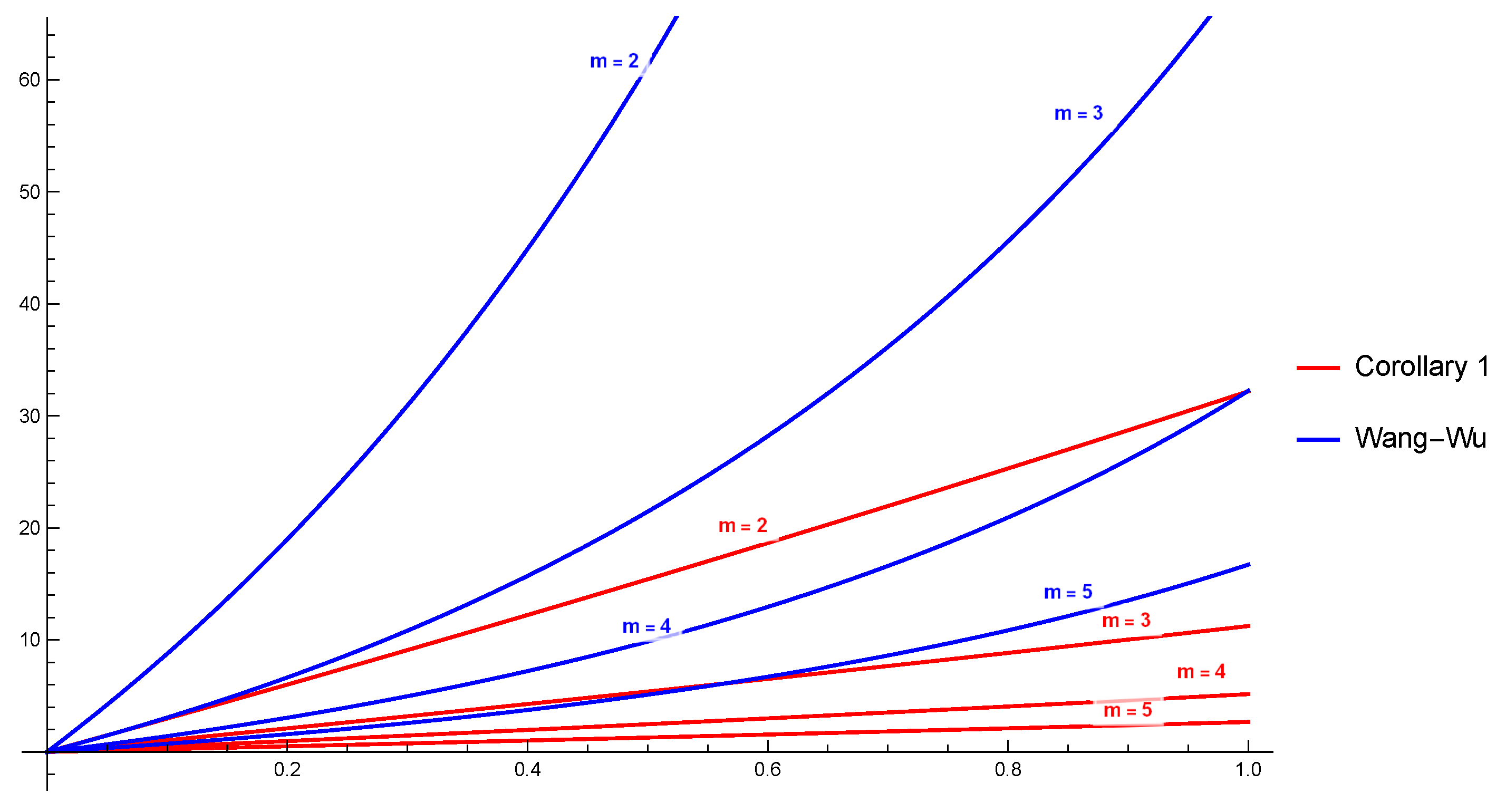
Let us show the improvement in error estimates in more explicit form. Figure 1 shows a graphical representation of the error estimate functions computed for $n=10$ and $m=2,\dots 5$. The red curve corresponds to the estimate from Corollary 1, given by $8n^3\lambda$. The blue curves represent the error estimate from Theorem 2

$${\displaystyle \frac{n^2(n-m)}{m(2m-1)(n-1)}}{h}_1\left(t\right).$$

This graphical comparison clearly demonstrates the improvement.

3.1. Some Special Cases of Wang–Zheng-Type Methods

This subsection is devoted to several particular cases obtained by choosing specific correction functions. We focus on three classical choices: Newton’s method, Halley’s method, and the Chebyshev-like method.

3.1.1. Wang-Zheng-Type with Newton’s Correction (WZN Method)

Let us consider the Wang-Zheng-type method (1) with Newton’s iteration function defined by $\Phi \left(x\right)=({\Phi }_1\left(x\right),\dots ,{\Phi }_s\left(x\right))$ with

$${\Phi }_i\left(x\right)=x_i-m_i{\displaystyle \frac{f\left(x_i\right)}{f^{\prime }\left(x_i\right)}}.$$

Kyncheva et al. [13] proved that Newton’s iteration function is an iteration function of the first kind at a point $\xi \in {\mathbb{C}}^s$ with control function $\omega$ of order $\mu =1$, defined by

$$\omega \left(t\right)={\displaystyle \frac{(n-m)t}{m-nt}}\mathrm{on}J=\left[0,{\displaystyle \frac{m}{n}}\right).$$

(53)

Corollary 2. 

Let $f\in \mathbb{C}\left[z\right]$ be a polynomial of degree $n\ge 2$ that splits in $\mathbb{C}$, let ${\xi }_1,\dots ,{\xi }_s$ be all distinct zeros of f with multiplicity $m_1,\dots ,m_s$ $(m_1+\dots +m_s=n)$, and let $\xi \in {\mathbb{C}}^s$ be a root vector of f. Suppose $x^{\left(0\right)}\in {\mathbb{C}}^s$ is an initial guess satisfying (45). Then, the Wang–Zheng-type method with Newton’s correction is well defined and converges to ξ with Q-order $r=5$ and with the following error estimates:

$$\parallel x^{(k+1)}-\xi \parallel ⪯{\left({\displaystyle \frac{1}{4n}}\right)}^{5^k}\parallel x^{\left(k\right)}-\xi \parallel ,$$

(54)

$$\parallel x^{\left(k\right)}-\xi \parallel ⪯{\left({\displaystyle \frac{1}{4n}}\right)}^{{\displaystyle \frac{5^k-1}{4}}}\parallel x^{\left(0\right)}-\xi \parallel ,$$

(55)

$$\parallel x^{(k+1)}{-\xi \parallel }_{\infty }\le 4n^3\delta {\left(\xi \right)}^{-4}{\parallel x^{\left(k\right)}-\xi \parallel }_{\infty }^5\mathit{for}\mathit{all}k\ge 0.$$

(56)

Proof. 

For Function $\omega$ defined by (53), we have

$${\displaystyle \frac{1}{2n}}\in J\mathrm{and}\omega \left({\displaystyle \frac{1}{2n}}\right)={\displaystyle \frac{n-m}{2mn-n}}<1,$$

(57)

therefore, (44) is satisfied. Based on Corollary 1, we determine that the Wang–Zheng-type method with Newton’s correction is well defined and converges to $\xi$ with Q-order $r=5$. It follows from (50), (49) and (53) that

$$\lambda ={\displaystyle \frac{{\lambda }_1}{{\lambda }_2}}\le {\displaystyle \frac{{(n-1)}^2(4n^2-3n+1)}{16n^5-44n^4+59n^3-43n^2-3}}<{\displaystyle \frac{1}{4n}},$$

where

$${\lambda }_1={(n-m)}^2(4(2m-1)n^2-4mn+m+n)$$

and

$$\begin{array}{ccc}\hfill {\lambda }_2& =& 2(2m-1)m(2n-1){((4m-2)n^2-2mn+m)}^2\hfill \\ & & -(n-1)(n-m)(4(2m-1)n^2+(1-4m)n+m).\hfill \end{array}$$

Also, we have ${\left(2n\right)}^{r-1}\lambda <4n^3$. Now, the estimates of Corollary 2 follow from those of Corollary 1. □

3.1.2. Wang–Zheng-Type with Halley’s Correction (WZH Method)

Let us consider the Wang–Zheng-type method (1) with Halley’s iteration function defined by $\Phi \left(x\right)=({\Phi }_1\left(x\right),\dots ,{\Phi }_s\left(x\right))$ with

$${\Phi }_i\left(x\right)=x_i-{\displaystyle \frac{f\left(x_i\right)}{f^{\prime }\left(x_i\right)}}{\left({\displaystyle \frac{m_i+1}{2m_i}}-{\displaystyle \frac{1}{2}}{\displaystyle \frac{f\left(x_i\right)}{f^{\prime }\left(x_i\right)}}{\displaystyle \frac{f^{″}\left(x_i\right)}{f^{\prime }\left(x_i\right)}}\right)}^{-1}.$$

Kyncheva et al. [13] proved that the Halley iteration function is an iteration function of the first kind at Point $\xi \in {\mathbb{C}}^s$ with Control Function $\omega$ of order $\mu =2$ defined by

$$\omega \left(t\right)={\displaystyle \frac{n(n-m)t^2}{2m(1-t)(m-nt)-n(n-m)t^2}}\mathrm{on}J=\left[0,{\displaystyle \frac{2m}{n+m+\sqrt{(n-m)(3n-m)}}}\right).$$

(58)

Corollary 3. 

Let $f\in \mathbb{C}\left[z\right]$ be a polynomial of degree $n\ge 2$ that splits in $\mathbb{C}$, let ${\xi }_1,\dots ,{\xi }_s$ be all distinct zeros of f with multiplicity $m_1,\dots ,m_s$ $(m_1+\dots +m_s=n)$, and let $\xi \in {\mathbb{C}}^s$ be a root vector of f. Suppose $x^{\left(0\right)}\in {\mathbb{C}}^s$ is an initial guess satisfying (45). Then, the Wang–Zheng-type method with Halley’s correction is well defined and converges to ξ with Q-order $r=6$ and with the following error estimates:

$$\parallel x^{(k+1)}-\xi \parallel ⪯{\left({\displaystyle \frac{1}{12n}}\right)}^{6^k}\parallel x^{\left(k\right)}-\xi \parallel ,$$

(59)

$$\parallel x^{\left(k\right)}-\xi \parallel ⪯{\left({\displaystyle \frac{1}{12n}}\right)}^{{\displaystyle \frac{6^k-1}{5}}}\parallel x^{\left(0\right)}-\xi \parallel ,$$

(60)

$$\parallel x^{(k+1)}{-\xi \parallel }_{\infty }\le {\displaystyle \frac{8}{3}}{n}^4\delta {\left(\xi \right)}^{-5}{\parallel x^{\left(k\right)}-\xi \parallel }_{\infty }^6\mathit{for}\mathit{all}k\ge 0.$$

(61)

Proof. 

For Function $\omega$ defined by (58), we have

$${\displaystyle \frac{1}{2n}}\in J\mathrm{and}\omega \left({\displaystyle \frac{1}{2n}}\right)={\displaystyle \frac{n-m}{8m^{2}n-4m^2-4mn+3m-n}}={\displaystyle \frac{n-m}{Z}}<1$$

therefore, (44) is satisfied. Based on Corollary 1, we obtain that the Wang–Zheng-type method with Halley’s correction is well defined and converges to $\xi$ with Q-order $r=6$. It follows from (50), (49) and (58) that

$$\lambda ={\displaystyle \frac{{\lambda }_3}{{\lambda }_4}}\le {\displaystyle \frac{{(n-1)}^2(12n^2-11n+3)}{144n^5-372n^4+419n^3-253n^2+81n-11}}<{\displaystyle \frac{1}{12n}},$$

where

$${\lambda }_3={(m-n)}^2(m+n(4Z-1)-2Z)$$

and

$$\begin{array}{ccc}\hfill {\lambda }_4& =& 2(2n-1)Z(m-n)(m^2(8n-4)-4mn+m+n)\hfill \\ & & +{(m-n)}^2(m^2(8n-4)-4mn+m+n)+2m(2m-1){(2n-1)}^3{Z}^2.\hfill \end{array}$$

Also, we have ${\left(2n\right)}^{r-1}\lambda <{\displaystyle \frac{8}{3}}{n}^4$. Now, the estimates of Corollary 3 follow from those of Corollary 1. □

3.1.3. Wang–Zheng-Type with Chebyshev-like Correction (WZCh Method)

Let us consider the Wang–Zheng-type method (1) with the Chebyshev-like iteration function defined by $\Phi \left(x\right)=({\Phi }_1\left(x\right),\dots ,{\Phi }_s\left(x\right))$ with

$${\Phi }_i\left(x\right)=x_i-m_i{\displaystyle \frac{f\left(x_i\right)}{f^{\prime }\left(x_i\right)}}\left(1+{\displaystyle \frac{f\left(x_i\right)}{f^{\prime }\left(x_i\right)}}\sum _{j\ne i}{\displaystyle \frac{m_j}{x_i-x_j}}\right).$$

Proinov and Cholakov [14] proved that the Chebyshev-like operator is an iteration function of the first kind at Point $\xi \in {\mathbb{C}}^s$ with Control Function $\omega$ of order $\mu =2$ defined by

$$\omega \left(t\right)={\displaystyle \frac{{(n-m)}^2(1-2t)+m(n-m)(1-t)}{(1-2t){(m-nt)}^2}}{t}^2\mathrm{on}J=\left[0,{\displaystyle \frac{m}{n}}\right).$$

(62)

Corollary 4. 

Let $f\in \mathbb{C}\left[z\right]$ be a polynomial of degree $n\ge 2$ that splits in $\mathbb{C}$, let ${\xi }_1,\dots ,{\xi }_s$ be all distinct zeros of f with multiplicity $m_1,\dots ,m_s$ $(m_1+\dots +m_s=n)$, and let $\xi \in {\mathbb{C}}^s$ be a root vector of f. Suppose $x^{\left(0\right)}\in {\mathbb{C}}^s$ is an initial guess satisfying (45). Then, the Wang–Zheng-type method with Chebyshev-like correction is well defined and converges to ξ with Q-order $r=6$ and with the following error estimates:

$$\parallel x^{(k+1)}-\xi \parallel ⪯{\left({\displaystyle \frac{1}{4n}}\right)}^{6^k}\parallel x^{\left(k\right)}-\xi \parallel ,$$

(63)

$$\parallel x^{\left(k\right)}-\xi \parallel ⪯{\left({\displaystyle \frac{1}{4n}}\right)}^{{\displaystyle \frac{6^k-1}{5}}}\parallel x^{\left(0\right)}-\xi \parallel ,$$

(64)

$$\parallel x^{(k+1)}{-\xi \parallel }_{\infty }\le 8n^4\delta {\left(\xi \right)}^{-4}{\parallel x^{\left(k\right)}-\xi \parallel }_{\infty }^5\mathit{for}\mathit{all}k\ge 0.$$

(65)

Proof. 

For Function $\omega$ defined by (62), we have

$${\displaystyle \frac{1}{2n}}\in J\mathrm{and}\omega \left({\displaystyle \frac{1}{2n}}\right)={\displaystyle \frac{(n-m)(m+2(n-1\left)n\right)}{2n^2(n-1){(2m-1)}^2}}<1$$

Therefore, condition (44) is satisfied. Therefore, it follows from Corollary 1 that the Wang–Zheng-type method with Chebyshev-like correction is well defined and converges to $\xi$ with Q-order $r=6$. It follows from (50), (49) and (62) that

$$\begin{array}{ccc}\hfill \lambda & \le & {\displaystyle \frac{(n-1)(2n^2-2n+1)(8n^3-6n^2+2n-1)}{64n^7-176n^6+236n^5-212n^4+132n^3-56n^2+17n-3}}<{\displaystyle \frac{1}{4n}}\hfill \end{array}$$

Also, we have ${\left(2n\right)}^{r-1}\lambda <8n^4$. Now, the estimates of Corollary 4 follow from those of Corollary 1. □

4. Kyurkchiev and Andreev Family

In 1990, Kyurkchiev and Andreev [15] constructed a family of iterative methods. For every given positive integer N, the N-method of this family has the order of convergence $3N+1$.

Definition 2 

(Kyurkchiev and Andreev [15]). Let $f\in \mathbb{C}\left[z\right]$ be a polynomial of degree $n\ge 2$. Define a sequence ${\left(T^{\left(N\right)}\right)}_{N=0}^{\infty }$ of iteration functions $T^{\left(N\right)}: D_N\subset {\mathbb{C}}^s\to {\mathbb{C}}^s$ as follows:

• ${\displaystyle T^{\left(0\right)}\left(x\right)=x}$;
• ${\displaystyle T^{\left(N\right)}}$ is the Wang–Zheng iteration function for multiple zeros with correction $T^{(N-1)}$ for $N\ge 1$.

Theorem 3 

(Kyurkchiev and Andreev [15]). Let $f\in \mathbb{C}\left[z\right]$ be a polynomial of degree $n\ge 2$ that splits in $\mathbb{C}$, let ${\xi }_1,\dots ,{\xi }_s$ be all distinct zeros of f with multiplicities $m_1,\dots ,m_s$, and let $N\ge 1$. Let $0<h<1$ and $c>0$ be such that

1. 

$\delta -4ch>0$;

2. 

${\displaystyle \frac{2chn}{{(\delta -4ch)}^2}\le \frac{1}{\delta -ch}}$;

3. 

$4chn<\delta -ch$;

4. 

${\displaystyle c^3{n}^2\left({\displaystyle 2+\frac{4ch}{\delta -ch}}\right)\frac{\delta -ch}{\delta -ch-2chn}\frac{1}{{(\delta -4ch)}^3}\le 1}$,

where $\delta ={\min }_{i\ne j}|{\xi }_i-{\xi }_j|$. Suppose $x^{\left(0\right)}\in {\mathbb{C}}^s$ is an initial approximation satisfying the following condition:

$$\parallel x^{\left(0\right)}{-\xi \parallel }_{\infty }\le ch,$$

(66)

where $\xi =({\xi }_1,\dots ,{\xi }_s)$. Then, the N-th Kyurkchiev–Andreev iterative method is well defined and converges to ξ with Q-order $r=3N+1$ and error estimate

$$\parallel x^{\left(k\right)}{-\xi \parallel }_{\infty }\le c{h}^{{(3N+1)}^k}\mathit{for}\mathit{all}k\ge 0.$$

(67)

Definition 3. 

We define a sequence ${\left({\varphi }_N\right)}_{N=0}^{\infty }$ of functions recursively by setting ${\varphi }_0\left(t\right)=1$ and

$${\varphi }_{N+1}\left(t\right)={\displaystyle \frac{n\left(n-m\right)A_N\left(t\right)B_N\left(t\right)}{2m(m-nt)-n(n-m)A_N\left(t\right)B_N\left(t\right)}},$$

(68)

where the functions $A_N$ and $B_N$ are defined by

$$A_N\left(t\right)={\displaystyle \frac{t^2{\varphi }_N\left(t\right)}{1-\overline{{\varphi }_N}\left(t\right)}},B_N\left(t\right)={\displaystyle \frac{t}{1-t}}+{\displaystyle \frac{t}{1-\overline{{\varphi }_N}\left(t\right)}},$$

(69)

$${\overline{\varphi }}_N\left(t\right)=t(1+{\varphi }_N\left(t\right)).$$

(70)

Let R be the smallest positive solution of ${\varphi }_1\left(t\right)=1$. It can easily be proven that for every integer $N\ge 1$:

• ${\varphi }_N$ is quasi-homogeneous of exact degree $\mu =3N$ on $[0,R]$ and ${\varphi }_N\left(R\right)=1$;
• ${\varphi }_N\left(t\right)\le \varphi {\left(t\right)}^N$ for every $t\in [0,R]$ (see Lemma 4.3 from [16]);
• ${\displaystyle T^{\left(N\right)}}$ is an iteration function of first kind at $\xi$ with control function $\omega : [0,R]\to {\mathbb{R}}_{+}$ defined by $\omega \left(t\right)={\varphi }_{N-1}\left(t\right)$ (this statement follows from Lemma 2).

Corollary 5. 

Let $f\in \mathbb{C}\left[z\right]$ be a polynomial of degree $n\ge 2$ that splits in $\mathbb{C}$, let ${\xi }_1,\dots ,{\xi }_s$ be all distinct zeros of f with multiplicity $m_1,\dots ,m_s$ $(m_1+\dots +m_s=n)$, let $\xi \in {\mathbb{C}}^s$ be a root vector of f, and let $N\ge 1$. Suppose that $x^{\left(0\right)}\in {\mathbb{C}}^s$ is an initial guess satisfying the following condition:

$$G\left(E\left(x^{\left(0\right)}\right)\right)>0,$$

(71)

where Function E is defined by (5) and Function G is defined by

$$G\left(t\right)=m(m-nt)-n\left(n-m\right)A\left(t\right)B\left(t\right)$$

(72)

and Functions A and B are defined by

$$A\left(t\right)={\displaystyle \frac{t^2}{1-2t}}\mathit{and}B\left(t\right)=t\left({\displaystyle \frac{1}{1-2t}}+{\displaystyle \frac{1}{1-t}}\right).$$

(73)

Then, the N-th Kyurkchiev–Andreev iterative method is well defined and converges to ξ with Q-order $r=3N+1$ and error estimates

$$\parallel x^{(k+1)}-\xi \parallel ⪯{\lambda }^{N{(3N+1)}^k}\parallel x^{\left(k\right)}-\xi \parallel ,\parallel x^{\left(k\right)}-\xi \parallel ⪯{\lambda }^{({(3N+1)}^k-1)/\left(3N\right)}\parallel x^{\left(0\right)}-\xi \parallel ,$$

(74)

for all $k\ge 0$ with $\lambda =\varphi \left(E\left(x^{\left(0\right)}\right)\right)$ defined by

$$\varphi \left(t\right)={\displaystyle \frac{n(n-m)A\left(t\right)B\left(t\right)}{2m(m-nt)-n(n-m)A\left(t\right)B\left(t\right)}}.$$

(75)

Proof. 

The statement follows from Theorem 1 for the Kyurkchiev–Andreev iterative method with control function $\omega : [0,R]\to {\mathbb{R}}_{+}$ defined by $\omega \left(t\right)={\varphi }_{N-1}\left(t\right)$ and the inequality ${\varphi }_N\left(t\right)\le \varphi {\left(t\right)}^N$. □

Let $0<h<1$ be a given number. Solving the equation $\varphi \left(t\right)=h^3$ in the interval $(0,R)$, we can reformulate Corollary 5 in the following equivalent form.

Corollary 6. 

Let $f\in \mathbb{C}\left[z\right]$ be a polynomial of degree $n\ge 2$ that splits in $\mathbb{C}$, let ${\xi }_1,\dots ,{\xi }_s$ be all distinct zeros of f with multiplicity $m_1,\dots ,m_s$ $(m_1+\dots +m_s=n)$, let $\xi \in {\mathbb{C}}^s$ be a root vector of f, and let $N\ge 1$. Suppose $x^{\left(0\right)}\in {\mathbb{C}}^s$ is an initial guess satisfying the following condition:

$$G_h\left(E\left(x^{\left(0\right)}\right)\right)>0,$$

(76)

where Function E is defined by (5), Function $G_h$ is defined by

$$G_h\left(t\right)=2h^{3}m(m-nt)-(1+h^3)n\left(n-m\right)A\left(t\right)B\left(t\right)$$

(77)

and Functions A and B are defined by (73). Then, the N-th Kyurkchiev–Andreev iterative method is well defined and converges to ξ with Q-order $r=3N+1$ and error estimate

$$\parallel x^{(k+1)}-\xi \parallel ⪯h^{3N{(3N+1)}^k}\parallel x^{\left(k\right)}-\xi \parallel ,\parallel x^{\left(k\right)}-\xi \parallel ⪯h^{{(3N+1)}^k-1}\parallel x^{\left(0\right)}-\xi \parallel$$

(78)

for all $k\ge 0$.

Proof. 

Let $R_h$ be the solution of $\varphi \left(t\right)=h^3$ in the interval $(0,R)$; then, $R_h<R$. From Corollary 5, we have that the N-th Kyurkchiev–Andreev iterative method is well defined and converges to $\xi$ with Error Estimate (74). Then, using $\lambda =\varphi \left(E\left(x^{\left(0\right)}\right)\right)\le \varphi \left(R_h\right)=h^3$, we obtain Error Estimate (78). □

Remark 2. 

We show that Corollary 6 is an improvement of the result of Kyurkchiev and Andreev (Theorem 3). If we summarize the first three conditions of Theorem 3, we have

$$0<c<{\displaystyle \frac{\delta }{h(1+4n)}}\mathrm{for}n\ge 3\mathit{and}0<c<{\displaystyle \frac{\delta }{10h}}\mathit{for}n=2.$$

The last condition is equivalent to

$${\displaystyle c^3{n}^2\left({\displaystyle 2+\frac{4ch}{\delta -ch}}\right)\frac{\delta -ch}{\delta -ch-2chn}\frac{1}{{(\delta -4ch)}^3}=\frac{2c^3(\delta +ch)n^2}{{(\delta -4ch)}^3(\delta -ch(2n+1))}\le 1.}$$

(79)

Therefore, c should be such that

$$0<c<\min \left\{{\displaystyle \frac{\delta }{h(1+4n)}},{\displaystyle \frac{\delta }{10h}},X_1\right\},$$

where $X_1$ is the solution of Inequality (79). Suppose that a vector $x^{\left(0\right)}\in {\mathbb{C}}^s$ satisfies (66). From ${\displaystyle 0<c<\frac{\delta }{h(1+4n)}}$, we have

$$E\left(x^{\left(0\right)}\right)={∥{\displaystyle \frac{x^{\left(0\right)}-\xi }{d\left(\xi \right)}}∥}_{\infty }\le {\displaystyle \frac{\parallel x^{\left(0\right)}{-\xi \parallel }_{\infty }}{\delta \left(\xi \right)}}\le {\displaystyle \frac{ch}{\delta \left(\xi \right)}}<{\displaystyle \frac{1}{1+4n}}.$$

Since $G_h$ is decreasing, we have

$$\begin{array}{ccc}& & G_h\left(E\left(x^{\left(0\right)}\right)\right)>G_h\left({\displaystyle \frac{1}{1+4n}}\right)={\displaystyle \frac{1}{2}}{h}^3(4m-1)\hfill \\ & +& {\displaystyle \frac{12h^{3}m-5h^3+12m-5}{64m(4n-1)}}+{\displaystyle \frac{4h^{3}m-h^3+4m-1}{32m{(4n-1)}^2}}+{\displaystyle \frac{20h^{3}m-3h^3-12m-3}{64m(4n+1)}}>0.\hfill \end{array}$$

Therefore, $x^{\left(0\right)}\in {\mathbb{C}}^s$ satisfies (76). Then, the N-th Kyurkchiev–Andreev iterative method is well defined and converges to ξ with Q-order $r=3N+1$ and Error Estimate (78). From the second estimate in (78) and (66), we get the estimate (67), which completes the proof.

5. Numerical Experiments

In this section, we present some numerical experiments. Let $f\in \mathbb{C}\left[z\right]$ be a polynomial of degree $n\ge 2$ with $s\ge 2$ distinct zeros $\xi =\{{\xi }_1,\dots ,{\xi }_s\}$ with multiplicity $m_{\xi }=\{m_1,\dots ,m_s\}$, respectively, $(m_1+\dots +m_s=n)$. In this paper, we study the local convergence of the Wang–Zheng-type methods for multiple zeros. We also derive the corresponding a priori and a posteriori error estimates. In the case of simple zeros, results of this kind can be reformulated as semilocal convergence theorems with computationally verifiable initial conditions and explicit error bounds (see [17]). However, in the more general case of multiple zeros, such transformation theorems are not available at present. For this reason, in the numerical examples below, we use a standard stopping criterion

$${\epsilon }_k=\underset{1\le i\le s}{\max }\left|f\left(x_i^{\left(k\right)}\right)\right|<{10}^{-15}.$$

(80)

The first polynomial is

$$f_1\left(z\right)=z^9-8z^8+25z^7-34z^6+64z^4-76z^3+8z^2+48z-32$$

with root-vector $\xi =\{-1,2,1+i,1-i\}$ with multiplicity $m_{\xi }=\{1,3,2,2\}$, respectively. In [18], Petković and Milošević choose the following initial guess

$$x^{\left(0\right)}=\{-1.1+0.2i,2.1-0.2i,0.8+1.2i,0.9-1.2i\}.$$

(81)

The second polynomial is

$$\begin{array}{ccc}\hfill f_2\left(z\right)& =& z^{15}-(8-3i)z^{14}+(28-24i)z^{13}-(58-86i)z^{12}+(81-190i)z^{11}-(86-287i)z^{10}\hfill \\ & & +(82-278i)z^9-(68-72i)z^8+(20+320i)z^7+(104-692i)z^6-(312-760i)z^5\hfill \\ & & +(464-384i)z^4-(320+256i)z^3-(128-576i)z^2+(384-384i)z-256\hfill \end{array}$$

with root-vector $\xi =\{-1,2,1+i,1-i,i,-2i\}$ with multiplicity $m_{\xi }=\{2,3,2,2,3,3\}$, respectively. The initial guess

$$x^{\left(0\right)}=\{-1.1+0.2i,2.2-0.1i,0.9+1.1i,0.8-1.1i,0.1+1.2i,0.2-1.9i\}$$

(82)

was taken from Milošević etc. [19]. Also, we consider the following polynomials with a second type initial guess; namely, Aberth’s initial approximation $x^{\left(0\right)}\in {\mathbb{C}}^s$ (see [20]) given by

$$x_{\nu }^{\left(0\right)}=-{\displaystyle \frac{a_1}{n{a}_0}}+r_0\exp \left(i{\theta }_{\nu }\right),{\theta }_{\nu }={\displaystyle \frac{\pi }{s}}\left(2\nu -{\displaystyle \frac{3}{2}}\right),\nu =1,\dots ,s.$$

(83)

Here, we use a rather rough choice for the radius $r_0=10$.

For each example and each of the considered methods, we present the smallest nonnegative integer k that satisfies the stopping criterion (80) for a prescribed accuracy $\epsilon <{10}^{-15}$.

Table 1. Numerical results for polynomial $f_1$.

Initial Guess	Method	Order	k	${\mathit{\epsilon }}_{\mathit{k}}$
Petković etc. (81)	W-Z with Newton	5	2	$1.09606424\times {10}^{-30}$
Petković etc. (81)	W-Z with Halley	6	2	$3.97454934\times {10}^{-47}$
Petković etc. (81)	W-Z with Chebyshev-like	6	2	$1.96609737\times {10}^{-19}$
Petković etc. (81)	K-A family ($N=1$)	4	2	$6.48816377\times {10}^{-18}$
Petković etc. (81)	K-A family ($N=10$)	31	1	$6.75082870\times {10}^{-39}$
Aberth’s ($r_0=10$) (83)	W-Z with Newton	5	10	$1.55176859\times {10}^{-11}$
Aberth’s ($r_0=10$) (83)	W-Z with Halley	6	11	$1.06114644\times {10}^{-11}$
Aberth’s ($r_0=10$) (83)	W-Z with Chebyshev-like	6	13	$8.19970743\times {10}^{-12}$
Aberth’s ($r_0=10$) (83)	K-A family ($N=1$)	4	11	$3.31841920\times {10}^{-11}$
Aberth’s ($r_0=10$) (83)	K-A family ($N=10$)	31	10	$6.69961607\times {10}^{-12}$

shows the obtained computational results for the polynomial $f_1$ using two types of initial guesses. For example, when the initial approximation proposed by Petkovi’c et al. (81) is used, the Wang–Zheng-type with Halley-like correction method computes all roots of the polynomial with a guaranteed accuracy of $3.97454934\times {10}^{-47}$ at the second iteration. The corresponding results for Polynomial $f_2$ are given in

Table 2. Numerical results for polynomial $f_2$.

Initial Guess	Method	Order	k	${\mathit{\epsilon }}_{\mathit{k}}$
Milošević etc. (82)	W-Z with Newton	5	2	$5.66824533\times {10}^{-24}$
Milošević etc. (82)	W-Z with Halley	6	2	$1.24036431\times {10}^{-38}$
Milošević etc. (82)	W-Z with Chebyshev-like	6	2	$4.01861869\times {10}^{-16}$
Milošević etc. (82)	K-A family ($N=1$)	4	2	$5.01208078\times {10}^{-15}$
Milošević etc. (82)	K-A family ($N=10$)	31	1	$2.02033778\times {10}^{-31}$
Aberth’s ($r_0=10$) (83)	W-Z with Newton	5	14	$1.06257588\times {10}^{-11}$
Aberth’s ($r_0=10$) (83)	W-Z with Halley	6	13	$2.96942022\times {10}^{-11}$
Aberth’s ($r_0=10$) (83)	W-Z with Chebyshev-like	6	13	$7.54981387\times {10}^{-11}$
Aberth’s ($r_0=10$) (83)	K-A family ($N=1$)	4	12	$1.14786427\times {10}^{-11}$
Aberth’s ($r_0=10$) (83)	K-A family ($N=10$)	31	10	$1.75140850\times {10}^{-11}$

.

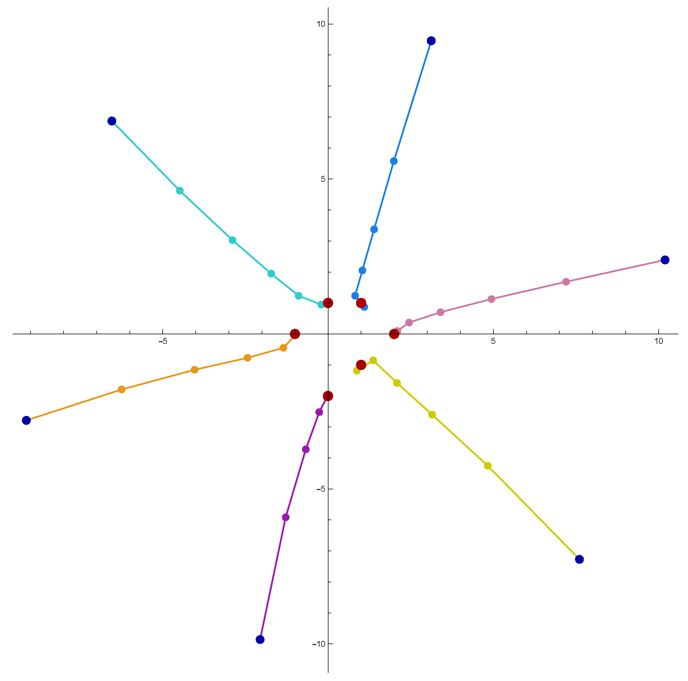
The trajectories of approximations for the Wang–Zheng-type with Chebyshev-like correction are presented in Figure 2. All initial guesses are presented with blue points, and roots of $f_2$ are preented with red points.

Remark 3. 

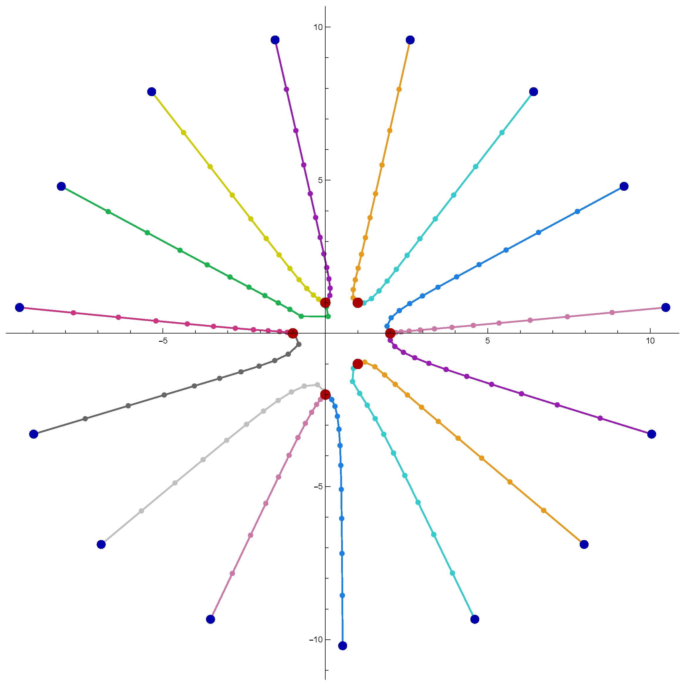
It is natural to consider the case when the multiplicities are unknown. In this situation, the methods can be applied by assuming unit multiplicities for all polynomial zeros, i.e., $m_{\xi }=\{1,1,\dots ,1\}$. Let us consider the Wang–Zheng-type (1) as a method with unknown multiplicities. We use the same test polynomials with Aberth’s initial approximation (83) with $r_0=10$. Again, we apply Stopping Criterion (80). The obtained results are very similar to those obtained in the case of known multiplicities. For example, for the Wang–Zheng-type method with Newton correction, the stopping criterion (80) is satisfied at the 21st iteration. The obtained accuracy is $3.670709830\times {10}^{-11}$. Figure 3 shows the trajectories of the approximations. Although the initial approximations are different, for each zero, the number of approximations that converge to it is equal to the multiplicity of that zero.

6. Conclusions

This paper presents a new family of simultaneous iterative methods with correction for the approximation of polynomial zeros with known multiplicities. The methods are constructed by combining the fourth-order Wang–Zheng iteration function with an arbitrary iteration function. A complete local convergence analysis is provided for a broad class of iteration functions. The obtained local convergence results improve earlier results from to Wang and Wu [12] and Kyurkchiev and Andreev [15] in several directions.

It is worth noting that a similar local convergence theorem can also be obtained in the case of simple zeros. Moreover, by applying the general convergence theory developed by Proinov [17], it is possible to derive a semilocal convergence theorem with computer-verifiable initial conditions. Such results are of practical importance. This direction provides a natural extension of the present work and will be considered in future studies.

References

1. Wang, X.-H.; Zheng, S.-M. A family of parallel and interval iterations for finding all roots of a polynomial simultaneously with rapid convergence. J. Comput. Math. 1984, 2, 70–76. [Google Scholar]
2. Nourein, A.W.M. An improvement on two iteration methods for simultaneous determination of the zeros of a polynomial. Intern. J. Comput. Math. 1977, 6, 241–252. [Google Scholar] [CrossRef] [Scilit]
3. Proinov, P.D.; Ivanov, S.I.; Petković, M.S. On the convergence of gander’s type family of iterative methods for simultaneous approximation of polynomial zeros. Appl. Math. Comput. 2019, 349, 168–183. [Google Scholar] [CrossRef] [Scilit]
4. Machado, R.N.; Lopes, L.G. Ehrlich-type methods with king’s correction for the simultaneous approximation of polynomial complex zeros. Math. Stat. 2019, 7, 129–134. [Google Scholar] [CrossRef] [Scilit]
5. Proinov, P.D.; Vasileva, M.T. A new family of high-order Ehrlich-type iterative methods. Mathematics 2021, 9, 1855. [Google Scholar] [CrossRef] [Scilit]
6. Proinov, P.; Ivanov, S. A new family of Sakurai-Torii-Sugiura type iterative methods with high order of convergence. J. Comput. Appl. Math. 2024, 436, 115428. [Google Scholar] [CrossRef] [Scilit]
7. Ivanov, S.I. Families of high-order simultaneous methods with several corrections. Numer. Algorithms 2024, 97, 945–958. [Google Scholar] [CrossRef] [Scilit]
8. Proinov, P. Unified convergence analysis for Picard iteration in n-dimensional vector spaces. Calcolo 2018, 55, 6–21. [Google Scholar] [CrossRef] [Scilit]
9. Proinov, P. Two classes of iteration functions and Q-convergence of two iterative methods for polynomial zeros. Symmetry 2021, 13, 371. [Google Scholar] [CrossRef] [Scilit]
10. Proinov, P.D.; Vasileva, M.T. On the convergence of high-order Gargantini-Farmer-Loizou type iterative methods for simultaneous approximation of polynomial zeros. Appl. Math. Comput. 2019, 361, 202–214. [Google Scholar] [CrossRef] [Scilit]
11. Proinov, P.D.; Vasileva, M.T. Local and semilocal convergence of Nourein’s iterative method for finding all zeros of a polynomial simultaneously. Symmetry 2020, 12, 1801. [Google Scholar] [CrossRef] [Scilit]
12. Wang, D.R.; Wu, Y.J. Some modifications of the parallel Halley iteration method and their convergence. Computing 1987, 38, 75–2022. [Google Scholar] [CrossRef] [Scilit]
13. Kyncheva, V.K.; Yotov, V.V.; Ivanov, S.I. Convergence of Newton, Halley and Chebyshev iterative methods as methods for simultaneous determination of multiple polynomial zeros. Appl. Numer. Math. 2017, 112, 146–154. [Google Scholar] [CrossRef] [Scilit]
14. Proinov, P.; Cholakov, S. Convergence of Chebyshev-like method for simultaneous approximation of multiple polynomial zeros. Proc. Bulg. Acad. Sci. 2014, 67, 907–918. [Google Scholar]
15. Kyurkchiev, N.; Andreev, A. On Halley-like algorithms with high order of convergence for simultaneous approximation of multiple roots of polynomials. Proc. Bulg. Acad. Sci. 1990, 43, 29–32. [Google Scholar]
16. Proinov, P.D.; Vasileva, M.T. On the convergence of high-order Ehrlich-type iterative methods for approximating all zeros of a polynomial simultaneously. J. Inequal. Appl. 2015, 336, 1–25. [Google Scholar] [CrossRef] [Scilit]
17. Proinov, P.D. Relationships between different types of initial conditions for simultaneous root finding methods. Appl. Math. Lett. 2016, 52, 102–111. [Google Scholar] [CrossRef] [Scilit]
18. Petković, M.; Milošević, D. Higher order methods for the inclusion of multiple zeros of polynomials. Reliab. Comput. 2011, 15, 91–108. [Google Scholar]
19. Milošević, D.M.; Petković, M.S.; Milošević, M.R. Improved methods for the simultaneous inclusion of multiple polynomial zeros. Appl. Math. Comput. 2014, 241, 332–346. [Google Scholar] [CrossRef] [Scilit]
20. Aberth, O. Iteration methods for finding all zeros of a polynomial simultaneously. Math. Comput. 1973, 27, 339–344. [Google Scholar] [CrossRef]
Figure 1. Graph of error estimates.
Axioms 15 00232 g001
Figure 2. Trajectories of approximations of polynomial roots for polynomial f 2 for Wang–Zheng-type method with Chebyshev-like correction.
Axioms 15 00232 g002
Figure 3. Trajectories of approximations of polynomial roots for polynomial f 2 for Wang–Zheng-type method with Newton correction with unknown multiplicities.
Axioms 15 00232 g003