ARIMA Model Selection and Prediction Intervals

Abstract

Inference after model selection is a very important problem. Model selection algorithms for ARIMA time series, with criteria such as AIC and BIC, tend to select an inconsistent model with positive probability, making data-splitting inference for testing and confidence intervals unreliable. One technique was fairly reliable for sample sizes greater than 600, and a modification also worked. Model selection is often useful for prediction, since the selected submodel tends to have fitted values and residuals that are highly correlated with those of the full model. A few prediction intervals perform fairly well even after model selection. A useful technique for handling outliers is to replace the outliers with missing values.

1. Introduction

This section reviews some time series models and model selection for ARIMA time series models. Section 2.1 shows that model selection algorithms for ARIMA time series, with criteria such as AIC and BIC, tend to select an inconsistent model with positive probability. There is one method that considers exactly one consistent model, and the probability that the consistent model is selected goes to one as the sample size $n\to \infty$. This procedure will be used to develop large sample $100(1-\delta )\%$ prediction intervals for $Y_{n+h}$ given a time series $Y_1,\dots ,Y_n$. In simulations, a commonly used prediction interval performs well even when inconsistent models are chosen. Some heuristics for this simulated performance will be given.

We will use the R software notation and write a moving average parameter $\theta$ with a positive sign. Many references and software programs write the model with a negative sign for the moving-average parameters. A moving-average MA($q)$ times series is

$$Y_t=\tau +{\theta }_1{e}_{t-1}+{\theta }_2{e}_{t-2}+\dots +{\theta }_q{e}_{t-q}+e_t$$

where ${\theta }_q\ne 0.$ An autoregressive AR($p)$ times series is

$$Y_t=\tau +{\varphi }_1{Y}_{t-1}+{\varphi }_2{Y}_{t-2}+\dots +{\varphi }_p{Y}_{t-p}+e_t$$

where ${\varphi }_p\ne 0.$ An autoregressive moving-average ARMA($p,q)$ times series is

$$Y_t=\tau +{\varphi }_1{Y}_{t-1}+{\varphi }_2{Y}_{t-2}+\dots +{\varphi }_p{Y}_{t-p}+{\theta }_1{e}_{t-1}+{\theta }_2{e}_{t-2}+\dots +{\theta }_q{e}_{t-q}+e_t$$

(1)

where ${\theta }_q\ne 0$ and ${\varphi }_p\ne 0.$ A time series $X_t$ follows an ARIMA($p,d,q$) model with known d if the differenced time series model $Y_t$ follows an ARMA($p,q$) model. See Box and Jenkins (1976) [1] for more on these models. We will assume that the $e_t$ are independent and identically distributed (iid) with zero mean and variance ${\sigma }^2$. The observed time series is $\left\{Y_t\right\}=Y_1,\dots ,Y_n$.

We usually want the ARMA($p,q)$ model to be weakly stationary, causal, and invertible. Let $Z_t=Y_t-\mu$ where $\mu =E\left(Y_t\right)$ if $\left\{Y_t\right\}$ is weakly stationary. Then, the causal property implies that $Z_t={\sum }_{j=1}^{\infty }{\psi }_j{e}_{t-j}+e_t$, which is an MA($\infty )$ representation, where the ${\psi }_j\to 0$ rapidly as $j\to \infty .$ Invertibility implies that $Z_t={\sum }_{j=1}^{\infty }{\chi }_j{Z}_{t-j}+e_t$, which is an AR($\infty )$ representation, where the ${\chi }_j\to 0$ rapidly as $j\to \infty .$ We will make the usual assumption that the AR(∞) and MA(∞) parameters are square summable. Thus, if the ARMA($p,q)$ model is weakly stationary, causal, and invertible, then $Y_t$ depends almost entirely on nearby lags of $Y_t$ and $e_t$, not on the distant past.

This paper considers model selection where it is known that the model is ARMA, AR, or MA, but the order needs to be determined. For ARMA model selection, let the full model F be an ARMA($p_{max},q_{max}$) model. For AR model selection $q_{max}=0$, while for MA model selection $p_{max}=0$. Granger and Newbold (1977, p. 178) [2] suggested using $p_{max}=13$ for AR model selection, and we may use $p_{max}=q_{max}=5$ for ARMA model selection, and $q_{max}=13$ for MA model selection. For ARMA model selection, there are $J=(p_{max}+1)(q_{max}+1)$ ARMA($p,q$) submodels where p ranges from 0 to $p_{max}$ and q ranges from 0 to $q_{max}$. For AR and MA model selection, there are $J=p_{max}+1$ and $J=q_{max}+1$ submodels, respectively. Assume the true (optimal) model is an ARMA($p_S,q_S$) model with $p_S\le p_{max}$ and $q_S\le q_{max}$. Let the selected model I be an ARMA($p_I,q_I$) model. Then, the model underfits unless $p_I\ge p_S$ and $q_I\ge q_S$.

More notation is needed for model selection. Let the full model be the AR($p_{max})$, MA($q_{max}$), or ARMA($p_{max},q_{max})$ model. Let $\mathit{\beta }$ be a $b\times 1$ vector. For the ARMA model selection, let $\mathit{\beta }={({\mathit{\varphi }}^T,{\mathit{\theta }}^T)}^T={({\varphi }_1,\dots ,{\varphi }_{p_{max}},{\theta }_1,\dots ,{\theta }_{q_{max}})}^T$ with $b=p_{max}+q_{max}$. For AR model selection, let $\mathit{\beta }={({\varphi }_1,\dots ,{\varphi }_{p_{max}})}^T$ with $b=p_{max}$, and for MA model selection, let $\mathit{\beta }={({\theta }_1,\dots ,{\theta }_{q_{max}})}^T$ with $b=q_{max}$. Hence, $\mathit{\beta }={({\beta }_1,\dots ,{\beta }_{p_{max}},{\beta }_{p_{max}+1},\dots ,{\beta }_{p_{max}+q_{max}})}^T$. Let $S=\{1,\dots ,p_S,p_{max}+1,\dots ,p_{max}+q_S\}$ index the true ARMA($p_S,q_S$) model. If $S=\varnothing$ is the empty set, then the time series random variables $Y_1,\dots ,Y_n$ are iid. Let $I=\{1,\dots ,p_I,p_{max}+1,\dots ,p_{max}+q_I\}$ index the ARMA($p_I,q_I)$ model. Let ${\widehat{\mathit{\beta }}}_{I,0}$ be a $b\times 1$ estimator of $\mathit{\beta }$ which is a obtained by padding ${\widehat{\mathit{\beta }}}_I$ with zeroes. If ${\mathit{\beta }}_I={({\varphi }_1,\dots ,{\varphi }_{p_I},{\theta }_1,\dots ,{\theta }_{q_I})}^T$, then ${\widehat{\mathit{\beta }}}_{I,0}={({\widehat{\varphi }}_1,\dots ,{\widehat{\varphi }}_{p_I},0,\dots ,0,{\widehat{\theta }}_1,\dots ,{\widehat{\theta }}_{q_I},0,\dots ,0)}^T.$ If $q_I=0$, then ${\widehat{\mathit{\beta }}}_{I,0}={({\widehat{\varphi }}_1,\dots ,{\widehat{\varphi }}_{p_I},0,\dots ,0)}^T.$ If $p_I=0$ then ${\widehat{\mathit{\beta }}}_{I,0}={(0,\dots ,0,{\widehat{\theta }}_1,\dots ,{\widehat{\theta }}_{q_I},0,\dots ,0)}^T.$ If $I=\varnothing$ with $p_I=q_I=0$, then define ${\widehat{\mathit{\beta }}}_{I,0}=0$, the $b\times 1$ vector of zeroes. The submodel I underfits unless $S\subseteq I$.

For example, if $p_{max}=q_{max}=5$, then $S=\{1,6,7\}$ corresponds to the ARMA(1,2) model, and $I=\{1,6,7,8\}$ corresponds to the ARMA(1,3) model. Then, ${\widehat{\mathit{\beta }}}_S={({\widehat{\varphi }}_1,{\widehat{\theta }}_1,{\widehat{\theta }}_2)}^T$, ${\widehat{\mathit{\beta }}}_{S,0}={({\widehat{\varphi }}_1,0,0,0,0,{\widehat{\theta }}_1,{\widehat{\theta }}_2,0,0,0)}^T$, and ${\widehat{\mathit{\beta }}}_{I,0}={({\widehat{\varphi }}_1,0,0,0,0,{\widehat{\theta }}_1,{\widehat{\theta }}_2,{\widehat{\theta }}_3,0,0)}^T$.

The model $I_{min}$ corresponds to the model that minimizes the AIC, $AI{C}_C$, or BIC criterion. Then the model selection estimator ${\widehat{\mathit{\beta }}}_{MS}={\widehat{\mathit{\beta }}}_{I_{min},0}$. Haile and Olive (2024) [3] gave some large-sample theory for ${\widehat{\mathit{\beta }}}_{MS}$.

For AR model selection, the probability of underfitting goes to 0 if the Akaike (1973) [4] AIC, Schwartz (1978) [5] BIC, or Hurvich and Tsai (1989) [6] $AI{C}_C$ criterion are used. See Hannan and Quinn (1979) [7] and Shibata (1976) [8]. Although Hannan (1980)  [9], Hannan and Kavalieris (1984) [10], and Huang et al. (2022) [11] gave similar results for ARMA models, in simulations, BIC did not appear to select a consistent model, with probability approaching one. AIC and $AI{C}_C$ appear to fail due to the following Theorem 1 for the Gaussian maximum likelihood estimator (GMLE).

Let the $r_i$ be the m (one step ahead) residuals, where often $m=n$ or $m=n-p$. Under regularity conditions,

$${\tilde{\sigma }}^2={\displaystyle \frac{{\sum }_{i=1}^m{r}_i^2}{m-p-q-c}}$$

(2)

is a consistent estimator of ${\sigma }^2$, where often $c=0$ or $c=1$. See Davis (1977) [12] and Granger and Newbold (1977, p. 85) [2]. Huang et al. (2022) [11] argued that estimators of ${\sigma }^2$ could be good even when the time series models overfit. Let ${\widehat{\sigma }}^2$ be the estimator of ${\sigma }^2$ produced by the time series model, and let ${\gamma }_k=Cov(Y_t,Y_{t-k})$. Let

$${\mathbf{\Gamma }}_n=\left[\begin{array}{cccc}{\gamma }_0& {\gamma }_1& \dots & {\gamma }_{n-1}\\ {\gamma }_1& {\gamma }_0& \dots & {\gamma }_{n-2}\\ ⋮& ⋮& \ddots & ⋮\\ {\gamma }_{n-1}& {\gamma }_{n-2}& \dots & {\gamma }_0\end{array}\right].$$

The following large sample theorem for the AR(p) model is due to Mann and Wald (1943) [13]. Also see McElroy and Politis (2020, p. 333) [14] and Anderson (1971, pp. 210–217) [15]. For large sample theory for MA and ARMA models, see Hannan (1973) [16], Kreiss (1985) [17], and Yao and Brockwell (2006) [18].

There is a strong regularity condition for the GMLE for the ARMA model. Assume the ARMA($p_S,q_S$) model is the true model. If both $p>p_S$ and $q>q_S$, then the GMLE is not a consistent estimator. See Chan, Ling, and Yau (2020) [19] and Hannan (1980) [9].  

Theorem 1. 

Let the iid zero mean $e_i$ have variance ${\sigma }^2$, and let the time series have mean $E\left(Y_t\right)=\mu$.

(a) Let $Y_1,\dots ,Y_n$ be a weakly stationary and invertible AR(p) time series, and let $\mathit{\beta }={({\varphi }_1,\dots ,{\varphi }_p)}^T$. Let $\widehat{\mathit{\beta }}$ be the Yule Walker estimator of $\mathit{\beta }$. Then,

$$\sqrt{n}(\widehat{\mathit{\beta }}-\mathit{\beta })\stackrel{D}{\to }{N}_p(\mathbf{0},\mathit{V})$$

(3)

where $\mathit{V}=\mathit{V}\left(\mathit{\beta }\right)={\sigma }^2{\mathbf{\Gamma }}_p^{-1}.$ Equation (3) also holds under mild regularity conditions for the least squares estimator, and the GMLE of $\mathit{\beta }$.

(b) Let $Y_1,\dots ,Y_n$ be a weakly stationary, causal, and invertible MA(q) time series, and let $\mathit{\beta }={({\theta }_1,\dots ,{\theta }_q)}^T$. Let $\widehat{\mathit{\beta }}$ be the GMLE. Under regularity conditions,

$$\sqrt{n}(\widehat{\mathit{\beta }}-\mathit{\beta })\stackrel{D}{\to }{N}_q(0,\mathit{V})$$

(4)

where V is given, for example, by McElroy and Politis (2022, pp. 340–341) [14].

(c) Let $Y_1,\dots ,Y_n$ be a weakly stationary, causal, and invertible ARMA($p,q$) time series, and let $\mathit{\beta }={({\varphi }_1,\dots ,{\varphi }_p,{\theta }_1,\dots ,{\theta }_q)}^T$ with $g=p+q$. Let $\widehat{\mathit{\beta }}$ be the GMLE. Under regularity conditions,

$$\sqrt{n}(\widehat{\mathit{\beta }}-\mathit{\beta })\stackrel{D}{\to }{N}_g(0,\mathit{V}),$$

(5)

where V depends on the autocorrelation function and ${\sigma }^2$.

The main point of Theorem 1 is that the theory can hold even if the $e_t$ are not iid $N(0,{\sigma }^2).$ The basic idea for the GMLE is that $\left\{Y_t\right\}$ satisfies an AR(∞) model which is approximately an AR($p_y$) model, and the large sample theory for the AR($p_y$) model depends on the zero mean error distribution through ${\sigma }^2$ by Theorem 1(a). See Anderson (1971: ch. 5) [15], Anderson (1977) [20], Durbin (1959) [21], Hamilton (1994, pp. 117, 429) [22], and Hannan and Rissanen (1982, p. 85) [23]. When the $e_t$ are iid $N(0,{\sigma }^2)$, $\mathit{V}=\mathit{V}\left(\mathit{\beta }\right)={\mathit{I}}_1^{-1}\left(\mathit{\beta }\right)$, the inverse information matrix. Then, for the AR(p) model, $\mathit{V}\left(\mathit{\varphi }\right)={\sigma }^2{\mathbf{\Gamma }}_p^{-1}\left(\mathit{\varphi }\right)={\mathit{I}}_1^{-1}\left(\mathit{\varphi }\right)$. See Box and Jenkins (1976, p. 241) [1] and McElroy and Politis (2020, pp. 340–344) [14].

Pötscher (1994) [24] showed how to estimate $r_S=max(p_S,q_S)$ consistently. Section 2.1 reviews this method and proposes a modification that can lead to a more parsimonious model. Section 2.2 illustrates h-step ahead prediction intervals with ARIMA models. Section 2.3 gives some examples and simulations.

2. Materials and Methods

2.1. Model Selection Algorithms

In the literature and software, the AIC and BIC criteria can take many forms since the criterion can be multiplied by a positive constant, such as $1/n$, and a constant $d_n$ can be added to the criterion without changing the model that minimizes the criterion. Parameters that are in every model, such as ${\sigma }^2$ and possibly a constant, can be absorbed in a constant $d_n$. For ARMA($p,q$) models, let $log\left(\widehat{L}\right)$ be the log likelihood for the GMLE. Then the AIC and BIC criteria have the form $-2log\left(\widehat{L}\right)+(p+q)c\left(n\right)$ where $c\left(n\right)=2$ for AIC and $c\left(n\right)=log\left(n\right)$ for BIC. From McElroy and Politis (2020, p. 360) [14] and Huang et al. (2022) [11], $-2log\left(\widehat{L}\right)\approx nlog\left({\widehat{\sigma }}_I^2\right)+a_n$, where ${\widehat{\sigma }}_I^2$ is the GMLE of the error variance of model I and $a_n$ is a constant that depends on n. Hence, if I is an ARMA($p,q$) model, take

$$AIC\left(I\right)=nlog\left({\widehat{\sigma }}_I^2\right)+2(p+q)andBIC\left(I\right)=nlog\left({\widehat{\sigma }}_I^2\right)+(p+q)log\left(n\right).$$

(6)

For AIC given by (6), let $\Delta \left(I\right)=AIC\left(I\right)-AIC\left(I_{min}\right)$, then models with $\Delta \left(I\right)\le 2$ are “good,” and models with $4\le \Delta \left(I\right)\le 7$ are borderline. See Duong (1984) [25]. Claeskens and Hjort (2008, pp. 39, 111) [26] use slightly different formulas for AR(p) models. Pötscher and Srinivasan (1994) [27] multiply the Equation (6) formulas by $1/n$.

In simulations for ARMA model selection, the model selection methods often failed to select a consistent model with high probability in that an inconsistent model was selected with probability $>0.1$. A model I is inconsistent due to underfitting if $p_I<p_S$ or $q_I<q_S$. A model I is inconsistent due to overfitting if $p_I>p_S$ and $q_I>q_S$. A model I is consistent if $p_I=p_S$ and $q_I\ge q_S$ or if $q_I=q_S$ and $p_I\ge p_S$. If the model selection procedure were restricted to AR or MA models, then model I would be inconsistent only due to underfitting. The BIC criterion appeared to work for large n if the only models considered were the ARMA($k,k$) models for $k=0,\dots ,k_{max}$. Then the only consistent model is the ARMA($r_S,r_S)$ model, assuming $r_S=max(p_S,q_S)\le k_{max}$. For this set of restricted models, $AIC$ and $AI{C}_C$ tend to overfit with positive probability if $r_S<k_{max}$, and hence do not select a consistent model with probability going to one as $n\to \infty$.

In simulations, the Pötscher (1990) [24] method to estimate $r_S=max(p_S,q_S)$ often worked rather well. Also see Pötscher and Srinivasan (1994) [27]. Chan, Ling, and Yau (2020) [19] suggested that this method is reliable for $n\ge 1000.$ In our simulations, the method was fairly reliable for $n\ge 600$, but some models needed much larger n, and there were some models where the method did not simulate well. For the Pötscher (1990) [24] method, let $k_{max}$ be a positive integer such as $p_{max}=q_{max}=k_{max}=5$. Fit the ARMA($k,k$) model for $k=0,1,\dots ,k_{max}$. For each of these $k_{max}+1$ models, compute the BIC–type criterion $z\left(k\right)=log\left({\widehat{\sigma }}_k^2\right)+2klog\left(n\right)/n$ where ${\widehat{\sigma }}_k^2$ is the GMLE estimator of the error (or innovation) variance ${\sigma }^2$. This criterion is Equation (6) divided by n, and thus (6) could be used instead. The estimator $\widehat{r}$ of $r_S$ is the first local minimum of the series $z\left(0\right),z\left(1\right),\dots ,z\left(k_{max}\right)$. Hence $\widehat{r}=0$ if $z\left(0\right)\le z\left(1\right)$; $\widehat{r}=1$ if $z\left(0\right)>z\left(1\right)$ and $z\left(1\right)\le z\left(2\right)$; $\widehat{r}=2$ if $z\left(0\right)>z\left(1\right)$, $z\left(1\right)>z\left(2\right)$, and $z\left(2\right)\le z\left(3\right)$; $\widehat{r}=k$ if $z\left(r\right)>z(r+1)$ for $0\le r<k$ and $z\left(k\right)\le z(k+1)$ for $k=0,\dots ,k_{max}-1$; and $\widehat{r}=k_{max}$ if $z\left(k\right)$ is not a local minimum for any $k=0,1,\dots ,k_{max}-1$. Note that $r_S\le k_{max}$ is necessary for $\widehat{r}$ to be a consistent estimator of $r_S$.

The following method is new and can have fewer parameters than the ARMA($\widehat{r},\widehat{r}$) model. Use the AIC(I) criterion of Equation (6) after finding $\widehat{r}$ as above. Then, a decrease in AIC $>2$ when one parameter is omitted suggests that the parameter was not needed. Let $pen$ be a penalty such as $pen=2$ (used in the simulations) or $pen=0$. The algorithm computes the $crit=AIC\left(I\right)-pen$ for the ARMA($\widehat{r},\widehat{r}$) model, and fits the ARMA($\widehat{r}-i,\widehat{r}$) and ARMA($\widehat{r},\widehat{r}-i)$ models for $i=0,\dots ,\widehat{r}-1$. If one of the models has AIC(I) $<crit$, then the set crit = AIC(I) $-pen$. This process is repeated at each step. The value of $crit$ is updated only if a decrease of more than $pen$ from the current value of $crit$ is observed. The final model I is the model selected by this algorithm. This additional penalty reduced underfitting. Note that $2\widehat{r}$ models are fitted after finding $\widehat{r}$, which fits $k_{max}+1$ models. This method is faster than computing the AIC for ${(k_{max}+1)}^2$ models. Take the ARMA($p,\widehat{r}$) or ARMA($\widehat{r},q$) model that has the smallest value of $crit$. Then at least one of p and q will equal $\widehat{r}$. Huang et al. (2022) [11] use a similar method with BIC.

Remark 1. 

Let the full model F be an ARMA($p_{max},q_{max}$) model. Assume that the full model does not overfit too severely, e.g., use $p_{max}=q_{max}=5$. Let r and $\widehat{Y}$ denote the residuals and fitted values from the full model. Let $r_I$ and ${\widehat{Y}}_I$ denote the residuals and fitted values from the submodel I. Let $cor$ denote the sample correlation. Empirically, good ARMA time series model selection estimators select a submodel I such that both $cor(r,r_I)$ and $cor(\widehat{Y},{\widehat{Y}}_I)$ are very high, and the plotted points, in both an RR plot of $r_I$ versus r and an FF plot of ${\widehat{Y}}_I$ versus $\widehat{Y}$, should cluster tightly about the identity line with zero intercept and unit slope. Then model I is often “good” for prediction, even if I underfits or overfits.

Note that $nlog\left({\widehat{\sigma }}_I^2\right)=nlog({\widehat{\sigma }}_I^2/{\widehat{\sigma }}_F^2)+nlog\left({\widehat{\sigma }}_F^2\right)$ where the last term acts as a constant. For large n, the term $nlog({\widehat{\sigma }}_I^2/{\widehat{\sigma }}_F^2)$ cannot get much below 0, and the term tends to be near zero if $cor(r,r_I)$ is very high so that the full model residuals and submodel residuals are nearly identical.

A lower bound on $cor(r,r_I)$ can be found for one model selection estimator. Fit the full ARMA($p_{max},q_{max}$) model with the GMLE. Let $r_i={\widehat{e}}_i$. Let the full multiple linear regression working model be

$$Y_t=\tau +{\varphi }_1{Y}_{t-1}+{\varphi }_2{Y}_{t-2}+\dots +{\varphi }_{p_{max}}{Y}_{t-p_{max}}+{\theta }_1{\widehat{e}}_{t-1}+{\theta }_2{\widehat{e}}_{t-2}+\dots +{\theta }_{q_{max}}{\widehat{e}}_{t-q_{max}}+e_t$$

(7)

for $t=max(p_{max},q_{max})+1,\dots ,n$. Let $m=n-max(p_{max},q_{max}).$ Do model selection for multiple linear regression using ordinary least squares and the Mallows (1973) [28] $C_p\left(I\right)$ criterion. Let r be the full model residuals from the full model (7). Let $r_I$ be the residuals from the ordinary least squares fit to submodel I. Let $d=p_{max}+q_{max}+1$ be the number of regression parameters for model (7). For the full model, $C_p\left(F\right)=d$. This method can also be used for AR(∞) models.

Theorem 2. 

Using the above notation, let model I use k parameters, including a constant. Assume the design matrix for the full working model (7) has full rank d. If $C_P\left(I\right)\le 2k$, then

$$cor(r,r_I)\ge \sqrt{1-{\displaystyle \frac{d}{m}}}.$$

Proof. 

Olive and Hawkins (2005) [29] proved that if the design matrix has full rank p with n cases with $C_P\left(I\right)\le 2k$, then

$$cor(r,r_I)=\sqrt{{\displaystyle \frac{n-p}{C_p\left(I\right)+n-2k}}}\ge \sqrt{1-{\displaystyle \frac{p}{n}}}.$$

Plug in d for p and m for n to get the result.    □

Remark 2. 

Note that $m\ge 20d$ implies that $cor(r,r_I)\ge \sqrt{19/20}=0.9747.$ If $\Delta \left(I\right)=AIC\left(I\right)-AIC\left(I_{min}\right)\le 2,$ then typically $cor(r,r_I)$, $cor(\widehat{Y},{\widehat{Y}}_I)$, $cor(r_S,r_I)$, and $cor({\widehat{Y}}_S,{\widehat{Y}}_I)$, will be high if $m\ge 20d$. If model averaging or Bayesian methods give nearly all the weight to models I, whose residuals and fitted values are highly correlated with those of the full model, then these methods may be useful for prediction. Model averaging is sometimes used for AR(∞) models. See, for example, references in Bürkner, Gabry, and Vehtari (2020) [30] and Liao et al. (2021) [31].

2.2. Prediction Intervals

For forecasting, predict the test data $Y_{n+1},\dots ,Y_{n+L}$ given the past training data $Y_1,\dots ,Y_n$. A large sample $100(1-\delta )\%$ prediction interval (PI) for $Y_{n+h}$ is $[L_n,U_n]$ where the coverage $P(L_n\le Y_{n+h}\le U_n)=1-{\delta }_n$ is eventually bounded below by $1-\delta$ as $n\to \infty$. We often want $1-{\delta }_n\to 1-\delta$ as $n\to \infty$. By construction, some of the prediction intervals will have training data coverage $\approx 1-{\delta }_n$ where $1-{\delta }_n\ge 1-\delta$, and $1-{\delta }_n\to 1-\delta$ as $n\to \infty$. A large sample $100(1-\delta )\%$ PI is asymptotically optimal if it has the shortest asymptotic length: the length of $[L_n,U_n]$ converges to $U_s-L_s$ as $n\to \infty$ where $[L_s,U_s]$ is the population shorth: the shortest interval covering at least $100(1-\delta )\%$ of the mass.

The shorth estimator of the population shorth will be defined below and used to create large sample PIs that do not require knowing the distribution of the errors $e_t$. If the data are $Z_1,\dots ,Z_n$, let $Z_{\left(1\right)}\le \dots \le Z_{\left(n\right)}$ be the order statistics. Let $\lceil x\rceil$ denote the smallest integer greater than or equal to x (e.g., $\lceil 7.7\rceil =8$). Consider intervals that contain c cases $[Z_{\left(1\right)},Z_{\left(c\right)}],[Z_{\left(2\right)},Z_{(c+1)}],\dots ,[Z_{(n-c+1)},Z_{\left(n\right)}]$. Compute $Z_{\left(c\right)}-Z_{\left(1\right)},Z_{(c+1)}-Z_{\left(2\right)},\dots ,Z_{\left(n\right)}-Z_{(n-c+1)}$. Then the estimator shorth(c) $=[Z_{\left(s\right)},Z_{(s+c-1)}]$ is the interval with the shortest length.

Suppose the data $Z_1,\dots ,Z_n$ are iid and a large sample $100(1-\delta )\%$ PI is desired for a future value $Z_f$ such that $P(Z_f\in [L_n,U_n])\to 1-\delta$ as $n\to \infty$. The shorth(c) interval is a large sample $100(1-\delta )\%$ PI if $c/n\to 1-\delta$ as $n\to \infty$, that often has the asymptotically shortest length. Frey (2013) [32] showed that for large $n\delta$ and iid data, the shorth(${\displaystyle k_n=\lceil n(1-\delta )\rceil }$) prediction interval has maximum undercoverage $\approx 1.12\sqrt{\delta /n}$, and used the large sample $100(1-\delta )\%$ PI shorth(c) =

$$[Z_{\left(s\right)},Z_{(s+c-1)}]withc=min(n,\lceil n[1-\delta +1.12\sqrt{\delta /n}]\rceil ).$$

(8)

Some more notation is needed before deriving PIs for time series. Suppose the training data set is $Y_1,\dots ,Y_t$. The h-step ahead forecast for a future value $Y_{t+h}$ is ${\widehat{Y}}_t\left(h\right)$ and the h-step ahead forecast residual is ${\widehat{e}}_t\left(h\right)=Y_{t+h}-{\widehat{Y}}_t\left(h\right).$ For example, a common choice for model $Y_t=\tau +{\sum }_i{\psi }_i{Y}_{t-i{k}_i}+{\sum }_j{\nu }_j{e}_{t-j{k}_j}+e_t$ is ${\widehat{Y}}_t\left(h\right)=\widehat{\tau }+{\sum }_i{\widehat{\psi }}_i{Y}_{t+h-i{k}_i}^{\ast }+{\sum }_j{\widehat{\nu }}_j{\widehat{e}}_{t+h-j{k}_j}^{\ast }$ where ${\widehat{e}}_t$ is the tth residual, $Y_{t+h-i{k}_i}^{\ast }=Y_{t+h-i{k}_i}$ if $h-i{k}_i\le 0,$ $Y_{t+h-i{k}_i}^{\ast }={\widehat{Y}}_t(h-i{k}_i)$ if $h-i{k}_i>0$, ${\widehat{e}}_{t+h-j{k}_j}^{\ast }={\widehat{e}}_{t+h-j{k}_j}$ if $h-j{k}_j\le 0,$ and ${\widehat{e}}_{t+h-j{k}_j}^{\ast }=0$ if $h-j{k}_j>0$, and the forecasts ${\widehat{Y}}_t\left(1\right),{\widehat{Y}}_t\left(2\right),\dots ,{\widehat{Y}}_t\left(L\right)$ are found recursively if there is data $Y_1,\dots ,Y_t$. Typically, the residuals ${\widehat{e}}_t={\widehat{e}}_{t-1}\left(1\right)$ are the 1-step ahead forecast residuals, and the fitted or predicted values ${\widehat{Y}}_t={\widehat{Y}}_{t-1}\left(1\right)$ are the 1-step ahead forecasts.

The following example is useful to illustrate the forecasts. The R software 4.5.3 produces ${\widehat{e}}_t$ and ${\widehat{Y}}_t=Y_t-{\widehat{e}}_t$ for $t=m+1,\dots ,m+n_1$ where there are $n_1$ 1-step ahead forecast residuals ${\widehat{e}}_t={\widehat{e}}_{t-1}\left(1\right)$ available, often with $m=0$ and $n_1=n$. In the examples, we obtain the formulas ${\widehat{Y}}_n\left(h\right)$ and then replace n by t so that the test-data formula is applied to the training data. Then, the general formula for an ARMA($p,q$) model is ${\widehat{Y}}_t\left(h\right)=\widehat{\tau }+{\widehat{\varphi }}_1{\widehat{Y}}_t(h-1)+{\widehat{\varphi }}_2{\widehat{Y}}_t(h-2)+\dots +{\widehat{\varphi }}_{h-1}{\widehat{Y}}_t\left(1\right)+{\widehat{\varphi }}_h{Y}_t+\dots +{\widehat{\varphi }}_p{Y}_{t+h-p}+{\widehat{\theta }}_h{\widehat{e}}_t+\dots +{\widehat{\theta }}_q{\widehat{e}}_{t+h-q}$ for $1<h\le min(p,q)$. Assume there are $n_h$ forecast residuals ${\widehat{e}}_t\left(h\right)$ available from the training data.

Example 1. 

Suppose the training data is $Y_1,\dots ,Y_n$. (a) Consider an MA(2) model: $Y_t=\tau +{\theta }_1{e}_{t-1}+{\theta }_2{e}_{t-2}+e_t$. The R software produces ${\widehat{e}}_t=Y_t-{\widehat{Y}}_t$. Thus, ${\widehat{Y}}_t=Y_t-{\widehat{e}}_t$ and $Y_t={\widehat{Y}}_t+{\widehat{e}}_t$. Then, ${\widehat{Y}}_t={\widehat{Y}}_{t-1}\left(1\right)=\widehat{\tau }+{\widehat{\theta }}_1{\widehat{e}}_{t-1}+{\widehat{\theta }}_2{\widehat{e}}_{t-2}$ for $t=1,\dots ,n$, and ${\widehat{e}}_t\left(1\right)=Y_{t+1}-{\widehat{Y}}_t\left(1\right)$ for $t=3,\dots ,n$. Also, ${\widehat{Y}}_n\left(1\right)=\widehat{\tau }+{\widehat{\theta }}_1{\widehat{e}}_n+{\widehat{\theta }}_2{\widehat{e}}_{n-1}$. Hence, there are $n_1=n$ 1-step ahead forecast residuals ${\widehat{e}}_t={\widehat{e}}_{t-1}\left(1\right)$ available. Similarly, ${\widehat{Y}}_t\left(2\right)=\widehat{\tau }+{\widehat{\theta }}_2{\widehat{e}}_t$ for $t=1,\dots ,n$. Hence, the 2-step ahead forecast residuals are available for $t=3,\dots ,n-2$. Now ${\widehat{Y}}_t\left(h\right)=\widehat{\tau }\approx \overline{Y}$ for $h>2.$ Hence, there are n h-step ahead forecast residuals $Y_t-\overline{Y}$ for $h>2$ and $t=1,\dots ,n.$

• (b) Consider an ARMA(1,1) model: $Y_t=\tau +{\varphi }_1{Y}_{t-1}+{\theta }_1{e}_{t-1}+e_t$. For $h=1,$${\widehat{Y}}_t\left(1\right)=\widehat{\tau }+{\widehat{\varphi }}_1{Y}_t+{\widehat{\theta }}_1{\widehat{e}}_t$. For $h>1$, ${\widehat{Y}}_t\left(h\right)=\widehat{\tau }+{\widehat{\varphi }}_1{\widehat{Y}}_t(h-1).$
• (c) Consider an AR(1) model: $Y_t=\tau +{\varphi }_1{Y}_{t-1}+e_t$. For $h=1,$ ${\widehat{Y}}_t\left(1\right)=\widehat{\tau }+{\widehat{\varphi }}_1{Y}_t$. If ${\widehat{Y}}_t\left(0\right)=Y_t$, then ${\displaystyle {\widehat{Y}}_t\left(h\right)=\widehat{\tau }+{\widehat{\varphi }}_1{\widehat{Y}}_t(h-1)=\widehat{\tau }(1+{\widehat{\varphi }}_1+\dots +{\widehat{\varphi }}_1^{h-1})+{\widehat{\varphi }}_1^h{Y}_t=\frac{1-{\widehat{\varphi }}_1^h}{1-{\widehat{\varphi }}_1}\widehat{\tau }+{\widehat{\varphi }}_1^h{Y}_t.}$ For a weakly stationary AR(1) time series, a good estimation method will have $|{\widehat{\varphi }}_1|<1.$
• (d) Consider an ARIMA(1,1,1) model with $\tau =0$: $Y_t=(1+{\varphi }_1)Y_{t-1}-{\varphi }_1{Y}_{t-2}+{\theta }_1{e}_{t-1}+e_t$. Then ${\widehat{Y}}_t\left(1\right)=(1+{\widehat{\varphi }}_1)Y_t-{\widehat{\varphi }}_1{Y}_{t-1}+{\widehat{\theta }}_1{\widehat{e}}_t,$${\widehat{Y}}_t\left(2\right)=(1+{\widehat{\varphi }}_1){\widehat{Y}}_t\left(1\right)-{\widehat{\varphi }}_1{Y}_t$, and ${\widehat{Y}}_t\left(h\right)=(1+{\widehat{\varphi }}_1){\widehat{Y}}_t(h-1)-{\widehat{\varphi }}_1{\widehat{Y}}_t(h-2)$ for $h>2.$
• (e) Consider an ARIMA(0,1,1) model with $\tau =0$: $Y_t=Y_{t-1}+{\theta }_1{e}_{t-1}+e_t$. Then ${\widehat{Y}}_t\left(1\right)=Y_t+{\widehat{\theta }}_1{\widehat{e}}_t,$ and ${\widehat{Y}}_t\left(h\right)={\widehat{Y}}_t(h-1)={\widehat{Y}}_t\left(1\right)$ for $h\ge 2.$
• (f) Consider an ARIMA(0,2,2) model with $\tau =0$: $Y_t=2Y_{t-1}-Y_{t-2}+{\theta }_1{e}_{t-1}+{\theta }_2{e}_{t-2}+e_t$. Then ${\widehat{Y}}_t\left(1\right)=2Y_t-Y_{t-1}+{\widehat{\theta }}_1{\widehat{e}}_t+{\widehat{\theta }}_2{\widehat{e}}_{t-1}$, ${\widehat{Y}}_t\left(2\right)=2{\widehat{Y}}_t\left(1\right)-Y_t+{\widehat{\theta }}_2{\widehat{e}}_t,$ and ${\widehat{Y}}_t\left(h\right)=2{\widehat{Y}}_t(h-1)-{\widehat{Y}}_t(h-2)$ for $h\ge 3.$

The basic idea for getting prediction intervals for the test data is now given. Find the forecast formulas for the test data $Y_{n+1},\dots ,Y_{n+L}$, and apply the formulas to the training data $Y_1,\dots ,Y_n$ to get forecast residuals. Assume consistent estimators are used so that the forecast residuals are consistent estimators of the forecast errors. Apply the shorth to the $n_h$ forecast residuals ${\widehat{e}}_t\left(h\right)$ to get $[L_n\left(h\right),U_n\left(h\right)]$, a PI for a future forecast error. Then the PI for $Y_{n+h}$ is $[{\widehat{Y}}_n\left(h\right)+L_n\left(h\right),{\widehat{Y}}_n\left(h\right)+U_n\left(h\right)].$ Since the forecast residuals tend to underestimate the forecast errors, small correction factors are needed for small n. This idea is illustrated for ARIMA models but also applies to many other time series methods, including seasonal ARIMA models. Similar PIs and prediction regions were derived for multiple linear regression and multivariate linear regression by Olive (2013) [33].

Often, time series PIs assume normality, and do not work well unless the errors $e_t$ are iid $N(0,{\sigma }_e^2)$. For many time series models, a large sample normal $100(1-\delta )\%$ PI for $Y_{t+h}$ is

$$[L_n,U_n]={\widehat{Y}}_t\left(h\right)\pm t_{1-\delta /2,n-p-q}SE\left({\widehat{Y}}_t\left(h\right)\right).$$

(9)

Suppose that as $n\to \infty$, ${\widehat{Y}}_t\left(h\right)\stackrel{P}{\to }E\left(Y_{t+h}\right)={\mu }_{t+h}$ and $SE\left({\widehat{Y}}_t\left(h\right)\right)\stackrel{P}{\to }SD\left(Y_{t+h}\right)={\sigma }_{t+h}$. Thus ${\widehat{Y}}_t\left(h\right)$ and $SE\left({\widehat{Y}}_t\left(h\right)\right)$ are consistent estimators of ${\mu }_{t+h}$ and ${\sigma }_{t+h}$, respectively. These quantities are conditional on the past, but the conditioning is suppressed. Then,

$P(Y_{t+h}\in [L_n,U_n])\approx P(Y_{t+h}\in [{\mu }_{t+h}-z_{1-\delta /2}{\sigma }_{t+h},{\mu }_{t+h}+z_{1-\delta /2}{\sigma }_{t+h}])=P\left[\right|Y_{t+h}-{\mu }_{t+h}|<z_{1-\delta /2}{\sigma }_{t+h}]″\ge ″1-{\displaystyle \frac{1}{z_{1-\delta /2}^2}}$ assuming Chebyshev’s inequality holds to a good approximation. Hence, the 95% Chebyshev PI (9) could have coverage as low as 74%, and the 99.7% PI could have coverage as low as 89%. If n is large, a nominal 95% PI uses $t_{1-\delta /2,n-p-q}\approx 1.96$ while using $z_{1-\delta /2}=5$ has coverage that is eventually bounded below by 96% as $n\to \infty$. The t cutoff 1.96 tends to be too low, while the Chebyshev cutoff 5 tends to be too high, in that the PI length will be too long and the coverage too high.

Theorem 3. 

Suppose the $Y_t$ are from an MA(∞) time series model. Assume $E\left(Y\right)$ and $V\left(Y\right)$ exist.

• (a) Then the sample percentiles, sample mean, sample variance, and sample shorth of the $Y_t$ converge to the population values. Thus, the population values for $Y_t$ from an MA(∞) model are the same as the population values for iid $Y_i$.
• (b) For h and n sufficiently large, the shortest $100(1-\delta )\%$ PI for $Y_{t+h}$ is approximately PI (8) applied to $Y_1,\dots ,Y_n$. This result is true even if $E\left(Y\right)$ and $V\left(Y\right)$ do not exist.

Proof. 

Since the MA(∞) time series model is approximately an MA($q_y$) time series model, where $q_y$ depends on the time series but not on n (and the approximation gets better for an MA(Q) model as $Q>q_y$ increases), the results hold if they hold for an MA(q) model. So, suppose the $Y_i$ are from an MA(q) model.

(a) Then, the $Y_i$ are iid in $q+1$ blocks: $Y_{1+k(q+1)};Y_{2+k(q+1)};\dots ,Y_{q+k(q+1)}$ for $k=0,1,2\dots$ Hence the first block is $Y_1,Y_{1+(q+1)},Y_{1+2(q+1)},\dots ,Y_{1+k_1(q+1)}$ where $1+k_1(q+1)\le n$ but $1+(k_1+1)(q+1)>n$. Since the sample quantities converge to the population quantities in each of the $q+1$ blocks, the sample quantities applied to all of the data converge to the population quantities.

(b) Similar to Example 1 (a), ${\widehat{Y}}_{t+h}={\widehat{Y}}_t\left(h\right)=\widehat{\tau }\approx \overline{Y}$ for $h>q.$ Hence, there are n h-step ahead forecast residuals ${\widehat{e}}_t=Y_t-\overline{Y}$ for $h>q$ and $t=1,\dots ,n.$ Subtracting a constant from the $Y_t$ does not change the lengths of the population or sample shorth. Hence the shortest population $100(1-\delta )\%$ covering interval is $[L_s,U_s]$ and PI (8) $[Y_{\left(s\right)},Y_{(s+c-1)}]\stackrel{P}{\to }[L_s,U_s]$ where this notation means that the endpoints of the sample PI converge in probability to the endpoints of the population interval.    □

If the $Y_t$ are from an MA(∞) time series model where $E\left(Y\right)=\mu$ exists, then the location model is $Y_t=E\left(Y\right)+e_t$, where the $e_t=Y_t-E\left(Y\right)$ are from an MA(∞) time series model. Note that the convergence of the sample quantities to the population quantities in Theorem 3 may not be as fast as the convergence for iid $Y_i$. An MA($q_y$) time series model tends to be ergodic: see White (1984, p. 46) [34]. For ergodic data from a unimodal distribution, Chen and Shao (1999) [35] proved the sample shorth converges to the unique population shorth. Lee and Scholtes (2014) [36] discuss when the percentiles of forecast errors are consistent for ARMA models. Theorem 3’s proof is much simpler than the proofs from the above two papers. The corresponding asymptotic Chebyshev PI for $Y_{t+h}$ is $[\overline{Y}-z_{1-\delta /2}\widehat{V}\left(Y\right),\overline{Y}+z_{1-\delta /2}\widehat{V}\left(Y\right)]\stackrel{P}{\to }[E\left(Y\right)-z_{1-\delta /2}V\left(Y\right),E\left(Y\right)+z_{1-\delta /2}V\left(Y\right)].$

The following new PI is easier to compare with Chebyshev PIs. The technique can be used to make PI (8) longer with the same center, if c is used instead of $k_n$, which can be useful if $n<50$ and the $Y_t$ are not iid. Let ${\overline{e}}_t=Y_t-\overline{Y}$, and let shorth($k_n=\lceil n(1-\delta )\rceil )=[L_n\left(h\right),U_n\left(h\right)]$ be computed from the ${\overline{e}}_t$. Then the large sample $100(1-\delta )\%$ shorth($k_n$) PI for $Y_{t+h}$ is

$$[L_n,U_n]=[\overline{Y}+b_n{L}_n\left(h\right),\overline{Y}+b_n{U}_n\left(h\right)]$$

(10)

where ${\displaystyle b_n=\left(1+\frac{15}{n}\right)\sqrt{\frac{n+1}{n-1}}.}$ Note that this PI is the same for all h. For weakly stationary, causal, and invertible ARMA($p,q$) models, this PI is too long for h near 1, but should have short length for large h, and if $h>q$ for an MA(q) model by Theorem 3(b). This PI is the Olive (2013) [33] PI suggested for $Y_f$ when $Y_1,\dots ,Y_n$ and $Y_f=Y_{n+1}$ are iid.

PI (10) is similar to the shorth PI (8) from Theorem 3, but has a correction factor for small n. For the MA(q) model with $\mu =\tau$, $e_t\left(h\right)=\tau +{\theta }_h{e}_t+{\theta }_{h+1}{e}_{t-1}\dots +{\theta }_q{e}_{t+h-q}$ for $h\le q$ (provided $t\le n$ and $t+h-q\ge 1$), $e_t\left(h\right)=Y_{t+h}-\mu$ for $h>q$, the $e_t\left(h\right)$ are identically distributed for fixed h, and the random variables $e_j\left(h\right),e_{j+h}\left(h\right),e_{j+2\left(h\right)}\left(h\right),\dots$ are iid for fixed $h\le q$. For $h\le q$, there are h iid sequences starting at $j=1,2,\dots ,h$, respectively. For $h>q$, there are $q+1$ iid sequences starting at $j=1,\dots ,(q+1)$. Since the sample percentiles of the iid sequences converge in probability to the population percentiles for fixed h, so do the sample percentiles of all of the data. Hence $P(e_t\left(h\right)\in [L_n\left(h\right),U_n\left(h\right)])\approx 1-\delta$ as $n\to \infty$ for the MA(q) model. Then $P(Y_{t+h}\in [\mu +L_n\left(h\right),\mu +U_n\left(h\right)])=P(e_t\left(h\right)\in [L_n\left(h\right),U_n\left(h\right)])\approx 1-\delta .$ Hence, PI (10) is a large sample $100(1-\delta )\%$ PI for $Y_{t+h}$ if the $Y_t$ are from an MA(∞) time series model where $E\left(Y\right)$ exists.

Using the forecast residuals ${\widehat{e}}_t\left(h\right)$ from the training data for $t=1,\dots ,n_h$ to create a PI may not work well if $n_h$ is too small. For the MA(q) model with $h\le q$, need $1-q+h\le t\le n$ with $n_h=n+q-h+2$. Also, the ${\widehat{e}}_t\left(h\right)$ may not be available from the software. Then, using PI (10) or the shorth PI (8) computed from the $Y_i$ makes sense. These PIs may outperform the widely used Chebyshev PIs for coverage and length, even for rather small h. The shorth PI (8) also works for heavy-tailed data where the forecast error variance does not exist.

The following PI is new and takes into account the time-series structure of the data. A similar idea in Masters (1995, p. 305) [37] is to find the $n_h$ h-step ahead forecast residuals and use percentiles to make PIs for $Y_{t+h}$ for $h=1,\dots ,L$. Let the full model be the ARMA($k_{max},k_{max}$) model. Let $I_m$ be the ARMA $(p_m,q_m$) model that was selected by the model selection algorithm. Often $I_m=I_{min}.$ Find ${\widehat{Y}}_n\left(h\right)$ and the forecast residuals ${\widehat{e}}_t\left(h\right)$ for the selected model $I_m$. For $h=1$, we will use the residuals ${\widehat{e}}_t.$ Let $k=p_m+q_m$, and

$${\tilde{e}}_t\left(h\right)=\left(1+{\displaystyle \frac{15}{n_h}}\right)\sqrt{{\displaystyle \frac{n_h}{n_h-k}}}{\widehat{e}}_t\left(h\right).$$

Let $q_n=min(1-\delta +0.05,1-\delta +k/n_h)$ for $\delta >0.1$ and

$$q_n=min(1-\delta /2,1-\delta +10\delta k/n_h),$$

otherwise. If $1-\delta <0.999$ and $q_n<1-\delta +0.001$, set $q_n=1-\delta$. Then, compute the shorth($c_{mod}$) PI $[{\widehat{L}}_n\left(h\right),{\widehat{U}}_n\left(h\right)]$ from the $n_h$ scaled forecast residuals ${\tilde{e}}_t\left(h\right)$ with

$$c_{mod}=min(n_h,\lceil n_h[q_n+1.12\sqrt{\delta /n_h}]\rceil ).$$

(11)

If the Pötscher (1990) [24] method is used, then the new large sample $100(1-\delta )\%$ PI for $Y_{n+h}$ is

$$[L_n,U_n]=[{\widehat{Y}}_t\left(h\right)+{\widehat{L}}_n\left(h\right),{\widehat{Y}}_t\left(h\right)+{\widehat{U}}_n\left(h\right)].$$

(12)

Note that for $h=1$, an estimator for ${\sigma }^2=V\left(e\right)$ is

$${\widehat{\sigma }}^2={\displaystyle \frac{1}{n_1-k}}\sum _{i=1}^{n_1}{\widehat{e}}_i^2\approx {\displaystyle \frac{1}{n_1}}\sum _{i=1}^{n_1}{e}_i^2,$$

by Equation (2), suggesting that

$$\sqrt{{\displaystyle \frac{n_1}{n_1-k}}}{\widehat{e}}_i\approx e_i.$$

Since the residuals $r_I$ from many models I are nearly identical by Remark 1, these models give very similar ${\widehat{e}}_i^2$ and ${\widehat{\sigma }}^2$ for large n. For $h>1$, since the fitted values are nearly identical on the training data for many models, expect the h-step ahead forecasts and residuals to be similar for small h.

In addition to the above paragraph, why might PIs (12) have good coverage? For both the test data and the training data, $Y_{t+h}={\widehat{Y}}_t\left(h\right)+{\widehat{e}}_t\left(h\right)={\mu }_{t+h}+e_t\left(h\right)$. First, consider the training data where $n_h$ forecast residuals ${\widehat{e}}_t\left(h\right)$ exist. Then the proportion of $Y_{t+h}\in [{\widehat{Y}}_t\left(h\right)+L_n\left(h\right),{\widehat{Y}}_t\left(h\right)+U_n\left(h\right)]=$ the proportion of the $n_h$ forecast residuals ${\widehat{e}}_t\left(h\right)\in [L_n\left(h\right),U_n\left(h\right)]\approx 1-{\delta }_n\ge 1-\delta$ by construction. Hence the training data coverage is good. If the selected fitted model is good, and the test data behaves like the training data, then we expect the test data coverage to be good for large n.

Second, assume the time series follow a weakly stationary ARMA model, and suppose ${\widehat{Y}}_t\left(h\right)$ is a consistent estimator of ${\mu }_{t+h}$ and ${\widehat{e}}_t\left(h\right)$ estimates $e_t\left(h\right)$ in that ${\widehat{e}}_t\left(h\right)-e_t\left(h\right)\stackrel{D}{\to }0$ as $n\to \infty .$ Also assume that the percentiles of ${\widehat{e}}_t\left(h\right)$ estimate the percentiles of $e_t\left(h\right)$ such that $P(e_t\left(h\right)\in [L_n\left(h\right),U_n\left(h\right)])\to 1-\delta$ as $n\to \infty$. Then $P(Y_{n+h}\in [{\widehat{Y}}_n\left(h\right)+L_n\left(h\right),{\widehat{Y}}_n\left(h\right)+U_n\left(h\right)])\approx P(e_t\left(h\right)\in [L_n\left(h\right),U_n\left(h\right)])\approx 1-\delta$. These assumptions are roughly the assumptions made when normality is assumed, which makes the time series strictly stationary. For $h=1$, the $\left\{{\widehat{e}}_{t+1}\right\}=\left\{{\widehat{e}}_t\left(1\right)\right\}$ estimate the iid $\left\{e_t\right\}$ for many models I, and these assumptions may be reasonable if n is large. If the model selection estimator selects a consistent estimator with probability that goes to 1 as $n\to \infty$, then the model selection estimator tends to be consistent by Haile and Olive (2023) [3]. For MA(∞) models (weakly stationary causal ARMA models), ${\mu }_{t+h}\to \mu$, ${\widehat{Y}}_t\left(h\right)\to \mu$, and ${\widehat{e}}_t\left(h\right)$ estimates $Y_{t+h}-\mu$ as $h\to \infty$.

2.3. Example and Simulations

Model selection can be done using the R function auto.arima from the Hyndman and Khandakar (2008) [38] forecast package. Also, see Hyndman and Athanasopoulos (2018) [39]. The AIC and BIC criteria used by this function differ from those given by Equation (6).

Example 2. 

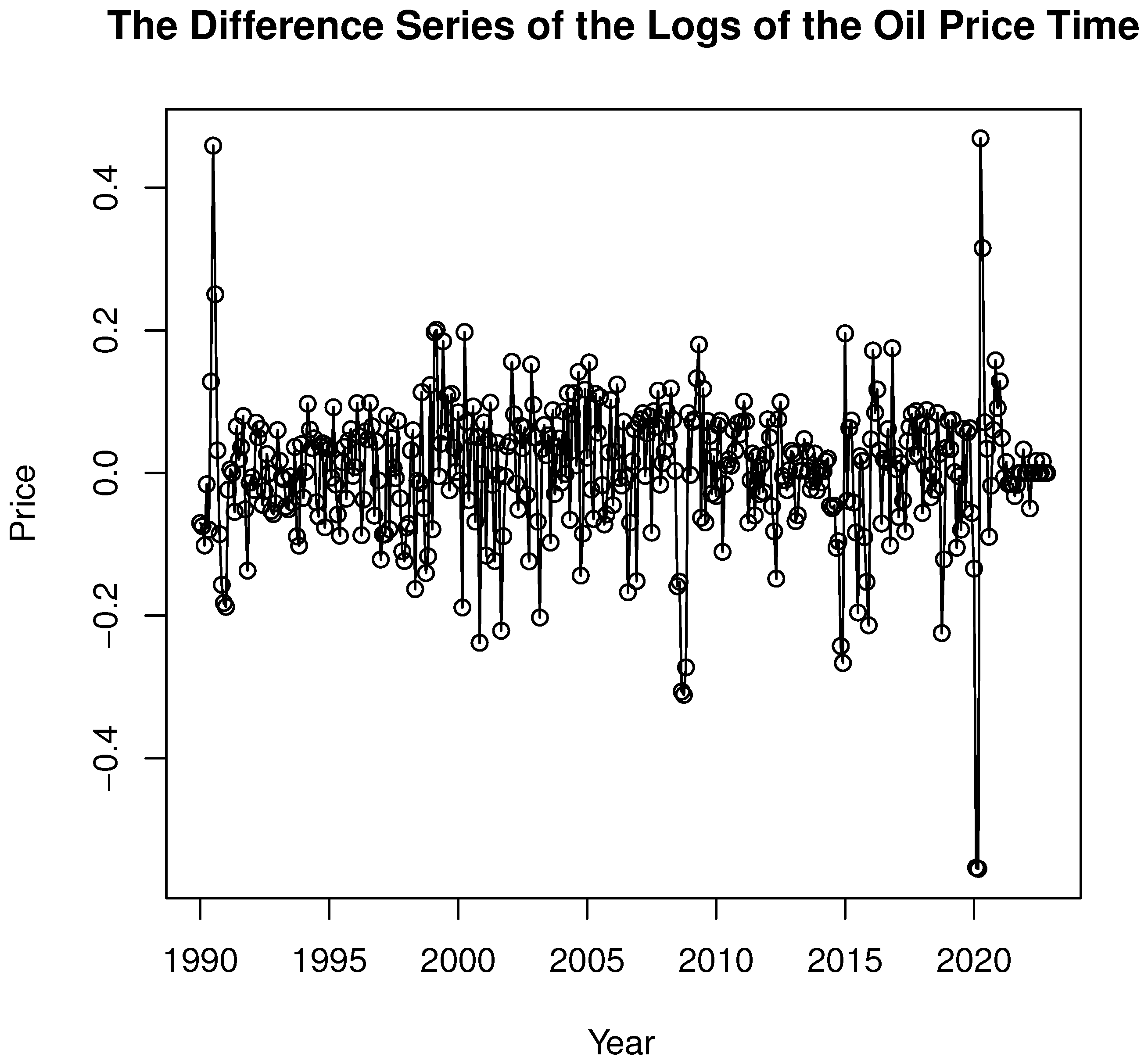
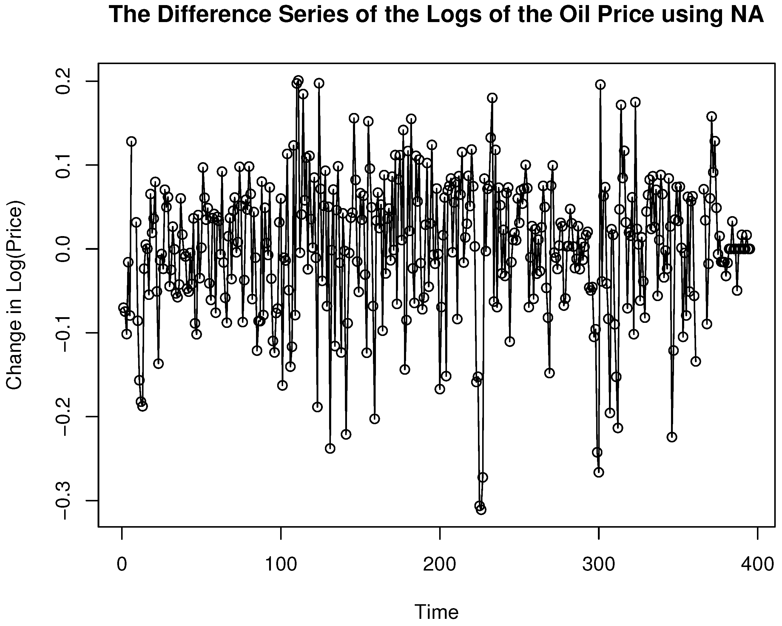
The monthly Brent crude oil spot price $Y_t$ (dollars per barrel) with 396 observations was collected over the period of 01/1990–12/2022. The differenced time series did not have constant variance. Hence, the differenced time series $X_t$ of log(price) was used. The plot of time series in Figure 1 shows several outliers, cases 7, 8, 362, 363, 364, and 365, which create white space in the plot. The outliers near 2020 may be due to COVID-19. These six outliers were replaced by missing values. Hence, if $X_t=log\left(Y_t\right)-log\left(Y_{t-1}\right)$ is the original time series, then $W_t$ is the new time series with $W_t=X_t$ if $X_t$ is not one of the outliers, and $W_t=NA$ if $X_t$ was an outlier, where NA is R notation for missing values. This new technique for handling outliers is useful if the time series software can handle missing values. See Figure 2 for the plot of $W_t$. The auto.arima function was used for model selection and picked an AR(1) model, which appeared to be reasonable from ACF and PACF plots. The new model selection procedure and the Pötscher method both selected an ARMA(1,1) model, which is consistent if the AR(1) model is consistent.

The large sample 95% PI (10) (computed from the 389 values that were not missing) was $[-0.1963,0.1643]$ and contained $371/389=0.9537$ of the 389 $X_t$. If the last nine $X_t$ were omitted, then the large sample 95% PI (10) (computed from the 380 values that were not missing) was $[-0.1965,0.1644]$ and contained all 9 of the future cases $X_{381},\dots ,X_{389}.$ Next we computed the large sample 95% PI (10) using $X_i$ to $X_{i+99}$ for $i=1,\dots ,150$ and determined whether $x_{i+109}$ was in the PI (10 steps ahead, ignoring missing values). This occurred for $139/150=0.927$ of the PIs, and the average PI length was 0.372. Some R code is shown below.

• source("{http://parker.ad.siu.edu/Olive/tspack.txt")
• library(forecast)
• d=read.csv("{http://parker.ad.siu.edu/Olive/BSP.csv")
• d1=diff(log(d$price))
• d1[c(7,8,362,363,364,365)] <- NA
• pricets=ts(d1,frequency=12, start=c(1990,1))
• plot.ts(pricets, main="The Difference Series of the Logs of the Oil Price",
• xlab="Year", ylab="Price",type="o")
• d2 <- d1[-c(7,8,362,363,364,365)]
• locpi(d2)
• d3 <- d2[1:380]
• locpi(d3) #get rolling forecasts
• cov <- 0
• len <- 1:150
• for(i in 1:150){
• dd <- d2[i:(i+99)]
• temp <- locpi(dd)
• yf <- d2[i+109]
• if(temp$LPI <= yf && yf <= temp$UPI)
• cov<-cov+1
• len[i] <- temp$UPI-temp$LPI }

Figure 1. Differenced series of logs of oil price.

Figure 1. Differenced series of logs of oil price.

Figure 2. Differenced series of logs of oil price using NA.

Figure 2. Differenced series of logs of oil price using NA.

For the model selection and PI simulations, there were four error types for the iid $e_t$: (1) N(0,1), (2) $t_5$, (3) $U(-1,1)$, or (4) (EXP(1) − 1), a shifted exponential distribution. All these distributions have mean 0, but the fourth distribution is not symmetric. The 6 time series types were tstype = 1 for an AR(1) model with $\varphi =0.5$, tstype = 2 for an AR(2) model with $\mathit{\varphi }={(0.5,0.33)}^T$, tstype = 3 for an MA(1) model with $\theta =-0.5$, tstype = 4 for an MA(2) model with $\mathit{\theta }={(-0.5,0.5)}^T$, tstype = 5 for an ARMA(3,1) model with $\mathit{\varphi }={(0.7,0.1,-0.4)}^T$ and $\theta =0.1$. Finally, tstype = 6 allows the user to specify $\mathit{\varphi }$ and $\mathit{\theta }$ for an ARMA($p,q$) model with $p\ge 1$, $q\ge 1$, and $p,q\le kmax$, where kmax is the largest value of r for the fitted ARMA($r,r$) models, $r=0,1,\dots ,$ kmax.

Model Selection Simulations

We used the auto.arima function with “AIC”, the Pötscher (1990) [24] method that selects an ARMA($\widehat{r},\widehat{r}$) model, and the new ARMA model selection method given in Section 2.1. In

Table 1. ARMA, proportion of runs where a consistent model was selected; $\varphi =0.4$, $\theta =-0.7$, R AIC for auto.arima; $\widehat{r}$ for the Pötscher method; I for the new method.

n	Dist	R AIC	$\widehat{\mathit{r}}$	I
50	N	0.151	0.561	0.561
200	N	0.239	0.979	0.979
500	N	0.152	1.00	1.00
2000	N	0.249	1.00	1.00
50	t	0.151	0.609	0.609
200	t	0.239	0.944	0.944
500	t	0.109	1.00	1.00
2000	t	0.233	1.00	1.00
50	U	0.153	0.559	0.559
200	U	0.241	0.953	0.953
500	U	0.229	0.982	0.982
2000	U	0.309	1.00	1.00
50	sEXP	0.149	0.569	0.569
200	sEXP	0.241	0.959	0.959
500	sEXP	0.179	0.995	0.995
2000	sEXP	0.263	1.00	1.00

and

Table 2. Proportion of runs where a consistent model was selected; tstype = 5; R AIC for auto.arima; $\widehat{r}$ for the Pötscher method; I for the new method.

n	Dist	R AIC	$\widehat{\mathit{r}}$	I
500	N	0.251	0.381	0.364
800	N	0.279	0.692	0.609
1000	N	0.361	0.648	0.619
1500	N	0.357	0.943	0.832
2000	N	0.514	1.00	0.954
500	t	0.219	0.354	0.324
800	t	0.283	0.654	0.584
1000	t	0.354	0.793	0.739
1500	t	0.359	0.939	0.793
2000	t	0.389	0.969	0.904
500	U	0.219	0.409	0.339
800	U	0.229	0.713	0.680
1000	U	0.324	0.839	0.761
1500	U	0.434	0.964	0.879
2000	U	0.524	0.983	0.963
500	sEXP	0.279	0.362	0.301
800	sEXP	0.323	0.619	0.519
1000	sEXP	0.419	0.774	0.663
1500	sEXP	0.369	0.939	0.889
2000	sEXP	0.394	0.994	0.909

, these methods are denoted by R AIC, $\widehat{r}$, and I, respectively. AIC was used with auto.arima since in the simulations for $n\le 500$, underfitting was much more of a problem than overfitting. The simulations give the proportion of times a consistent model I was selected. Thus $p_I=p_S$ and $q_I\ge q_S$ or $q_I=q_S$ and $p_I\ge p_S$.

For the 6 time series types, searching all 36 models with auto.arima would select a consistent model about 75% to 96% of the time if the true model was AR(p) or MA(q) and n was large (tstype 1 to 4), but it did not perform well for ARMA(1,1) models.

The ARMA models were sensitive to the values of $\mathit{\varphi }$ and $\mathit{\theta }$. For ARMA(1,1) models with ${(\varphi ,\theta )}^T=(0.5,0.2),(0.2,0.1),(0.4,-0.1),(0.6,-0.3),(-0.2,0.6),(-0.4,0.8),(-0.6,1.0),$

$(0.2,-0.5),(0.4,-0.7),(-0.2,-0.1),(-0.4,0.1),(-0.6,0.4),(-0.8,0.6),$ the Pötscher method worked well with $n=1000$, but ${(\varphi ,\theta )}^T=(0.5,-0.5)$ did not. In the simulations, the Pötscher model selection method could work fairly well for n as low as 80, and often worked fairly well for $n=600$, but often much larger sample sizes were needed. The tstype = 5 model needed $n\ge 1500$. Chan, Ling, and Yau (2020) [19] suggested that the Pötscher (1990) [24] method is reliable for $n\ge 1000$. More simulations are presented in Welagedara (2023) [40].

For the simulated ARMA(1,1) time series in Table 1, the Pötscher (1990)  [24] and new methods picked a consistent model in at least 94% of the runs (were reliable) for $n\ge 200$, while auto.arima with AIC picked an inconsistent model in at least 69% of the 1000 runs (was unreliable). Table 2 used the tstype = 5 = ARMA(3,1) model. The new method was fairly reliable for $n\ge 1500$, while auto.arima with AIC picked an inconsistent model in at least 47% of the 1000 runs.

Prediction Intervals after Model Selection

For ease of programming, we used one-step ahead prediction intervals after model selection using the auto.arima function, the GMLE, and $AI{C}_C$. Haile (2022) [41] provided additional prediction intervals and simulations. With 5000 runs, coverages between 0.94 and 0.96 suggest that there is no reason to believe that the nominal coverage is not 0.95. The iid error distributions for $e_t$ were N(0,1), $t_5$, $U(-1,1)$, or (EXP(1) − 1), a shifted exponential distribution. For $h=1$, the asymptotic optimal lengths of the 95% PIs are 3.92, 5.141, 1.9, and 2.996, while the asymptotic lengths of the normal (Chebyshev) nominal 95% PIs are $3.92\sigma$ = 3.92, 5.061, 2.263, and 3.92 for the N(0,1), $t_5$, $U(-1,1)$, and (EXP(1) − 1) distributions, respectively. By Theorem 3, for MA(∞) time series, using iid data formulas, the asymptotic coverages of the nominal 95% Chebyshev intervals for the four error distributions are 0.95, 0.948, 1.00, and 0.948.

Table 3. One-step-ahead PIs after model selection, coverages, and lengths.

n	Dist	Cov/Len	PI (12)	PI (F)	PI (9)
100	N	cov	0.9592	0.9442	0.9476
100		len	4.3214	3.8857	3.9341
100	t5	cov	0.9550	0.9412	0.9434
100		len	5.6747	5.0015	5.0637
100	U	cov	0.9776	0.9842	0.9860
100		len	2.1992	2.2538	2.2819
100	sEXP	cov	0.9540	0.9406	0.9424
100		len	3.7989	3.8504	3.8983
400	N	cov	0.9500	0.9470	0.9476
400		len	3.9990	3.9119	3.9239
400	t5	cov	0.9444	0.9404	0.9412
400		len	5.2364	5.0455	5.0609
400	U	cov	0.9576	0.9988	0.9992
400		len	1.9644	2.2593	2.2662
400	sEXP	cov	0.9578	0.9508	0.9518
400		len	3.2935	3.9047	3.9166
800	N	cov	0.9526	0.9514	0.9520
800		len	3.9445	3.9147	3.9206
800	t5	cov	0.9480	0.9452	0.9456
800		len	5.1604	5.0491	5.0568
800	U	cov	0.9524	0.9994	0.9994
800		len	1.9255	2.2605	2.2640
800	sEXP	cov	0.9438	0.9410	0.9410
800		len	3.1842	3.9147	3.9207

gives some results for nominal 95% PIs. The full model was the ARMA(5,5) model. The true model was an MA(2) model. PIs (9) and (12) were used, as well as the normal (Chebyshev) nominal 95% PI from auto.arima, denoted by (F). Two lines were provided for each distribution-sample size combination. The first line gives the simulated coverage, which tended to be higher than 0.94. The second line gives the average PI length. PIs (9) and (F) were very similar. For $n=800$, the PI lengths and coverages were close to their asymptotic values.

In limited simulations, one-step ahead prediction intervals (12) and the Chebyshev “95%” h-step ahead prediction intervals (10) simulated fairly well after model selection using auto.arima or the Pötscher method. Prediction interval (10) does not depend on model selection. For example, in

Table 4. One-step-ahead PIs after model selection, $\varphi =0.4,\theta =-0.7$.

n	Model Selection Method	Cov/Len	PI (10)	PI (12)	PI (F)
100	A	cov	0.9508	0.9510	0.9380
100	A	len	5.6964	5.6948	5.0013
100	P	cov		0.9574	0.9334
100	P	len		5.9887	4.9387
200	A	cov	0.9476	0.9508	0.9426
200	A	len	5.4792	5.3964	5.0300
200	P	cov		0.9554	0.9432
200	P	len		5.5153	5.0007
400	A	cov	0.9478	0.9514	0.9482
400	A	len	5.3971	5.2408	5.0444
400	P	cov		0.9516	0.9490
400	P	len		5.2918	5.0323

, the true model was an ARMA($0.4,-0.7$) model, the $e_t$ were iid $t_5$, A stands for auto.arima, and P stands for the Pötscher method. PI (10) does not depend on the model selection method; hence, the coverage and length were provided for A but not for P. For PI (12) and PI (F), the coverages and lengths were similar for A and P. Note that PI (12) was slightly longer than PI (10) for P and $n=100,200$. Also, the PI (F) average length is close to the asymptotic length 5.061, while the PI (12) length is not as close to the asymptotically optimal length 5.141.

A random walk or AR(1) model with unit root is $Y_t=Y_{t-1}+e_t$. This time series model is not weakly stationary. The PIs (8) and (10) are valid for AR(1) models with a near unit root, so they may simulate well for the unit root model if the iid errors have $E\left(e_t\right)=0$ and $V\left(e_t\right)={\sigma }_e^2$.

Table 5. One-step-ahead PIs after model selection, random walk, $e_t\sim N(0,1)$.

n	Cov/Len	PI (10)	PI (12)	PI (F)
100	cov	0.9680	0.9672	0.9494
100	len	4.3671	4.4796	3.8887
200	cov	0.9546	0.9528	0.9432
200	len	4.0999	4.1237	3.9036
400	cov	0.9534	0.9508	0.9498
400	len	3.9897	4.0035	3.9129

shows some results for one step ahead PIs when $e_t\sim N(0,1)$ where auto.arima was used.

Some R code is shown below.

• #Table 4, need the source command for tspack and library(forecast)
• arimapisim(n=400,nruns=5000,phi=0.4,theta=-0.7,tstype=6,etype=2,dd=0)
• arimapisim(n=200,nruns=5000,phi=0.4,theta=-0.7,tstype=6,etype=2,dd=0)
• arimapisim(n=100,nruns=5000,phi=0.4,theta=-0.7,tstype=6,etype=2,dd=0)
• #Table 5
• unitrootpisim(n=100,nruns=5000)
• unitrootpisim(n=200,nruns=5000)
• unitrootpisim(n=400,nruns=5000)

3. Discussion

For MA(∞) models, PIs (8) and (10) were proven to have good asymptotic coverage for $h\ge 1$ and to have near optimal asymptotic length for large h. PIs (8) and (10) may be rather long for small h. If the search is restricted to ARMA($k,k$) models, and if $r_S=max(p_S,q_S)\le k_{max}$, then the probability that the ARMA($r_S,r_S$) model is chosen goes to 1 as $n\to \infty$ if BIC is used. Hence (12) is a large sample $100(1-\delta )\%$ PI for $Y_{n+h}$ if the Pötscher method is used.

Heuristically, ARMA and ARIMA model selection is often useful for prediction since the selected submodel tends to have fitted values and residuals that are very highly correlated with those of the full model and hence with those of the unknown “optimal ARIMA($p_S,d,q_S$) model.” Thus, the Chebyshev PI and PI (12) should be similar for the selected model, the ARMA($r_S,r_S$) model, and the ARMA($p_S,q_S$) model, at least for very small and very large values of h. To our knowledge, there is no other explanation for why the Chebyshev PIs simulate well after variable selection.

Consider the usual sample estimators, computed from iid $Y_i$, of population percentiles, mean, variance, and the shorth. Theorem 3 showed that these estimators are consistent estimators of the population quantities, even if the $Y_t$ are from an MA(∞) time series model. This result means that Olive (2013) [33] PIs for multiple linear regression, that use the shorth of the residuals, work even if the errors follow an MA(∞) model, provided that least squares gives a consistent estimator of $\mathit{\beta }$. As shown in Example 2, a useful technique for handling outliers is to replace the outliers with missing values.

The Chebyshev “95%” prediction intervals, such as (9), are useful even after model selection, provided that consistent estimators of ${\mu }_{t+h}$ and ${\sigma }_{t+h}$ are used, but the asymptotic coverage could be between 0.74 and 1.0, depending on the error distribution. PIs (8) and (10), the new PI (12) with $h=1$, and the Chebyshev “95%” h-step ahead prediction intervals simulated fairly well after model selection using auto.arima or the Pötscher method. Remarks 1 and 2 and Section 2.1 help explain why PIs after model selection can perform fairly well if the selected submodel has fitted values and residuals that are very highly correlated with those of a consistent model. Huang et al. (2022) [11] show that the variance estimator and the estimator $\widehat{\mathit{\beta }}$ are still useful even when the model overfits.

Model selection methods that use AIC, BIC, or $AI{C}_C$ tend to be unreliable at selecting a submodel that has a consistent estimator. Using BIC from Equation (6), $k_{max}=p_{max}=q_{max}$, and fitting the ARMA($k,k$) models for $k=0,1,\dots ,k_{max}$ with the Pötscher method had much better performance but still needed $n\ge 600$ to be fairly reliable. For data splitting, suppose the first $n_H$ values of the time series are used to select the ARMA($k_I,k_I)$ model I, and the remaining $n_V=n-n_H$ values for inference. Then, $n_H\ge 600$ and $n_V\ge 20k_I$ should be used. Hence, the time-series length needs to be fairly long, $n\ge 600+20k_{max}$, in order to use data-splitting inference. Much larger values of $n_H$ and $n_V$ are sometimes needed.

There is a large literature on ARIMA time series PIs, especially for AR(p) models, and the bootstrap is often used. Most of the literature assumes the model and order are known, thereby ignoring model selection. See Haile (2022) [41], Hyndman and Athanasopoulos (2018) [39], Lu and Wang (2020) [42], and Pan and Politis (2016)  [43] for references. See Hong, Kuffner, and Martin (2018) [44] for why classical PIs after AIC variable selection do not work. Hyndman and Athanasopoulos (2018, last paragraph of ∮8.8) [39] note that ARIMA-based prediction intervals tend to be too narrow, so actual coverage is less than the nominal coverage. See Bhansali (1981) [45] for the effects of estimating the order of the time series model. Data sets in which future data do not behave like past data are common, and then the prediction intervals tend to perform poorly.

There is a large literature on outlier-anomaly detection in time series. Often, imputation is used, for example, to replace the outlier with the sample mean or median of neighboring values. See Blázquez-García, Conde, Mori, and Lozano (2021) [46] and Welagedara (2023) [40] for references. Replacing outliers with missing values is useful because software methods for handling missing values, including Chebyshev PIs, are widely available. See, for example, Jones (1980) [47].

Plots and simulations were done in R. See R Core Team (2024) [48]. Programs are in the collection of functions tspack.txt. See http://parker.ad.siu.edu/Olive/tspack.txt (accessed on 15 January 2026). The function armamsel1 performs Pötscher (1990) [24] ARMA model selection method, and the function armamsel2 also performs the new ARMA model selection method described in Section 2. The function armasim3 did the simulation for Table 1 and Table 2.

The function locpi gets PI (10). The function locpi2 needs the forecast residuals and finds $[L_n,U_n]$ used in PI (12). One-step-ahead PIs similar to (12) are easy to compute if the one-step-ahead residuals are given by the model selection output. The function onesteppi computes the one-step-ahead PI for seasonal ARIMA(${p,d,q)\times (P,D,Q)}_s$ models with period s, where the six estimated parameters need to be given. The function can handle missing values entered as NA. For Table 3, the function pitsvssim simulates PIs (9) and (12) after model selection using the GMLE with $AI{C}_C$ using the R function auto.arima. Table 5 used the function unitrootpisim.

For Table 4, the functions armapisim and arimapisim compare auto.arima and the Pötscher method for three 1-step ahead methods. The function tspisim compares auto.arima and the Pötscher method for the normal Chebyshev h-step ahead PIs. These three functions would often fail if 5000 runs were used.