Max–Min Transitive Closure of Randomly Generated Fuzzy Matrix: Bernoulli and Classical Probabilistic Models

Abstract

A randomly generated fuzzy matrix refers to a fuzzy matrix in which the values of elements belong to the sample space of a [0,1]-random variable that follows a certain probability distribution. This paper studies the max–min transitive closure of two-type randomly generated fuzzy matrices: Bernoulli and classical probabilistic models. By introducing the concept of superposed fuzzy matrices, we investigate the probability distribution of the transitive closure of randomly generated fuzzy matrices for two probabilistic models. First, we presented the arithmetic operation rules for the superposed fuzzy relations. The expected value of the randomly generated Bernoulli fuzzy matrix transition closure was studied. A direct calculation method for the randomly generated fuzzy matrix transitive closure of the classical probability model was provided. Finally, the errors between the direct calculation method and the traditional transitive closure calculation method were compared.

1. Introduction

Fuzzy matrices have found widespread application in fields such as fuzzy logic reasoning, fuzzy discrete event systems, and expert systems. The elements of a fuzzy matrix typically represent fuzzy relations or membership degrees between elements of a set. However, in many real-world problems, the relationships between some elements are not directly apparent but are indirectly connected through others. Therefore, it is necessary to reveal potential indirect relations between elements through the transitive closure, which better supports reasoning and decision-making tasks. Given an $N\times N$ fuzzy matrix $\mathbf{R}$, its transitive closure can be computed using the following formula:

$${\mathbf{R}}^{+}=\mathbf{R}\cup {\mathbf{R}}^2\cup \cdots \cup {\mathbf{R}}^N.$$

(1)

More specifically, if matrix A represents a fuzzy relation between elements, the transitive closure of A is computed by repeatedly applying the relation (min–max operations) until no further updates occur, thus capturing all possible indirect relations. This is similar to the classical definition of transitive closure in binary relations, but extended to fuzzy sets where degrees of relation are considered rather than binary values.

The time complexity for computing the transitive closure of an N-dimensional fuzzy matrix through Equation (1) is $\mathcal{O}\left(N^5\right)$[1]. Many algorithms have since been proposed to improve the efficiency of transitive closure computation. For instance, the well-known Warshall algorithm can compute the transitive closure of a fuzzy matrix in $\mathcal{O}\left(N^3\right)$ time [2], while for a fuzzy similarity matrix, its transitive closure can be obtained in $\mathcal{O}\left(N^2\right)$ time [3].

1.1. Motivations

There are two main motivations.

1.1.1. Fuzzy Relation in Probabilistic Uncertain Environment

In practical applications, the acquisition of fuzzy relations is often influenced by various factors that can introduce inconsistency. These factors include environmental noise, observational errors, and the subjective judgments of experts. Such uncertainties complicate the determination of precise fuzzy relations, making it essential to adopt a probabilistic approach to better reflect the inherent variability in the data. For instance, consider the case of assessing whether a 60-year-old individual qualifies as “elderly”. Different experts may hold varying opinions based on their experiences, biases, and the context in which the assessment occurs. In this scenario, 60% of experts might assert that the individual’s membership degree to the category “elderly” is 0.7, indicating a strong belief that the person belongs to this category. Meanwhile, 30% of experts may argue for a slightly lower membership degree of 0.6, reflecting a more cautious stance, while the remaining 10% might consider the membership degree to be only 0.5, suggesting that they see the individual as only somewhat fitting the definition of “elderly”. This divergence of opinions illustrates that the membership degree is not merely a fixed fuzzy number; rather, it can be seen as a variable that follows a probability distribution. This insight leads us to reconsider how we model fuzzy relations in light of expert judgment variability and uncertainty. By incorporating probabilistic elements into our models, we can better capture the nuances of real-world situations and enhance the robustness of our fuzzy reasoning frameworks.

1.1.2. Transitive Closure of Large-Scale Fuzzy Matrices

In addition, the characteristics of probability distributions often become more pronounced in larger-scale problems. The time complexity of traditionally computing fuzzy matrices is $O\left(N^3\right)$ [2], which is acceptable for small fuzzy matrices. However, for large or extremely large fuzzy matrices, the computational demands increase significantly, leading to longer processing times and increased resource consumption. This raises an important question: can we use the properties of probability to uncover a direct functional mapping between large fuzzy matrices and their transitive closures? By establishing such a mapping, we could potentially simplify the process of computing the transitive closure, thereby improving efficiency. This approach would allow us to bypass some of the computational complexities associated with traditional methods for calculating transitive closures, enabling faster and more effective analysis of large-scale fuzzy matrices in real-world applications, such as model checking [4,5].

1.1.3. AI for Fuzzy Systems

Fuzzy systems play a crucial role in the field of artificial intelligence, providing a framework for handling uncertainty and imprecision in data. However, developing an effective learning algorithm for large-scale fuzzy systems presents significant challenges that are both resource-intensive and time-consuming. One of the main difficulties arises during the development phase, where we often need to randomly generate a large fuzzy matrix to serve as a model for the system for generating samples [6,7], conducting learning processes, and performing tests. For instance, in the context of addressing the reachability problem within fuzzy systems [8,9], the learning process necessitates the computation of the transitive closure of these large fuzzy matrices. This computation is inherently demanding and can consume a substantial amount of time, particularly as the size of the matrix increases. Additionally, the learning process requires a considerable number of samples and epochs to achieve satisfactory results. Each sample involves significant computational effort, which can lead to a bottleneck in the learning process. As the number of samples increases, the total time required for learning can become prohibitive, rendering the entire process impractical for large-scale applications. This situation poses a significant challenge for researchers and practitioners who aim to implement fuzzy systems in real-world scenarios, where efficiency and speed are paramount.

Given these challenges, there is a pressing need for innovative approaches to streamline the learning process for large-scale fuzzy systems. By optimizing the generation and computation of the transitive closure for fuzzy matrices, we can accelerate the learning process, making it more feasible for practical implementation in artificial intelligence.

1.2. Main Ideas

To quantify the probabilistic uncertainty of fuzzy relations between elements in a set, inspired by the concept of superposition in quantum mechanics [10,11], we propose the concept of “superposed fuzzy relation (SFR)”. Superposed fuzzy relations map two elements of a set into a superposed state of membership degrees. The superposed membership state indicates that the relationship between two elements simultaneously exists at multiple possible membership degrees. By observing a superposed fuzzy relation, the superposed membership degree collapses probabilistically into a definite membership degree. For example, continuing with the 60-year-old case, a person’s membership degree to the “elderly” category is simultaneously in a superposed state of 0.7, 0.6, and 0.5. After consulting an expert’s opinion (i.e., making an observation/measurement), the superposed membership degree has a 60% chance of collapsing to 0.7, a 30% chance of collapsing to 0.6, and a 10% chance of collapsing to 0.5.

The fuzzy relations between elements in a set can be represented by a fuzzy matrix. Similarly, a matrix induced by superposed fuzzy relations is referred to as a “superposed fuzzy matrix (SFM)”. Intuitively, the elements in a superposed fuzzy matrix are variables following a certain probability distribution (i.e., they are in a superposed membership state). By measuring a superposed fuzzy matrix, it also collapses into a fuzzy matrix. We refer to the fuzzy matrix obtained after measuring the superposed fuzzy matrix as a “randomly generated fuzzy matrix (RGFM)”. Therefore, a randomly generated fuzzy matrix is also a fuzzy matrix.

Based on superposed versions of these fuzzy relations, this paper studies the relationship between randomly generated fuzzy matrices and their max–min transitive closures. First, we define the arithmetic operations of superposed fuzzy relations, including the “∧” and “∨” operations. We provide the calculation formula for the superposed transitive closure induced by superposed fuzzy relations. Next, we study the probability distributions of the superposed transitive closures of finite-dimensional superposed fuzzy matrices with Bernoulli-type, uniform distribution (classical probabilistic model). We derive the expected value formula for the superposed transitive closure of superposed fuzzy matrices. Then, we explore the limit properties of superposed fuzzy matrices, showing that the expected value of the power limit of a superposed fuzzy matrix converges to the maximum of the random variables.

1.3. Related Work

To the best of our knowledge, this paper introduces the concept of probability fuzzy matrices for the first time. It is important to distinguish this from fuzzy probability matrices, also known as fuzzy Markov matrices [12,13,14]. Probability fuzzy matrices are constructed based on fuzzy probability theory [15], where the element values represent probabilities, but these probabilities exhibit fuzzy uncertainty. Specifically, in fuzzy probability theory, the probability of an event occurring is no longer represented by a specific numerical value but is described through fuzzy sets. Intuitively, “probability fuzzy” means that different fuzzy numbers appear with different probabilities. In contrast, “fuzzy probability” refers to the representation of probabilities in the form of fuzzy sets.

1.4. Structures of the Paper

The arrangement of the remaining sections of this paper is as follows. Section 2 introduces the basic concepts and arithmetic operations related to superposed fuzzy relations. Section 3 presents the probability distribution of the transitive closure of discrete superposed fuzzy matrices. Section 4 investigates the limiting properties of superposed fuzzy matrices. Appendix A provides an efficient approximation algorithm for large probabilistic fuzzy matrices and conducts a performance analysis. The final section illustrates the effectiveness of the proposed methods through a case study.

2. Superposed Fuzzy Theory

In this section, we will introduce the basic concepts and arithmetic operations of superposed fuzzy relations, as well as the matrix form of superposed fuzzy relations: superposed fuzzy matrices.

Superposed fuzzy relation (FSR) is a concept used to describe the probabilistic fuzzy relations between elements in a set, inspired by the idea of superposition in quantum mechanics [10,11]. In a traditional fuzzy matrix, the fuzzy relation between elements is usually represented by a definite membership degree. However, in superposed fuzzy relation, the fuzzy relation between two elements is not a fixed membership degree but a superposition state of multiple possible membership degrees. Specifically, superposed fuzzy relation maps the fuzzy relationship between two elements to a combination of several membership degrees, meaning that a membership degree can simultaneously exist in multiple membership degrees. Without further observation, these membership degrees remain uncertain, and their possible values are described probabilistically. When a superposed fuzzy relation is observed, the superposed membership degree collapses probabilistically into a definite value.

This concept is particularly useful when dealing with situations where a single membership degree cannot be determined due to inconsistencies or uncertainties, such as when membership degrees are influenced by conflicting expert opinions, environmental noise, or data errors. Superposed fuzzy relation allows for a more precise quantification and description of uncertainties, thereby providing better support for fuzzy reasoning and decision-making tasks. Importantly, superposed fuzzy relation is also a very good mathematical tool for calculating the probability distribution of elements in transitive closures of randomly generated fuzzy matrices.

2.1. Basic Assumptions of Quantum Mechanics

First, it is essential to briefly introduce the basic assumptions of quantum mechanics [10,11], as they play a significant role in our understanding of the methods proposed in this paper.

In quantum mechanics, superposition refers to a quantum system’s ability to exist in multiple states simultaneously, represented as a linear combination of basis states by using Dirac symbols, as follows:

$$|\psi \rangle =c_1|a_1\rangle +c_2|a_2\rangle +\dots +c_n|a_n\rangle .$$

(2)

Here, $|\psi \rangle$ denotes the system’s state, $|a_i\rangle$ is the basis states, and $c_i$ is complex coefficients indicating the weight of each state. When a measurement is performed on the quantum system, its state collapses to a specific basis state. The result of the measurement depends on the weights in the superposition, with the probability of obtaining state $|a_i\rangle$ given by $Pr\left(a_i\right)={\left|c_i\right|}^2$.

Thus, measurement is crucial in quantum mechanics as it transforms the superposition into a definite state. After measurement, the superposition collapses to a specific state. This means that the quantum system transitions from a superposition to a definite outcome corresponding to the measurement result. Additionally, quantum entanglement is a fundamental property of quantum states; however, it is not relevant to this paper and will not be discussed here. Together, these concepts form the fundamental framework of quantum mechanics.

2.2. Superposed Fuzzy Relations

In this subsection, we generalize the concept of fuzzy relations to incorporate probabilistic uncertainty by allowing membership degrees to follow a probability distribution. That is, a fuzzy relation is no longer a single membership degree but a discrete random variable over all possible membership degrees. The sample space of this random variable can be derived from a lattice or other methods for obtaining membership degrees; however, such methods are beyond the scope of this work.

Definition 1 

(Discrete Random Variables). Let $X=x_1,x_2,\cdots ,x_n$ with an order $x_1\le x_2\le \cdots \le x_n$ be a discrete random variable and follow a probability distribution $f_X\left(x\right)\triangleq Pr(X=x)$; write

$$X\sim f_X\left(x\right),$$

(3)

where ${\sum }_{x}f\left(x\right)=1$.

In the case where the random variable X is clear, we can write $f_X\left(x\right)$ as $f\left(x\right)$.

A superposed fuzzy relation allows a fuzzy relationship to exist over all possible membership degrees simultaneously, each weighted by its corresponding probability. Formally, it is a set of pairs consisting of a membership degree and its corresponding probability.

Definition 2 

(Superposed Fuzzy Relations). Let $X\sim f\left(x\right)$ be a discrete random variable. For two finite sets A and B, the superposed fuzzy relation $R_f$ over the Cartesian product $A\times B$ is defined as a function, as follows:

$$R_f:A\times B\to \{\langle x,f\left(x\right)\rangle \mid x\in X\}.$$

(4)

Alternatively, using the Dirac notation, it can be expressed as

$$R_f:A\times B\to f\left(x_1\right)|x_1\rangle \oplus f\left(x_2\right)|x_2\rangle \oplus \cdots \oplus f\left(x_n\right)|x_n\rangle ,$$

(5)

where $x_1,x_2,\dots ,x_n\in X$ and ${\sum }_{k=1}^{n}f\left(x_k\right)=1$. We call $f\left(x_1\right)|x_1\rangle \oplus f\left(x_2\right)|x_2\rangle \oplus \cdots \oplus f\left(x_n\right)|x_n\rangle$ the “superposed membership degree” and $f\left(x\right)$ the “probability distribution” for superposed fuzzy relation $R_f$.

If $f\left(x\right)=1$ for a specific element $x\in X$, the superposed fuzzy relation $R_f$ reduces to a fuzzy relation R. Thus, a classical fuzzy relation is a special case of a superposed fuzzy relation.

Since the definition of a superposed fuzzy relation is independent of the elements in the set $A\times B$, it can be concisely represented as

$$R_f=\underset{k=1}{\overset{n}{⨁}}f\left(x_k\right)|x_k\rangle .$$

(6)

In the following, we will alternate between the notations $R_f$ and $R_f(a,b)$ as needed for clarity.

Example 1. 

Consider two finite sets, $A=\{a,b\}$ and $B=\{c,d\}$, and a finite lattice, $L=\{0.4,0.5,0.6\}$. Let the random variable $X=\{0.4,0.5,0.6\}$ follow the distribution, as follows:

$$f\left(x\right)=\left\{\begin{array}{cc}\mathbf{0.2},\hfill & \mathrm{if}x=0.4,\hfill \\ \mathbf{0.3},\hfill & \mathrm{if}x=0.5,\hfill \\ \mathbf{0.5},\hfill & \mathrm{if}x=0.6.\hfill \end{array}\right.$$

(7)

Here, bold values denote probabilities, while non-bold values denote membership degrees. Then, the superposed fuzzy relation $R_f$ over $A\times B$ can be expressed as

$$R_f(a,c)=R_f(a,d)=R_f(b,c)=R_f(b,d)=\mathbf{0.2}|0.4\rangle \oplus \mathbf{0.3}|0.5\rangle \oplus \mathbf{0.5}|0.6\rangle .$$

(8)

This means that, for each element of $A\times B$, the membership between them is simultaneously 0.4, 0.5, and 0.6 with a probability of 0.2, 0.3, and 0.5, respectively. If $f\left(0.4\right)=1$ and $f\left(0.5\right)=f\left(0.6\right)=0$, the superposed fuzzy relation reduces to a classical fuzzy relation, as follows:

$$R_f(a,c)=\mathbf{1}|0.4\rangle \oplus \mathbf{0}|0.5\rangle \oplus \mathbf{0}|0.6\rangle \Rightarrow R(a,c)=0.4.$$

(9)

Note that, in this example, we construct the set of possible values of the random variable as a finite lattice to facilitate the definition of operations such as minimum, maximum, and transitive closures. In fact, the range of values for random variables is not constrained by the source lattice.

In quantum mechanics, a quantum system exists in a superposition of multiple states. To obtain information about a quantum system, quantum measurement is required. However, after a measurement, the quantum system collapses into a specific quantum state. Similarly, superposed fuzzy relations also require such “measurement” to obtain information about the superposition relation. We can refer to a measurement as an experiment, a test, or even a consultation, depending on the application context. After a measurement, the superposed fuzzy relation probabilistically collapses into a specific membership degree. Formally, we have the following definition of measurement.

Definition 3 

(Measurement). A measurement $\mathbf{M}$ over a superposed fuzzy relation $R_f$ is a function as follows:

$$\mathbf{M}:R_f\to X.$$

(10)

After a measurement, the relation $R_f$ collapses to the value $x_k$ with probability $f\left(x_k\right)$, i.e.,

$$f\left(x_k\right)=Pr[\mathbf{M}\left(R_f\right)=x_k],$$

(11)

where Pr is a probability measure.

Similar to expectation in probability theory, we can define the average membership degree for a superposed fuzzy relation, which we refer to as the expectation.

Definition 4 

(Expectation). The expectation of a superposed fuzzy relation $R_f$ is a function $\mathbf{Exp}:R_f\to [0,1]$ defined as

$$\mathbf{Exp}\left[R_f\right]=\sum _{k=1}^{n}f\left(x_k\right)x_k.$$

(12)

2.3. Arithmetic Operations

For two superposed fuzzy relations, similar to fuzzy relations, there are operations of taking the maximum and taking the minimum. Note that, after performing arithmetic operations on two superposed fuzzy relations, the result is still a fuzzy superposition relation unless subjected to a measurement process. In what follows, we formally define the min and max operations for two given superposed fuzzy relations.

Definition 5 

(Min–Max Operators). For two superposed fuzzy relations, $R_f$ and $R_g$, the min–max operator “$\wedge /\vee$” is defined as

$$R_f\wedge R_g=\underset{k=1}{\overset{n}{⨁}}\left[\sum _{\begin{array}{c}1\le i,j\le n\\ x_i\wedge x_j=x_k\end{array}}f\left(x_i\right)g\left(x_j\right)\right]|x_k\rangle .$$

(13)

$$R_f\vee R_g=\underset{k=1}{\overset{n}{⨁}}\left[\sum _{\begin{array}{c}1\le i,j\le n\\ x_i\vee x_j=x_k\end{array}}f\left(x_i\right)g\left(x_j\right)\right]|x_k\rangle .$$

(14)

This operation computes the component-wise minimum/maximum of two fuzzy superposition relations, accumulating contributions that result in the same basis element $|x_k\rangle$.

The following proposition provides an alternative, more compact representation of the individual probabilities for each basis element $|x_k\rangle$ in the outcome.

Proposition 1. 

The following equation gives a more compact representation of probability for $|x_k\rangle$, $k=1,2,\dots ,n$.

$$\sum _{\begin{array}{c}1\le i,j\le n\\ x_i\wedge x_j=x_k\end{array}}f\left(x_i\right)g\left(x_j\right)=f\left(x_k\right)\sum _{j=k}^{n}g\left(x_j\right)+g\left(x_k\right)\sum _{i=k}^{n}f\left(x_i\right)-f\left(x_k\right)g\left(x_k\right);$$

(15)

$$\sum _{\begin{array}{c}1\le i,j\le n\\ x_i\vee y_j=x_k\end{array}}f\left(x_i\right)g\left(x_j\right)=f\left(x_k\right)\sum _{j=1}^{k}g\left(x_j\right)+g\left(x_k\right)\sum _{i=1}^{k}f\left(x_i\right)-f\left(x_k\right)g\left(x_k\right).$$

(16)

The proof is placed in Appendix A.1.

In fact, Equations (15) and (16) are closely related to the distributions of $min(X,Y)$ and $max(X,Y)$, respectively, where X and Y are two independent discrete variables.

Definition 6 

(Min–Max Power). Consider a superposed fuzzy relation $R_f$; its min m-power, denoted by $R_f^{\wedge m}$, is defined as

$$R_f^{\wedge m}=\underset{m\mathit{times}{R}_f}{\underbrace{R_f\wedge R_f\wedge \cdots \wedge R_f}},$$

(17)

and its max m-power, denoted by $R_f^{\vee m}$, is defined as

$$R_f^{\vee m}=\underset{m\mathit{times}{R}_f}{\underbrace{R_f\vee R_f\vee \cdots \vee R_f}}.$$

(18)

2.4. Matrix Representation

In this section, we will present the transitive closure of superposed fuzzy relations. Similar to fuzzy relations, superposed fuzzy relations also have corresponding matrix representations, called superposed fuzzy matrices.

2.4.1. Superposed Fuzzy Matrix

If $A=\{a_1,a_2,\cdots ,a_m\}$ and $B=\{b_1,b_2,\cdots ,b_n\}$ are finite, the superposed fuzzy relation $R_f$ over $A\times B$ can be represented by a $m\times n$ matrix ${\mathbf{R}}_f$ and

$${\mathbf{R}}_f(i,j)=R_f(a_i,b_j)$$

(19)

for any $1\le i\le m$, $1\le j\le n$. We call ${\mathbf{R}}_f$ the f-type “superposed fuzzy matrix”. Once again, the superposed fuzzy relation is independent of the elements in the set $\Omega$, i.e., $R_f({\omega }_i,{\omega }_j)=R_f$ for any $1\le i,j\le |\Omega |$. Therefore, we could also write a superposed fuzzy matrix as

$${\mathbf{R}}_f={\left[R_f\right]}_{m\times n}.$$

(20)

When the superposed fuzzy relations are represented as matrices, the corresponding operations also follow max–min fuzzy composition rules. Consider two superposed fuzzy relations $R_f$ over $A\times B$ and $R_g$ over $B\times C$. We define superposed fuzzy relation $R_f\circ R_g$ over $A\times C$ as follows:

$$R_f\circ R_g(a,c)=\underset{b\in B}{max}\left[R_f(a,b)\wedge R_g(b,c)\right],\forall (a,c)\in A\times C.$$

(21)

2.4.2. Superposed Transitive Closure

Consider a superposed fuzzy relation $R_f$ over the finite set $\Omega$. We can inductively define the m-th power of its superposed fuzzy matrix ${\mathbf{R}}_f$, as follows:

$${\mathbf{R}}_f^m={\mathbf{R}}_f^{m-1}\circ {\mathbf{R}}_f$$

(22)

for $m\ge 2$ and ${\mathbf{R}}_f^1={\mathbf{R}}_f$. From the commutativity and associativity of max and t-modules, as well as the distributive law of t-modules over max, we can derive another definition for the m-th power of a superposed fuzzy matrix ${\mathbf{R}}_f$ over $\Omega$, as follows:

$${\mathbf{R}}_f^m(s,t)=\underset{u_1,u_2,\cdots ,u_{m-1}\in \Omega }{max}\left[{\mathbf{R}}_f(s,u_1)\wedge {\mathbf{R}}_f(u_1,u_2)\wedge \cdots \wedge {\mathbf{R}}_f(u_{m-1},t)\right]$$

(23)

The transitive closure of $N\times N$ superposed fuzzy matrix ${\mathbf{R}}_f$ is defined as follows:

$${\mathbf{R}}_f^{+}={\mathbf{R}}_f\vee {\mathbf{R}}_f^2\vee \cdots \vee {\mathbf{R}}_f^N.$$

(24)

Proposition 2. 

For an $N\times N$ superposed fuzzy matrix ${\mathbf{R}}_f$, its superposed transitive closure is

$${\mathbf{R}}_f^{+}(i,j)=\underset{m=1}{\overset{N}{\bigvee }}{\left(R_f^{\wedge m}\right)}^{\vee N^{m-1}}$$

(25)

for any $1\le i,j\le N$.

The proof is placed in Appendix A.2.

2.4.3. Randomly Generated Fuzzy Matrices

Let $\mu$ and $\sigma$ denote the functions of calculating the mean and variance of the elements of $N\times N$ matrix $\mathbf{R}$, respectively, i.e., $\mu \left(\mathbf{R}\right)={\displaystyle \frac{1}{N^2}}{\sum }_{i,j}\mathbf{R}(i,j)$, $\sigma \left[\mathbf{R}\right]={\displaystyle \frac{1}{N^2-1}}{\sum }_{i,j}{|\mathbf{R}(i,j)-\mu \left(\mathbf{R}\right)|}^2$.

Definition 7 

(Fair Measurement). Consider a superposed fuzzy matrix ${\mathbf{R}}_f={\left[R_f\right]}_{N\times N}$. If a measurement $\mathbf{M}$ satisfies

• $\mu \left[\mathbf{M}\left({\mathbf{R}}_f\right)\right]\approx \mathbf{Exp}\left[R_f\right]$,
• $\sigma \left[\mathbf{M}\left({\mathbf{R}}_f\right)\right]\approx \mathbf{Var}\left[R_f\right]$,

then we call $\mathbf{M}$ a “fair measurement” for ${\mathbf{R}}_f$; write $\widehat{\mathbf{M}}$.

Definition 8 

(Randomly Generated Fuzzy Matrices). If a fuzzy matrix $\mathbf{R}$ is obtained by measuring fairly a superposed fuzzy matrix ${\mathbf{R}}_f$, then we call $\mathbf{R}$ a “randomly generated fuzzy matrix”. Formally,

$$\mathbf{R}=\widehat{\mathbf{M}}\left({\mathbf{R}}_f\right).$$

(26)

Since the randomly generated fuzzy matrix is the result of fair measurement, we can also call the randomly generated fuzzy matrix the “fair measurement fuzzy matrix”.

3. Transitive Closure of Superposed Fuzzy Matrices

Extensive experimental results indicate that the probability distribution of a superposed fuzzy matrix is closely related to that of its transitive closure. This section begins with the simplest case—Bernoulli-type superposed fuzzy matrix—and explores the probability distribution of its superposed transitive closure. Interestingly, the expected value of the superposed transitive closure of any discrete superposed fuzzy matrix tends to converge to the maximum value of the random variables.

3.1. Bernoulli-Type Superposed Fuzzy Matrices

Recall a Bernoulli trial: the probability of failure is $1-p$, and the probability of success is p. In this paper, we modify the trial outcome to two possible membership degrees, where the probability of obtaining membership degree $x_1$ is $1-p$, and the probability of obtaining membership degree $x_2$ is p.

Consider a random variable $X=\{x_1,x_2\}$ with $x_1\le x_2$ and a superposed fuzzy relation $R_f$ over the set $\Omega$, where the probability distribution function

$$f\left(x\right)=\left\{\begin{array}{cc}1-p,\hfill & \mathrm{if}x=x_1,\hfill \\ p,\hfill & \mathrm{if}x=x_2,\hfill \end{array}\right.$$

(27)

where $p\in [0,1]$. Then $R_f$ is called “Bernoulli(-type) superposed fuzzy relation”. For simplicity, we write the Bernoulli superposed fuzzy relation as

$$B_p=(1-p)|x_1\rangle \oplus p|x_2\rangle .$$

(28)

Here, $B_p$ is the short form of $B_p(a,b)$ for any $a,b\in \Omega$. Note that this abbreviation originates from the fact that superposed fuzzy relations are independent of the elements within the set $\Omega$.

Proposition 3. 

Consider the two Bernoulli superposed fuzzy relations $B_p=(1-p)|x_1\rangle \otimes p|x_2\rangle$ and $B_q=(1-q)|x_1\rangle \otimes q|x_2\rangle$. We have

$$\begin{array}{}\mathrm{(29)}& \hfill B_p\wedge B_q& =& (1-pq)|x_1\rangle \oplus pq|x_2\rangle ,\hfill \mathrm{(30)}& \hfill B_p\vee B_q& =& (1-p)(1-q)|x_1\rangle \oplus (p+q-pq)|x_2\rangle .\hfill \end{array}$$

The proof is based on Proposition 1 and omitted here.

Note that $p+q-pq\ge p$ and $p+q-pq\ge q$. This means that the “∧” operation will bias the distribution of the superposed fuzzy relations towards the smaller value, and the “∨” operation will bias the distribution towards the larger value. These are also the expected results.

Proposition 4. 

For a Bernoulli superposed fuzzy relation $B_p$, its max–min m-th power can be calculated by the following equations, respectively:

$$B_p^{\vee m}={(1-p)}^m|x_1\rangle \oplus [1-{(1-p)}^m]|x_2\rangle ,$$

(31)

$$B_p^{\wedge m}=(1-p^m)|x_1\rangle \oplus p^m|x_2\rangle .$$

(32)

The proof is placed in Appendix A.3.

Next, we will present the probability distribution of the (superposed) transitive closure of Bernoulli superposed fuzzy matrices.

Theorem 1. 

For a Bernoulli superposed fuzzy matrix ${\mathbf{B}}_p={\left[B_p\right]}_{N\times N}$, where $B_p=(1-p)|x_1\rangle \oplus p|x_2\rangle$, its transitive closure is

$$B_p^{+}=\prod _{i=1}^N{(1-p^i)}^{N^{i-1}}|x_1\rangle \oplus \left[1-\prod _{i=1}^N{(1-p^i)}^{N^{i-1}}\right]|x_2\rangle .$$

(33)

The proof is placed in Appendix A.4.

Through Theorem 1, we can see that the probability distribution of the transitive closure of the Bernoulli superposed fuzzy matrix exhibits a strong bias toward larger values due to the presence of the double exponent. This phenomenon becomes more validated as the matrix dimension increases. Intuitively, with the growth of the matrix dimension, the transitive closure gradually absorbs the smaller values in the original fuzzy matrix, leaving only the larger ones. This is an expected result. We illustrate this phenomenon with an example.

Example 2. 

For a Bernoulli superposed fuzzy relation, $R_p=(1-p)|0.2\rangle \oplus p|0.8\rangle$ with $p=0.5$. Its superposed fuzzy matrix is ${\mathbf{R}}_p={\left[R_p\right]}_{N\times N}$ (N=5), as follows:

$${\mathbf{R}}_p=\left(\begin{array}{ccccc}{R}_p& R_p& R_p& R_p& R_p\\ R_p& R_p& R_p& R_p& R_p\\ R_p& R_p& R_p& R_p& R_p\\ R_p& R_p& R_p& R_p& R_p\\ R_p& R_p& R_p& R_p& R_p\end{array}\right).$$

(34)

Consider the probabilistic fuzzy matrix $\mathbf{R}=\widehat{\mathbf{M}}\left[{\mathbf{R}}_p\right]$, as follows:

$$\widehat{\mathbf{M}}\left({\mathbf{R}}_p\right)=\mathbf{R}=\left(\begin{array}{ccccc}0.8& 0.8& 0.8& \mathbf{0.2}& 0.8\\ 0.8& \mathbf{0.2}& \mathbf{0.2}& \mathbf{0.2}& 0.8\\ 0.8& \mathbf{0.2}& 0.8& \mathbf{0.2}& \mathbf{0.2}\\ \mathbf{0.2}& 0.8& 0.8& \mathbf{0.2}& 0.8\\ \mathbf{0.2}& 0.8& \mathbf{0.2}& 0.8& \mathbf{0.2}\end{array}\right).$$

(35)

Then we have

$${\left[\widehat{\mathbf{M}}\left({\mathbf{R}}_p\right)\right]}^{+}={\mathbf{R}}^{+}=\left(\begin{array}{ccccc}0.8& 0.8& 0.8& 0.8& 0.8\\ 0.8& 0.8& 0.8& 0.8& 0.8\\ 0.8& 0.8& 0.8& 0.8& 0.8\\ 0.8& 0.8& 0.8& 0.8& 0.8\\ 0.8& 0.8& 0.8& 0.8& 0.8\end{array}\right).$$

(36)

In this example, we examine how the proportions of elements (0.8 and 0.2) in the transitive closure of a fuzzy matrix evolve as the size increases. The matrix is generated using a probabilistic mapping, where each element is either 0.8 with a probability of p or 0.2 with a probability of $1-p$, where p is a predefined threshold probability $p=0.05$ in the following. The proportion of 0.8 and 0.2 elements in the transitive closure is recorded for different fuzzy matrix sizes (N), ranging from 10 to 200.

The results, illustrated in Figure 1, show that as the size of a fuzzy matrix increases, the relative proportions of these elements converge towards distinct values. We can see that even though the proportion of 0.8 elements in the initial fuzzy matrix is very small (only 5%), the proportion of 0.8 in the transitive closure of the fuzzy matrix increases significantly and approaches 1 as the matrix size grows. Meanwhile, the proportion of 0.2 decreases significantly, with its occurrence probability approaching 0. This result confirms the correctness of Theorem 1. We also draw an accurate probability distribution function curve in Figure 1, i.e., Equation (33). It can be seen that it is almost consistent with the simulation results. This error is due to randomness in the computer.

Next, we will calculate the expected value of the superposed transitive closure of the Bernoulli-type superposed fuzzy matrix.

Theorem 2. 

Consider a Bernoulli-type superposed fuzzy matrix ${\mathbf{B}}_p={\left[B_p\right]}_{N\times N}$, where $B_p=(1-p)|x_1\rangle \otimes p|x_2\rangle$, $p\in [0,1]$. Then the expectation of its superposed transitive closure $B_p^{+}$ is

$$\mathbf{Exp}\left[B_p^{+}\right]=x_2-\prod _{i=1}^N{(1-p^i)}^{N^{i-1}}(x_2-x_1).$$

(37)

The proof is obtained by routine calculation based on Equation (12).

It can be observed that the expected value tends toward the maximum value because the second term of Equation (37) becomes a negligible number when N is large. The expected value plays a crucial role in the approximation algorithm for large-scale probabilistic fuzzy matrix transitive closures discussed in the following.

3.2. Classical Probability Superposed Fuzzy Matrices

 Theorem 3.

Let $X\sim f\left(x\right)$ be a discrete random variable. Suppose that $R_f={⨁}_{k=1}^{n}f\left(x_k\right)|x_k\rangle$ is any superposed fuzzy relation; its min–max m-th power can be computed by the following equations:

$$R_f^{\wedge m}=\underset{k=1}{\overset{n}{⨁}}{f}_{\wedge m}\left(x_k\right)|x_k\rangle =\underset{k=1}{\overset{n}{⨁}}\{{[\sum _{i=k}^{n}f\left(x_i\right)]}^m-{[\sum _{i=k+1}^{n}f\left(x_i\right)]}^m\}|x_k\rangle ,$$

(38)

$$R_f^{\vee m}=\underset{k=1}{\overset{n}{⨁}}{f}_{\vee m}\left(x_k\right)|x_k\rangle =\underset{k=1}{\overset{n}{⨁}}\{{[\sum _{i=1}^{k}f\left(x_i\right)]}^m-{[\sum _{i=1}^{k-1}f\left(x_i\right)]}^m\}|x_k\rangle .$$

(39)

The proof is placed in Appendix A.5.

Based on Equations (38) and (39), we can derive the following theorem.

Theorem 4. 

Let $X\sim f\left(x\right)$ be a discrete random variable. For a probability fuzzy matrix ${\mathbf{R}}_f={\left[R_f\right]}_{N\times N}$, its m-th power $R_f^m$ can be computed by the following equation:

$$R_f^m=\underset{k=1}{\overset{n}{⨁}}[S_{k+1}\left(m\right)-S_k\left(m\right)]|x_k\rangle$$

(40)

where $S_{k+1}\left(m\right)={[1-{\left({\sum }_{j=k+1}^{n}f\left(x_j\right)\right)}^m]}^{N^{m-1}}$ and $S_k\left(m\right)={[1-{\left({\sum }_{j=k}^{n}f\left(x_j\right)\right)}^m]}^{N^{m-1}}$.

The proof is placed in Appendix A.6.

In traditional fuzzy matrix theory, $\mathbf{R}(i,j)\vee {\mathbf{R}}^2(i,j)\vee \cdots \vee {\mathbf{R}}^m(i,j)\ge {\mathbf{R}}^m(i,j)$ for any $i,j$. However, a stricter result holds for superposed fuzzy matrices. Due to the double-exponential nature of the probability distribution in the powers of superposed fuzzy matrices, when the matrix dimension is sufficiently large, ${\mathbf{R}}_f(i,j)\vee {\mathbf{R}}_f^2(i,j)\vee \cdots \vee {\mathbf{R}}_f^m(i,j)\approx {\mathbf{R}}_f^m(i,j)$ for any $i,j$.

Theorem 5. 

For a superposed fuzzy matrix ${\mathbf{R}}_f={\left[R_f\right]}_{N\times N}$, we have

$$R_f\vee R_f^2\vee \cdots \vee R_f^m\approx R_f^m$$

(41)

when m is sufficiently large.

The proof is placed in Appendix A.7.

Naturally, for superposed transitive closures of superposed fuzzy matrices, we also have the following theorem.

Theorem 6. 

For an $N\times N$ superposed fuzzy matrix ${\mathbf{R}}_f={\left[R_f\right]}_{N\times N}$,

$$R_f^{+}\approx R_f^N$$

(42)

when N is sufficiently large.

The proof is placed in Appendix A.8.

Thus, we can obtain the probability distribution of superposed transitive closures of any discrete superposed fuzzy matrix.

 Theorem 7. 

Let $X=x_1,x_2,\cdots ,x_n$ ($x_1\le x_2\le \cdots x_n$) be a random variable following $f\left(x\right)$. For a superposed fuzzy matrix ${\mathbf{R}}_f={\left[R_f\right]}_{N\times N}$ with $R_f={⨁}_{k=1}^{n}f\left(x_k\right)|x_k\rangle$, the expectation of its transitive closure $R_f^{+}$ is

$$\mathbf{Exp}\left[R_f^{+}\right]\approx max\{x\mid x\in X\}-\Delta ,$$

(43)

where $\Delta ={\sum }_{k=1}^{n-1}{\{1-{\left[{\sum }_{j=k}^{n}f\left(x_j\right)\right]}^N\}}^{N^{N-1}}(x_{k+1}-x_k)$.

The proof is placed in Appendix A.9.

The classical model of probability is one of the earliest and most fundamental approaches to understanding and formalizing randomness and uncertainty, also called discrete uniform distribution. It provides a simple and intuitive framework, especially for discrete and finite systems. In classical probability, the assumption is that all outcomes of an experiment are equally likely. If an experiment can result in n different outcomes, i.e., random variable $X=\{x_1,x_2,\cdots ,x_n\}$, and each outcome is equally probable, the probability of a particular outcome is given by

$$Pr(X=x_k)={\displaystyle \frac{1}{\left|X\right|}},$$

(44)

for $1\le k\le n$, where $\left|X\right|$ is the total number of possible outcomes in the sample space of X. Note that the probability of the occurrence of mutually exclusive events can be computed by summing their individual probabilities.

Let $X=\{x_1,x_2,\cdots ,x_n\}$; then a superposed fuzzy relation $R_f={⨁}_{k=1}^{n}f\left(x_k\right)|x_k\rangle$ is called a “classical probability superposed fuzzy relation” if

$$f\left(x_k\right)={\displaystyle \frac{1}{n}}$$

(45)

for $1\le k\le n$.

The classical probability sample space is no longer two. We will give relevant propositions of the case of n.

Therefore, we can obtain the min–max m-th power probability distribution of classical probability fuzzy superposition relation.

Proposition 5. 

Let $R_f={⨁}_{k=1}^n{\displaystyle \frac{1}{n}}|x_k\rangle$; based on Theorem 3, we have

$$R_f^{\wedge m}=\underset{k=1}{\overset{n}{⨁}}{f}_{\wedge m}\left(x_k\right)|x_k\rangle =\underset{k=1}{\overset{n}{⨁}}\left[{\left({\displaystyle \frac{n-k+1}{n}}\right)}^m-{\left({\displaystyle \frac{n-k}{n}}\right)}^m\right]|x_k\rangle ,$$

(46)

and

$$R_f^{\vee m}=\underset{k=1}{\overset{n}{⨁}}{f}_{\vee m}\left(x_k\right)|x_k\rangle =\underset{k=1}{\overset{n}{⨁}}\left[{\left({\displaystyle \frac{k}{n}}\right)}^m-{\left({\displaystyle \frac{k-1}{n}}\right)}^m\right]|x_k\rangle .$$

(47)

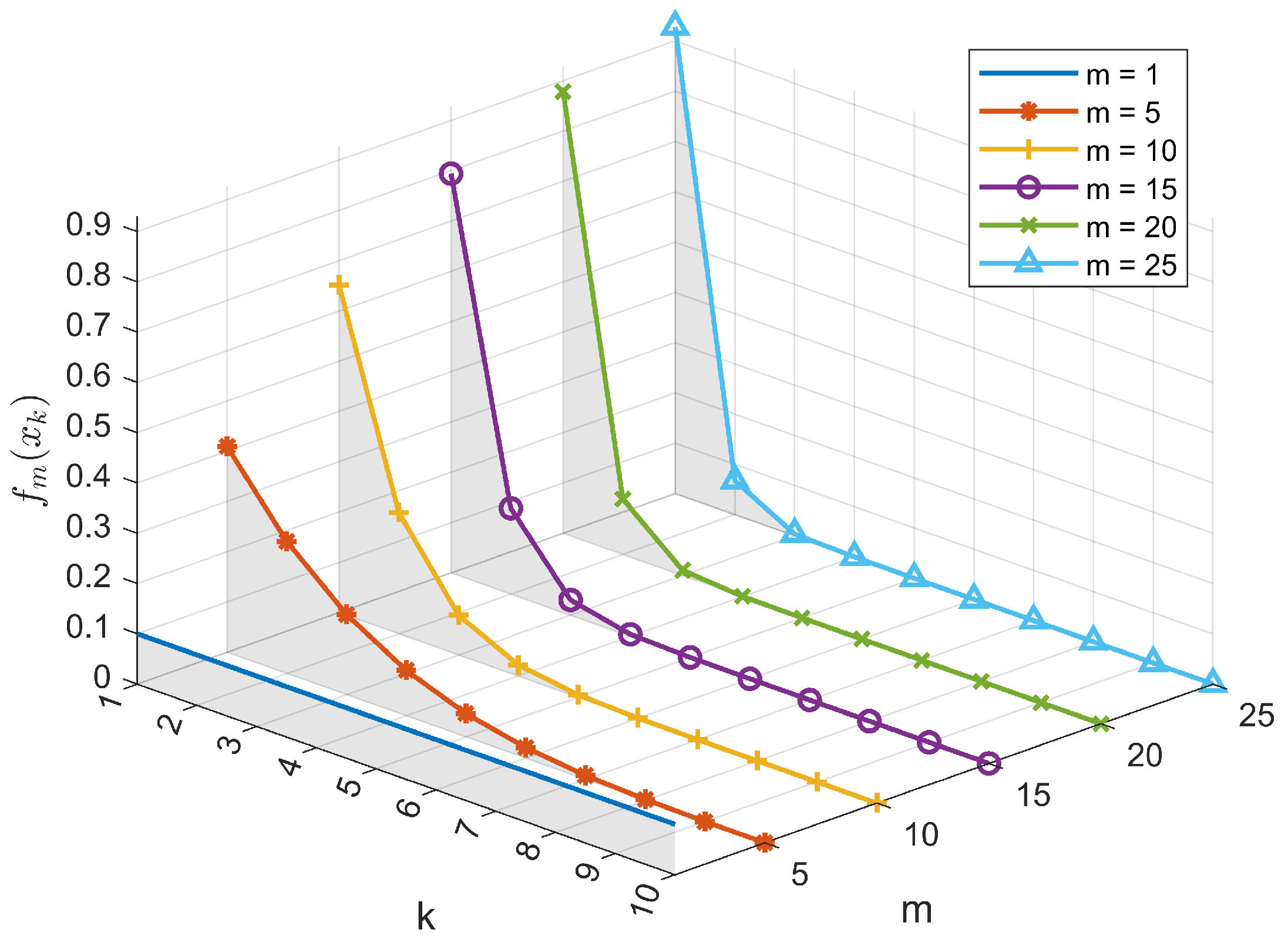
Next, we verify the bias of the probability distribution. For $1\le k\le n$, we first plot the following functions for different $m=1\mathrm{to}25$; see Figure 2.

$$f_{\wedge m}\left(x_k\right)={\left({\displaystyle \frac{n-k+1}{n}}\right)}^m-{\left({\displaystyle \frac{n-k}{n}}\right)}^m.$$

(48)

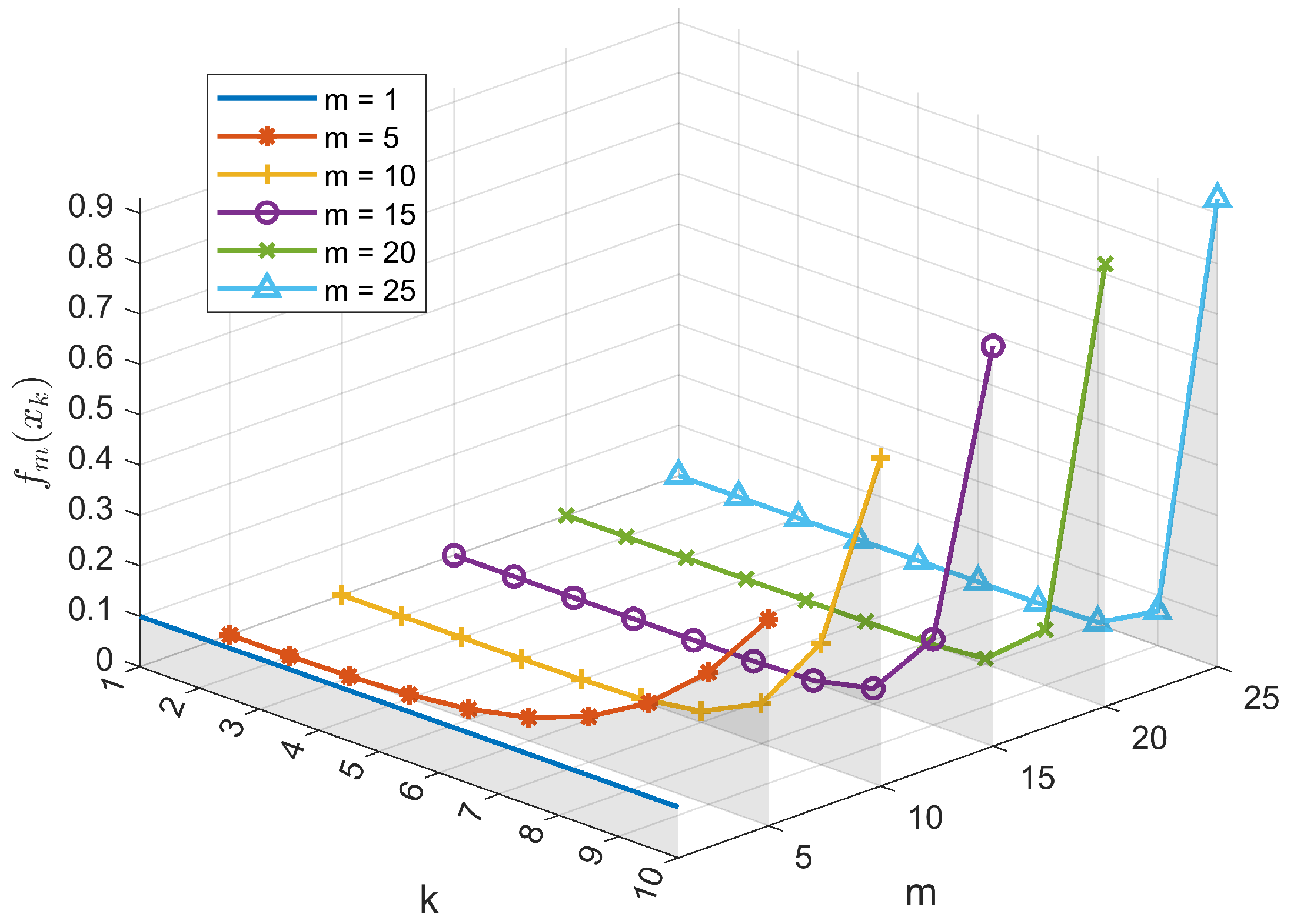
We can observe that when $m=1$, $R_f^{\wedge m}=R_f$ follows an (discrete) uniform distribution. As m increases, the probability distribution of $R_f^{\wedge m}$ becomes biased towards smaller values. This is an expected result, as the “$\wedge m$” operator increases the probability of smaller values occurring in $R_f$ while decreasing the probability of larger values. Note that the area of the shaded part is always 1. For $R_f^{\vee m}$, there is a symmetric result; see Figure 3.

Next, we present the graph of function $f_m\left(x_k\right)={\left[{\sum }_{i=k}^{n}f\left(x_i\right)\right]}^m-{\left[{\sum }_{i=k+1}^{n}f\left(x_i\right)\right]}^m$ when $f\left(x\right)={\displaystyle \frac{1}{n}}$. If $m=1$, function $f_m\left(x_k\right)$ is uniformly distributed. As m increases, function $f_m\left(x_k\right)$ has a significant biasing effect on the distribution of $f\left(x\right)$, See Figure 4.

Therefore, $R_f^m$ and $R_f^{\vee m}$ have similar effects on $R_f$. Both will bias the distribution of $R_f$ toward larger values, although to different extents.

Thus, we can obtain the probability distribution of superposed transitive closures of a classical probability superposed fuzzy matrix.

Theorem 8. 

For an $N\times N$ classical probability fuzzy matrix ${\mathbf{R}}_f={\left[R_f\right]}_{N\times N}$ with $R_f={⨁}_{k=1}^n{\displaystyle \frac{1}{n}}|x_k\rangle$, its transitive closure ${\mathbf{R}}_f^{+}={\left[R_f^{+}\right]}_{N\times N}$ can be computed by the following equation:

$$R_f^{+}\approx \underset{k=1}{\overset{n}{⨁}}\left[{\left(1-{(1-{\displaystyle \frac{k}{n}})}^N\right)}^{N^{N-1}}-{\left(1-{(1-{\displaystyle \frac{k-1}{n}})}^N\right)}^{N^{N-1}}\right]|x_k\rangle$$

(49)

when N is sufficiently large.

We perform simulation verification of “approximately equal” in Equation (49). Let

$$f_{+}\left(x_k\right)={\left(1-{(1-{\displaystyle \frac{k}{n}})}^N\right)}^{N^{N-1}}-{\left(1-{(1-{\displaystyle \frac{k-1}{n}})}^N\right)}^{N^{N-1}}.$$

(50)

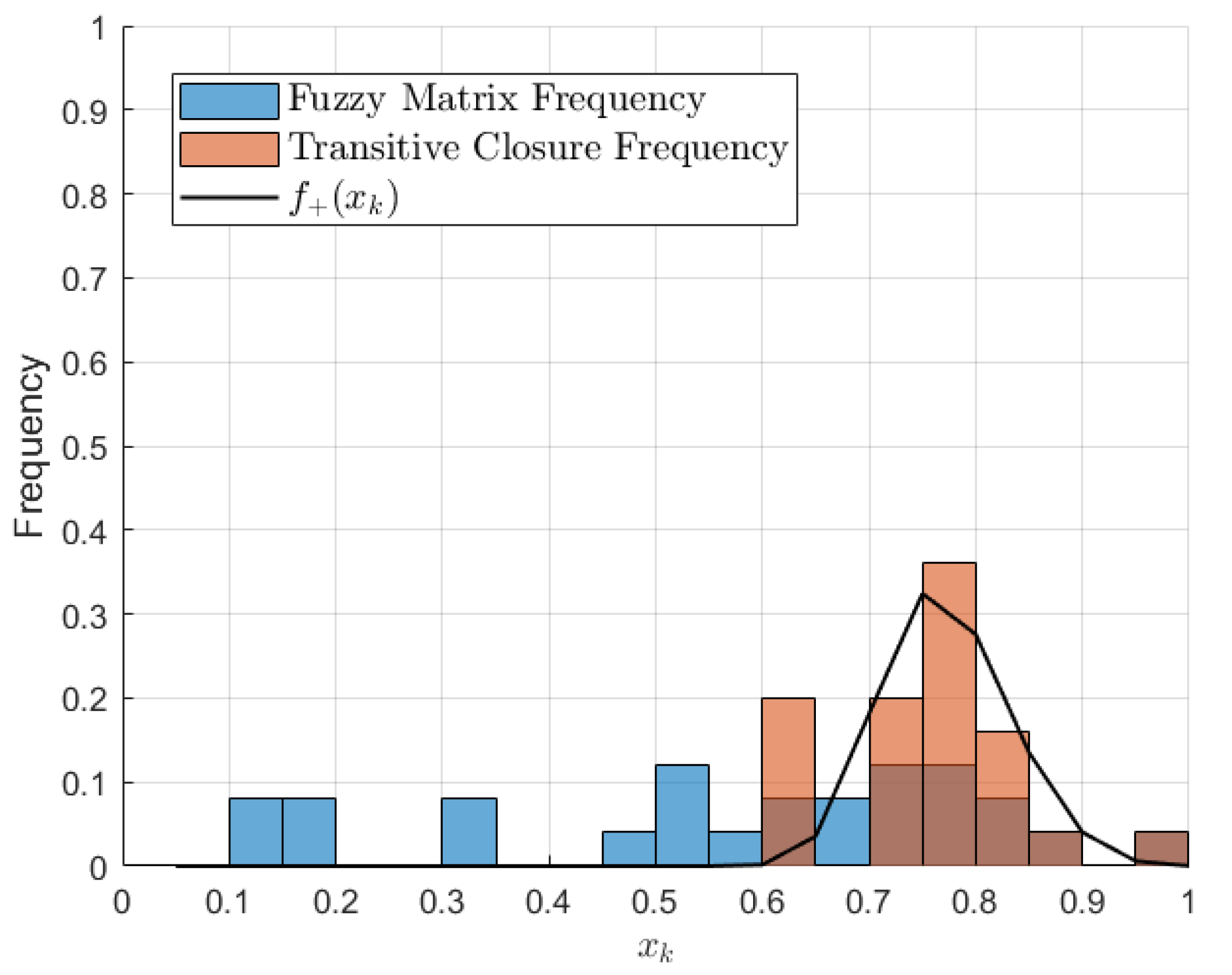
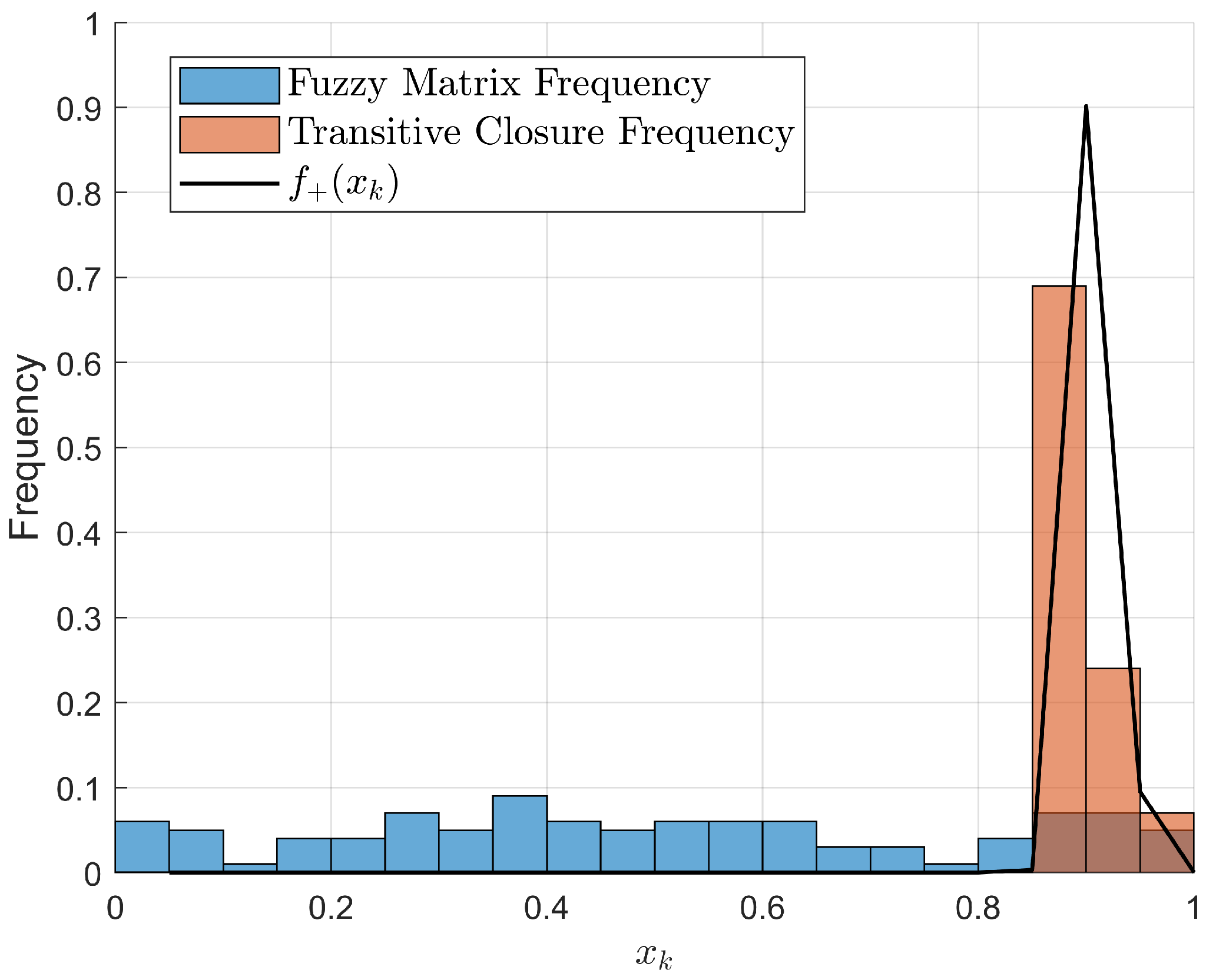
We plotted the function $f_{+}\left(x_k\right)$ for $N=5$, $n=20$ and $N=10$, $n=20$; see Figure 5 and Figure 6. Then, we constructed a fuzzy matrix using a uniform distribution and recorded the frequency of each element in that matrix. Next, we computed its transitive closure and recorded the frequency of each element in the transitive closure. It is important to note that N should not be too large, as this could exceed the computational capacity of the computer due to double exponentiation.

We found that the function $f_{+}\left(x_k\right)$ closely fits the probability/frequency distribution of the elements in the transitive closure. This also confirms that this approximate computation method for the transitive closure is feasible.

At the same time, we also obtain the probability distribution of superposed transitive closure of the classical probability superposed fuzzy matrix.

Proposition 6. 

Let $X=x_1,x_2,\dots ,x_n$ ($x_1\le x_2\le \cdots x_n$) be a random variable following uniform distribution. For a classical probability superposed fuzzy matrix ${\mathbf{R}}_f={\left[R_f\right]}_{N\times N}$, where $R_f={⨁}_{k=1}^n{\displaystyle \frac{1}{n}}|x_k\rangle$, the expectation of its transitive closure $R_f^{+}$ is

$$\mathbf{Exp}\left[R_f^{+}\right]\approx max\{x\mid x\in X\}-\sum _{k=1}^{n-1}{\left[1-{\left(1-{\displaystyle \frac{k}{n}}\right)}^N\right]}^{N^{N-1}}(x_{k+1}-x_k).$$

(51)

4. Conclusions

This study introduces the concept of randomly generated fuzzy matrices and their transitive closures, expanding the theoretical framework of traditional fuzzy matrices to effectively address uncertainties commonly found in fuzzy systems. By incorporating the notion of superposition from quantum mechanics, this work presents “superposed fuzzy relations” to represent probabilistic fuzzy relationships among elements, offering a novel approach to modeling fuzzy relations under uncertain conditions. First, the study defines the “min” and “max” operations for superposed fuzzy relations and derives the probability distributions of transitive closures for finite-dimensional superposed fuzzy matrices. This approach extends traditional operations on fuzzy relations, making fuzzy modeling more expressive in uncertain environments. The important point is that this paper presents an explicit functional relationship between two types of superimposed fuzzy matrices and their transitive closures. This functional relationship enables us to directly calculate the expected value of the transitive closure by using the probability distribution of the original matrix.

There is still much work to be done in the future. The study in this paper focuses on the superposed fuzzy relation, which is independent of the elements, meaning that all elements in the fuzzy matrix are generated from a single probability distribution. We need to continue exploring the transitive closure of superposed fuzzy relations that are dependent on the elements. In addition, the transitive closure of the fuzzy matrix for the superposition of any discrete random variables needs to be studied.

References

1. Zadeh, L.A. Fuzzy sets. Inf. Control 1965, 8, 338–353. [Google Scholar] [CrossRef]
2. Naessens, H.; De Meyer, H.; De Baets, B. Algorithms for the computation of T-transitive closures. IEEE Trans. Fuzzy Syst. 2002, 10, 541–551. [Google Scholar] [CrossRef]
3. Lee, H.S. An optimal algorithm for computing the max–min transitive closure of a fuzzy similarity matrix. Fuzzy Sets Syst. 2001, 123, 129–136. [Google Scholar] [CrossRef]
4. Baier, C.; Katoen, J.P. Principles of Model Checking; MIT Press: Cambridge, MA, USA, 2008. [Google Scholar]
5. Ma, Z.; Li, Z.; Li, W.; Gao, Y.; Li, X. Model checking fuzzy computation tree logic based on fuzzy decision processes with cost. Entropy 2022, 24, 1183. [Google Scholar] [CrossRef] [PubMed]
6. Dubois, D.; Prade, H. Fuzzy set and possibility theory-based methods in artificial intelligence. Artif. Intell. 2003, 148, 1–9. [Google Scholar] [CrossRef]
7. Ying, H.; Lin, F. Self-learning fuzzy automaton with input and output fuzzy sets for system modelling. IEEE Trans. Emerg. Top. Comput. Intell. 2022, 7, 500–512. [Google Scholar] [CrossRef]
8. Liu, W.; He, Q.; Li, Z.; Li, Y. Self-learning modeling in possibilistic model checking. IEEE Trans. Emerg. Top. Comput. Intell. 2024, 8, 264–278. [Google Scholar] [CrossRef]
9. Liu, W.; Wang, J.; He, Q.; Li, Y. Model checking computation tree logic over multi-valued decision processes and its reduction techniques. Chin. J. Electron. 2024, 33, 1399–1411. [Google Scholar] [CrossRef]
10. Sakurai, J.J.; Napolitano, J. Modern Quantum Mechanics; Cambridge University Press: Cambridge, UK, 2020. [Google Scholar]
11. Liu, W.; Li, Z.; Li, Y. Quantum Reachability Games. IEEE Trans. Emerg. Top. Comput. Intell. 2024, 1–15. Available online: https://ieeexplore.ieee.org/document/10584096 (accessed on 3 July 2024). [CrossRef]
12. Kruse, R.; Buck-Emden, R.; Cordes, R. Processor power considerations—An application of fuzzy Markov chains. Fuzzy Sets Syst. 1987, 21, 289–299. [Google Scholar] [CrossRef]
13. Buckley, J.J. Fuzzy probabilities: New approach and applications. Physica 2012, 115, 7–30. [Google Scholar]
14. Kurano, M.; Yasuda, M.; Nakagami, J.i.; Yoshida, Y. A fuzzy approach to Markov decision processes with uncertain transition probabilities. Fuzzy Sets Syst. 2006, 157, 2674–2682. [Google Scholar] [CrossRef]
15. Zadeh, L.A. Fuzzy probabilities. Inf. Process. Manag. 1984, 20, 363–372. [Google Scholar] [CrossRef]
Figure 1. Proportion of 0.8 and 0.2 elements in transitive closure with different sizes of fuzzy matrix.
Axioms 14 00690 g001
Figure 2. The distribution bias of classical probability superposed fuzzy relation R f m .
Axioms 14 00690 g002
Figure 3. The distribution bias of classical probability superposed fuzzy relation R f m .
Axioms 14 00690 g003
Figure 4. The bias of R f = k = 1 n 1 n | x k under the role of m-th power operator.
Axioms 14 00690 g004
Figure 5. Element frequency of fuzzy matrix and its transitive closure, and f + ( x k ) with N = 5 , n = 20 .
Axioms 14 00690 g005
Figure 6. Element frequency of fuzzy matrix and its transitive closure, and f + ( x k ) with N = 10 , n = 20 .
Axioms 14 00690 g006
Disclaimer/Publisher’s Note: The statements, opinions and data contained in all publications are solely those of the individual author(s) and contributor(s) and not of MDPI and/or the editor(s). MDPI and/or the editor(s) disclaim responsibility for any injury to people or property resulting from any ideas, methods, instructions or products referred to in the content.