Article

Existence and Uniqueness of Solutions for Impulsive Stochastic Differential Variational Inequalities with Applications

School of Mathematical and Statistics, Guizhou University, Guiyang 550025, China
*
Author to whom correspondence should be addressed.
Axioms 2025, 14(8), 603; https://doi.org/10.3390/axioms14080603 (registering DOI)
Submission received: 17 June 2025 / Revised: 19 July 2025 / Accepted: 29 July 2025 / Published: 3 August 2025

Abstract

This paper focuses on exploring an impulsive stochastic differential variational inequality (ISDVI), which combines an impulsive stochastic differential equation and a stochastic variational inequality. Innovatively, our work incorporates two key aspects: first, our stochastic differential equation contains an impulsive term, enabling better handling of sudden event impacts; second, we utilize a non-local condition z ( 0 ) = χ 0 + ϑ ( z ) that integrates measurements from multiple locations to construct superior models. Methodologically, we commence our analysis by using the projection method, which ensures the existence and uniqueness of the solution to ISDVI. Subsequently, we showcase the practical applicability of our theoretical findings by implementing them in the investigation of a stochastic consumption process and electrical circuit model.

1. Introduction

Variational inequality theory has been widely applied in economics, management science, cybernetics, and transportation. It has become a fundamental pillar of nonlinear analysis [1,2,3]. Differential variational inequalities (DVIs) are coupled with differential equations and variational inequalities. DVIs initially appeared in the research of Aubin and Cellina [4] in 1984. Subsequently, Pang and Stewart [5] emerged as trailblazers, meticulously presenting and delving into DVIs within finite-dimensional Euclidean spaces. In doing so, they artfully laid the theoretical cornerstone for this field of study. DVIs are widely used in circuit systems, economic dynamics, and traffic networks, among others. To date, numerous scholars have investigated DVIs under various conditions and achieved significant progress, as shown in [6,7,8,9,10]. Notable contributions include, for example, the study in [11], where the authors introduced an inverse variational inequality. In [12,13,14,15,16,17,18], the authors further explored fractional differential and hemivariational inequalities in depth.
Impulsive differential systems have emerged as a prominent research domain in modeling real-world processes characterized by abrupt changes at discrete time points. These systems, originating from the need to describe instantaneous perturbations, have expanded into various applications in mechatronics, telecommunications, neural networks, and financial economics, as documented in seminal works [19,20,21,22,23,24,25,26].
Importantly, stochastic differential variational inequalities (SDVIs), which integrate stochastic differential equations and variational inequalities, have garnered significant research attention owing to their unique advantages and extensive application potential [27]. In fields such as economic analysis, traffic equilibrium, and energy modeling, SDVIs have emerged as a powerful tool for handling complex stochastic phenomena and inequality-constrained problems. Given the increasing need to model differential equations and variational inequalities in applied sciences, deepening research on SDVIs involving stochastic differential constraints becomes particularly imperative. For a more comprehensive understanding, one can refer to the literature on stochastic planning [28,29,30,31].
Drawing from the literature, this paper explores an impulsive stochastic differential variational inequality (ISDVI), as defined below:
d z ( s ) = b 1 ( s , z ( s ) , v ( s ) ) d s + b 2 ( s , z ( s ) , v ( s ) ) d W ( s ) , s δ , s s j , Δ z ( s j ) = I j ( z ( s j ) ) , j = 1 , 2 , , m , z ( 0 ) = χ 0 + ϑ ( z ) , G ( s , ω , z ( s ) , v ( s ) ) , u v ( s ) 0 , u U , a . e . s δ , a . s . ω Ω .
Let δ = [ 0 , T ] , and consider the continuous functions G : δ × Ω × R n × U R m , b 1 : δ × R n × R m R n , and b 2 : δ × R n × R m R n × h . The processes z ( s ) = z ( s , ω ) and v ( s ) = v ( s , ω ) represent the state and control variables, respectively. Here, χ s (with χ 0 denoting the initial-history component of the system, i.e., the specific value of this history function at the initial time s = 0 ) represents a history function that satisfies E χ 0 2 < and that ϑ ( z ) is a continuous functional. W ( s ) denotes a standard h-dimensional Brownian motion. I j : R n R n is an impulsive function with j = 1 , 2 , , m , Δ z ( s j ) is given by Δ z ( s j ) = z ( s j + ) z ( s j ) with z ( s j + ) and z ( s j ) being the right and left limit of z at s = s j , respectively, and 0 = s 0 < s 1 < < s m < s m + 1 = T . The set of controls U is a convex and closed subset within R m .
Here are several specific examples of (1).
(i)
If ϑ ( z ) = 0 in (1), then it transforms into the following problem: find z : δ × Ω H [ 0 , T ] and v : δ × Ω V [ 0 , T ] , such that
d z ( s ) = b 1 ( s , z ( s ) , v ( s ) ) d s + b 2 ( s , z ( s ) , v ( s ) ) d W ( s ) , s δ , s s j , Δ z ( s j ) = I j ( z ( s j ) ) , j = 1 , 2 , , m , z ( 0 ) = χ 0 , G ( s , ω , z ( s ) , v ( s ) ) , u v ( s ) 0 , u U , a . e . s δ , a . s . ω Ω ,
which is still a new problem.
(ii)
If I j = 0 , ϑ ( z ) = 0 in (1), then it simplifies to the subsequent problem: find z : δ × Ω H [ 0 , T ] and v : δ × Ω V [ 0 , T ] , such that
d z ( s ) = b 1 ( s , z ( s ) , v ( s ) ) d s + b 2 ( s , z ( s ) , v ( s ) ) d W ( s ) , s δ , z ( 0 ) = χ 0 , G ( s , ω , z ( s ) , v ( s ) ) , u v ( s ) 0 , u U , a . e . s δ , a . s . ω Ω ,
which was discussed by Zhang et al. in [32].
Impulsive stochastic differential equations are not widely applied at present. Our present research explores this direction. This paper innovates in the following three aspects: (i) Different from the work in [32,33,34], our stochastic differential equation contains an impulsive term. Mathematically, dealing with the impulsive term brings us certain difficulties: e.g., the impulsive term will make the state trajectory of the system discontinuous, requiring the behavior of the solution to be considered in separate time intervals, which complicates the establishment of continuity and differentiability conditions. But it can better handle the impacts of sudden events. (ii) Different from the work in [35], we use the non-local condition z ( 0 ) = χ 0 + ϑ ( z ) , which incorporates measurements from multiple locations to construct superior models. (iii) We apply impulsive stochastic differential equations to the consumption process and electrical circuit model in a stochastic environment and demonstrate the practical applications of these findings.
The layout of this paper is structured as below. In Section 2, fundamental definitions and initial results are presented. Section 3 focuses on examining the existence of mild solutions to (1). In Section 4, we present two case studies to confirm our theoretical conclusions, and Section 5 wraps up with concluding remarks.

2. Preliminaries

In this part, we introduce the essential concepts that form the foundation for the following sections.
We suppose ( Ω , F , P , { F s } s 0 ) constitutes a complete probability space, with { F s } s 0 serving as the filtration. · and · , · represent the norm and inner product of R n (or R m ), respectively, and the norm of R n × h is denoted by · n × h . The measurable space L 2 ( Ω , R n ) , which is equivalent to L 2 ( Ω , P , F , R n ) , is constituted by all square integrable random variables. This space L 2 ( Ω , R n ) can be treated as a Hilbert space, and it is equipped with the norm · L 2 = E · 2 1 2 .
The Hilbert space of all stochastic processes g ( s , ω ) is denoted by H [ c , d ] = L 2 ( [ c , d ] × Ω , R n ) . Here, the processes g ( s , ω ) have values in R n , and the parameters satisfy 0 c d T < . These processes not only satisfy the condition c d E g ( s , ω ) 2 d t < , but are also adapted to the filtration { F s } . For any z H [ c , d ] , its norm is defined as z H [ c , d ] = c d E z ( s , ω ) 2 d s 1 2 . Moreover, for any u , v H [ c , d ] , the inner product is given by u , v H [ c , d ] = c d E [ u ( s , ω ) , v ( s , ω ) ] d s .
Suppose U is a non-empty subset of R m . For any given interval [ c , d ] that is a subset of δ , we define
V [ c , d ] = { v L 2 ( [ c , d ] × Ω , R m ) : v ( s ) U , a . e . s [ c , d ] , a . s . ω Ω . } ,
where V [ c , d ] represents the set of admissible control functions over the time interval [ c , d ] .
Lemma 1
([34] (p. 3)). Given that U R m is convex, closed, and nonempty, for every interval [ c , d ] δ , the set V [ c , d ] remains nonempty, closed, and convex within L 2 ( [ c , d ] × Ω , R m ) .
Lemma 2
([33] (p. 3)). Let H be a Hilbert space and U be a non-empty, closed, convex subset of H. For any u H , the projection of u onto U, denoted as v = P U ( u ) , is defined as mapping that projects u to the nearest point in U. Suppose v 1 = P U ( u 1 ) and v 2 = P U ( u 2 ) for any u 1 , u 2 H . Subsequently, the following inequality is satisfied:
v 1 v 2 2 u 1 u 2 2 .
Lemma 3
([32] (p. 3)). Let H be a Hilbert space and U be a non-empty, closed, convex subset of H. Take an operator Y : H H . The following inequality
Y ( v ) , z v 0 , z U ,
has a solution v U , where v = P U ( ( J c Y ) ( v ) ) , with c > 0 and J denoting the identity operator.
Lemma 4
([34] (p. 3)). Suppose v V [ c , d ] . Then, for every fixed z H [ c , d ] , this inequality
G ( s , ω , z ( s ) , v ( s ) ) , u v ( s ) 0 , u U , a . e . s [ c , d ] , a . s . ω Ω ,
corresponds to the inequality
G ˜ ( z , v ) , u 1 v H [ c , d ] 0 , u 1 V [ c , d ] .
Here, the function G ˜ : H [ c , d ] × V [ c , d ] L 2 ( [ c , d ] × Ω , R m ) is defined as
G ˜ ( z , v ) : = G ( t , ω , z ( s ) , v ( s ) ) ,
( z , v ) H [ c , d ] × V [ c , d ] , ω Ω , s [ c , d ] .
Lemma 5
([33] (p. 4)). For every N > 0 , the space L 2 ( 0 , N ) consists of functions satisfying measurability, adaptedness, and square integrability. For any such function g L 2 ( 0 , N ) , the Itô isometry states that
E 0 T g ( θ ) d W ( θ ) 2 = E 0 T g 2 ( θ ) d θ , g L 2 ( 0 , N ) .
Problem 1.
Find a pair ( z ( s ) , v ( s ) ) H [ 0 , T ] × V [ 0 , T ] , such that
d z ( s ) = b 1 ( s , z ( s ) , v ( s ) ) d s + b 2 ( s , z ( s ) , v ( s ) ) d W ( s ) , s δ , s s j , Δ z ( s j ) = I j ( z ( s j ) ) , j = 1 , 2 , , m , z ( 0 ) = χ 0 + ϑ ( z ) , v ( s ) SOL ( V [ 0 , T ] , G ( s , ω , z ( s ) , v ( s ) ) ) .
The notation SOL ( V [ 0 , T ] , G ( s , ω , z ( s ) , v ( s ) ) ) denotes the solution set of the variational inequality that seeks to find v V [ 0 , T ] , such that
G ( s , ω , z ( s ) , v ( s ) ) , u v ( s ) 0 , u U , a . e . s δ , a . s . ω Ω .
When studying Problem 1, we consider the subsequent impulsive Cauchy problem:
d z ( s ) = φ 1 ( s ) d s + φ 2 ( s ) d W ( s ) , s δ , s s j , Δ z ( s j ) = I j ( z ( s j ) ) , j = 1 , 2 , , m , z ( 0 ) = χ 0 + ϑ ( z ) .
Lemma 6.
The Cauchy problem
d z ( s ) = φ 1 ( s ) d s + φ 2 ( s ) d W ( s ) , s δ , s s j , Δ z ( s j ) = I j ( z ( s j ) ) , j = 1 , 2 , , m , z ( 0 ) = χ 0 + ϑ ( z ) ,
holds an equivalence relation with the integral equation
z ( s ) = χ 0 + ϑ ( z ) + 0 s φ 1 ( θ ) d θ + 0 s φ 2 ( θ ) d W ( θ ) + i = 1 j I i ( z ( s i ) ) .
Proof. 
Assume that (4) holds. If s [ 0 , s 1 ] , one has
d z ( s ) = φ 1 ( s ) d s + φ 2 ( s ) d W ( s ) , s [ 0 , s 1 ] with z ( 0 ) = χ 0 + ϑ ( z ) .
Integrating (6) from 0 to s 1 , then
z ( s ) = χ 0 + ϑ ( z ) + 0 s φ 1 ( θ ) d θ + 0 s φ 2 ( θ ) d W ( θ ) .
If s ( s 1 , s 2 ] , one has
d z ( s ) = φ 1 ( s ) d s + φ 2 ( s ) d W ( s ) , s ( s 1 , s 2 ] with z ( s 1 + ) = z ( s 1 ) + I 1 ( z ( s 1 ) ) ,
then
z ( s ) = z ( s 1 + ) + 0 s φ 1 ( θ ) d θ + 0 s φ 2 ( θ ) d W ( θ ) = z ( s 1 ) + I 1 ( z ( s 1 ) ) + 0 s φ 1 ( θ ) d θ + 0 s φ 2 ( θ ) d W ( θ ) = χ 0 + ϑ ( z ) + I 1 ( z ( s 1 ) ) + 0 s φ 1 ( θ ) d θ + 0 s φ 2 ( θ ) d W ( θ ) .
If s ( s 2 , s 3 ] , one has
z ( s ) = z ( s 2 + ) + 0 s φ 1 ( θ ) d θ + 0 s φ 2 ( θ ) d W ( θ ) = z ( s 2 ) + I 2 ( z ( s 2 ) ) + 0 s φ 1 ( θ ) d θ + 0 s φ 2 ( θ ) d W ( θ ) = χ 0 + ϑ ( z ) + I 1 ( z ( s 1 ) ) + I 2 ( z ( s 2 ) ) + 0 s φ 1 ( θ ) d θ + 0 s φ 2 ( θ ) d W ( θ ) .
Similarly, if s ( s j , s j + 1 ] , we can show that
z ( s ) = χ 0 + ϑ ( z ) + 0 s φ 1 ( θ ) d θ + 0 s φ 2 ( θ ) d W ( θ ) + i = 1 j I i ( z ( s i ) ) .
Conversely, assume that (5) is valid. When s ( 0 , s 1 ] , we are aware that (4) holds. For s ( s j , s j + 1 ] , where j = 1 , 2 , , m , because the derivative of a constant is zero, we have d z ( s ) = φ 1 ( s ) d s + φ 2 ( s ) d W ( s ) for s ( s j , s j + 1 ] , and Δ z ( s j ) = I j ( z ( s j ) ) . □
Definition 1.
A pair ( z ( s ) , v ( s ) ) is called a mild solution of Problem 1 if and only if
z ( s ) = χ 0 + ϑ ( z ) + 0 s b 1 ( θ , z ( θ ) , v ( θ ) ) d θ + 0 s σ ( θ , z ( θ ) , v ( θ ) ) d W ( θ ) + i = 1 j I i ( z ( s i ) ) , v ( t ) SOL ( U [ 0 , T ] , G ( s , ω , z ( s ) , v ( s ) ) ) ,
where s ( s j , s j + 1 ] , j = 1 , 2 , , m .

3. Existence and Uniqueness of ISDVI

Hypothesis 1.
Consider elements z , z 1 , z 2 R n , v , v 1 , v 2 R m , a parameter t δ , functions z , z 1 , z 2 H [ 0 , T ] , and v 1 , v 2 V [ 0 , T ] . Let K b 1 , K b 2 , L b 1 , L b 2 , L I i , L ϑ , L G , M , C be positive constants, such that L G > M . The following properties hold:
H( b 1 )
The function b 1 : δ × R n × R m R n satisfies the following conditions:
(i) 
Boundedness: b 1 ( s , z , v ) 2 K b 1 ( 1 + z 2 + v 2 ) .
(ii) 
Lipschitz continuity: b 1 ( s , z 1 , v 1 ) b 1 ( s , z 2 , v 2 ) 2 L b 1 ( z 1 z 2 2 + v 1 v 2 2 ) .
H( b 2 )
The function b 2 : δ × R n × R m R n × h adheres to the subsequent conditions:
(i) 
Boundedness: b 2 ( s , z , v ) R n × h 2 K b 2 ( 1 + z 2 + v 2 ) .
(ii) 
Lipschitz continuity: b 2 ( s , z 1 , v 1 ) b 2 ( s , z 2 , v 2 ) R n × h 2 L b 2 ( z 1 z 2 2 + v 1 v 2 2 ) .
H( G ˜ )
The function G : δ × Ω × R n × U R m meets the ensuing requirements:
(i) 
G ˜ ( z 1 , v 1 ) G ˜ ( z 2 , v 2 ) L G ( z 1 z 2 + v 1 v 2 ) .
(ii) 
G ˜ ( z , v 1 ) G ˜ ( z , v 2 ) , v 1 v 2 M v 1 v 2 2 .
H( I i )
The function I i : R n R n meets the subsequent criteria:
(i) 
For each index i = 1 , 2 , 3 , , m , there exists a constant d i , such that for every z H [ 0 , T ] , we have I i ( z ) d i .
(ii) 
Lipschitz continuity: I i ( z 1 ) I i ( z 2 ) L I i z 1 z 2 .
H( ϑ )
The function ϑ: R n R n satisfies the following conditions:
(i) 
Growth condition: ϑ ( z ) 2 C z 2 .
(ii) 
Lipschitz continuity: ϑ ( z 1 ) ϑ ( z 2 ) 2 L ϑ z 1 z 2 2 .
Additionally, the following lemmas are required.
Lemma 7.
Provided that the function G ˜ meets the requirements in H ( G ˜ ) of Hypothesis 1, the subsequent assertion is valid: For any fixed z H [ 0 , c ] ( 0 < c T ) , there exists a unique v V [ 0 , c ] , satisfying:
G ( s , ω , z ( s ) , v ( s ) ) , u v ( s ) 0 , u U , a . e . s [ 0 , c ] , a . s . ω Ω .
Proof. 
By defining v q + 1 ( s ) = P V [ 0 , c ] [ v q ( s ) ρ G ˜ ( z ( s ) , v q ( s ) ) ] . To establish the uniqueness of v, we aim to show that the mapping T ( v ) = P V [ 0 , c ] v ρ G ˜ ( z , v ) is a contraction mapping on V [ 0 , c ] .
Leveraging condition H ( G ˜ ) in Hypothesis 1, along with Lemma 2, we find that
v q + 1 ( s ) v q ( s ) H [ 0 , c ] 2 = P V [ 0 , c ] [ v q ( s ) ρ G ˜ ( z ( s ) , v q ( s ) ) ] P V [ 0 , c ] [ v q 1 ( s ) ρ G ˜ ( z ( s ) , v q 1 ( s ) ) ] H [ 0 , c ] 2 v q ( s ) v q 1 ( s ) ρ G ˜ ( z ( s ) , v q ( s ) ) + ρ G ˜ ( z ( s ) , v q 1 ( s ) ) H [ 0 , c ] 2 = v q ( s ) v q 1 ( s ) H [ 0 , c ] 2 + ρ 2 G ˜ ( z ( s ) , v q 1 ( s ) ) G ˜ ( z ( s ) , v q ( s ) ) H [ 0 , c ] 2 2 ρ G ˜ ( z ( s ) , v q ( s ) ) G ˜ ( z ( s ) , v q 1 ( s ) ) , v q ( s ) v q 1 ( s ) H [ 0 , c ] ( 1 2 ρ M + ρ 2 L G 2 ) v q ( s ) v q 1 ( s ) H [ 0 , c ] 2 ,
where 0 < ρ < 2 M L G 2 , ensuring that { v n } forms a Cauchy sequence in V [ 0 , c ] . As a result, a unique v * exists such that v ( n ) v * . Furthermore, the dominated convergence theorem combined with the continuity of P V [ 0 , c ] produces the following conclusion:
v * = lim n P V [ 0 , c ] ( v ( n ) ( s ) ρ G ˜ ( z ( n ) , v ( n ) ) = P V [ 0 , c ] ( v * ρ G ˜ ( z * , v * ) ) .
This implies v * = T ( v * ) , so v * is a fixed point of T . According to the Banach fixed-point theorem, this fixed point is unique.
Using Lemmas 1 and 3, we have
G ˜ ( z , v * ) , u 2 v * H [ 0 , c ] 0 , u 2 V [ 0 , c ] .
From Lemma 4, we obtain that v q ( s ) = P V [ 0 , c ] ( v q ( s ) ρ G ˜ ( z q ( s ) , v q ( s ) ) ) , where
G ( s , ω , z ( s ) , v ( s ) ) , u v ( s ) 0 , u U , a . e . s [ 0 , c ] , a . s . ω Ω ,
if v q 1 V [ 0 , c ] , then v q V [ 0 , c ] as well. □
Lemma 8
([32] (p. 4)). Provided that the function G ˜ meets the requirements in H ( G ˜ ) of Hypothesis 1, the subsequent assertion is valid: For each i = 1 , 2 , given any fixed z i H [ 0 , T ] , a unique v i V [ 0 , T ] exists, fulfilling the subsequent condition:
G ( s , ω , z i ( s ) , v i ( s ) ) , u v i ( s ) 0 , u U , a . e . s δ , a . s . ω Ω .
Additionally, a positive constant D exists, with the following inequality holding:
E 0 s v 1 ( θ , ω ) v 2 ( θ , ω ) 2 d θ D E 0 s z 1 ( θ , ω ) z 2 ( θ , ω ) 2 d θ .
Lemma 9.
Under Hypothesis 1, the following holds: For any fixed v V [ 0 , c ] ( 0 < c T ) , there exists a unique z H [ 0 , c ] satisfying the following condition:
d z ( s ) = b 1 ( s , z ( s ) , v ( s ) ) d s + b 2 ( s , z ( s ) , v ( s ) ) d W ( s ) , s [ 0 , c ] , s s j , Δ z ( s j ) = I j ( z ( s j ) ) , j = 1 , 2 , , m , z ( 0 ) = χ 0 + ϑ ( z ) .
Proof. 
Define operator Σ : H [ 0 , c ] H [ 0 , c ] by setting
( Σ z ) ( s ) = χ 0 + ϑ ( z ) + 0 s b 1 ( θ , z ( θ ) , v ( θ ) ) d θ + 0 s b 2 ( θ , z ( θ ) , v ( θ ) ) d W ( θ ) + i = 1 j I i ( z ( s i ) ) ,
which is well defined. To prove Lemma 9, it suffices to show that Σ has a unique fixed point in H [ 0 , c ] .
Subsequently, we prove that Σ is a contractive map. For z 1 , z 2 H [ 0 , c ] , using the Cauchy–Schwarz inequality, we obtain
E ( Σ z 1 ) ( s ) ( Σ z 2 ) ( s ) 2 4 E ϑ ( z 1 ) ϑ ( z 2 ) 2 + 4 E 0 s [ b 1 ( θ , z 1 ( θ ) , v ( θ ) ) b 1 ( θ , z 2 ( θ ) , v ( θ ) ) ] d θ 2 + 4 E 0 s [ b 2 ( θ , z 1 ( θ ) , v ( θ ) ) b 2 ( θ , z 2 ( θ ) , v ( θ ) ) ] d W ( θ ) 2 + 4 E i = 1 j [ I i ( z 1 ( s i ) ) I i ( z 2 ( s i ) ) ] 2 .
By condition H ( ϑ ) of Hypothesis 1,
E ϑ ( z 1 ) ϑ ( z 2 ) 2 L ϑ E z 1 z 2 2 .
Using condition H ( b 1 ) from Hypothesis 1,
E 0 s [ b 1 ( θ , z 1 ( θ ) , v ( θ ) ) b 1 ( θ , z 2 ( θ ) , v ( θ ) ) ] d θ 2 E 0 s b 1 ( θ , z 1 ( θ ) , v ( θ ) ) b 1 ( θ , z 2 ( θ ) , v ( θ ) ) d θ 2 E 0 s L b 1 ( z 1 ( θ ) z 2 ( θ ) 2 + v ( θ ) v ( θ ) 2 ) d θ 2 = L b 1 E 0 s z 1 ( θ ) z 2 ( θ ) d θ 2 s L b 1 0 s E z 1 ( θ ) z 2 ( θ ) 2 d θ .
By virtue of condition H ( b 2 ) in Hypothesis 1,
E 0 s [ b 2 ( θ , z 1 ( θ ) , v ( θ ) ) b 2 ( θ , z 2 ( θ ) , v ( θ ) ) ] d W ( θ ) 2 = E 0 s b 2 ( θ , z 1 ( θ ) , v ( θ ) ) b 2 ( θ , z 2 ( θ ) , v ( θ ) ) 2 d θ L b 2 E 0 s ( z 1 ( θ ) z 2 ( θ ) 2 + v ( θ ) v ( θ ) 2 ) d θ = L b 2 0 s E z 1 ( θ ) z 2 ( θ ) 2 d θ .
In accordance with condition H ( I i ) of Hypothesis 1,
E i = 1 j [ I i ( z 1 ( s i ) ) I i ( z 2 ( s i ) ) ] 2 j L I i 2 i = 1 j E z 1 ( s i ) z 2 ( s i ) 2 .
Here, we can acquire
E ( Σ z 1 ) ( s ) ( Σ z 2 ) ( s ) 2 = 4 L ϑ E z 1 z 2 2 + ( 4 s L b 1 + 4 L b 2 ) 0 s E z 1 ( θ ) z 2 ( θ ) 2 d θ + 4 j L I i 2 i = 1 j E z 1 ( s i ) z 2 ( s i ) 2 .
Thus, based on the norm’s definition, we obtain
( Σ z 1 ) ( s ) ( Σ z 2 ) ( s ) = 0 c E ( Σ z 1 ) ( s ) ( Σ z 2 ) ( s ) 2 d s 1 2 0 c ( 4 L ϑ E z 1 z 2 2 + ( 4 s L b 1 + 4 L b 2 ) 0 s E z 1 ( θ ) z 2 ( θ ) 2 d θ ) d s 1 2 + 0 c 4 j L I i 2 i = 1 j E z 1 ( s i ) z 2 ( s i ) 2 d s 1 2 .
Let α ( θ ) = E z 1 ( θ ) z 2 ( θ ) 2 , β 1 = 4 L ϑ , β 2 = 4 L b 1 , β 3 = 4 L b 2 , β 4 = 4 j L I i 2 , then
( Σ z 1 ) ( s ) ( Σ z 2 ) ( s ) 0 c β 1 + β 2 c 2 θ 2 2 + β 3 ( c θ ) α ( θ ) d θ + β 4 0 c i = 1 j E z 1 ( s i ) z 2 ( s i ) 2 d s 1 2 .
Then, utilize z 1 z 2 = 0 c E z 1 z 2 2 d θ 1 2 = 0 c α ( θ ) d θ 1 2 to perform scaling.
Since β 1 + β 2 c 2 θ 2 2 + β 3 ( c θ ) has a maximum value on the interval θ [ 0 , c ] . When θ = 0 , β 1 + β 2 c 2 θ 2 2 + β 3 ( c θ ) = β 1 + β 2 c 2 2 + β 3 c .
Then
( Σ z 1 ) ( Σ z 2 ) β 1 + β 2 c 2 2 + β 3 c 0 c α ( θ ) d θ + β 4 0 c i = 1 j E z 1 ( s i ) z 2 ( s i ) 2 d s 1 2 .
Also, since 0 c i = 1 j E z 1 ( s i ) z 2 ( s i ) 2 d s j 0 c E z 1 ( θ ) z 2 ( θ ) 2 d θ = j 0 c α ( θ ) d θ , we have
( Σ z 1 ) ( Σ z 2 ) β 1 + β 2 c 2 2 + β 3 c + β 4 j 0 c α ( θ ) d θ 1 2 β 1 + β 2 c 2 2 + β 3 c + β 4 j 1 2 z 1 z 2 β z 1 z 2 ,
where β = ( β 1 + β 2 c 2 2 + β 3 c + β 4 j ) 1 2 . Since 0 < c T , L ϑ , L b 1 , L b 2 , and L I i are all positive constants.
When c is small enough,
β = ( β 1 + β 2 c 2 2 + β 3 c + β 4 j ) 1 2 = 2 ( L ϑ + L b 1 c 2 2 + L b 2 c + j 2 L I i 2 ) 1 2 < 1 .
Now we know that Σ is a contractive map, according to the Banach fixed-point theorem, Σ has a unique solution z H [ 0 , c ] . □
Theorem 1.
Under Hypothesis 1, the Problem 1 admits a unique solution ( z ( s ) , v ( s ) ) H [ 0 , T ] × V [ 0 , T ] .
Proof. 
We consider a sequence { z k ( s ) , v k ( s ) } , constructed as follows
z 1 ( s ) = χ 0 + ϑ ( z 1 ) , v k ( s ) = P V [ 0 , T ] v k ( s ) ρ G ˜ ( z k ( s ) , v k ( s ) ) , z k + 1 ( s ) = χ 0 + ϑ ( z k ) + 0 s b 1 ( θ , z k ( θ ) , v k ( θ ) ) d θ + 0 s b 2 ( θ , z k ( θ ) , v k ( θ ) ) d W ( θ ) + i = 1 j I i ( z k ( s i ) ) .
First, we show that ( z ( k + 1 ) ( s ) , v ( k + 1 ) ( s ) ) H [ 0 , T ] × V [ 0 , T ] by induction. For k = 1 , we have z 1 ( s ) = χ 0 + ϑ ( z 1 ) , by Lemma 7, there exists a unique v 1 ( s ) V [ 0 , T ] , satisfying v 1 ( s ) = P V [ 0 , T ] [ v 1 ( s ) ρ G ˜ ( z 1 ( s ) , v 1 ( s ) ) ] .
Let z 2 ( s ) = χ 0 + ϑ ( z 1 ) + 0 s b 1 ( θ , z 1 ( θ ) , v 1 ( θ ) ) d θ + 0 s b 2 ( θ , z 1 ( θ ) , v 1 ( θ ) ) d W ( θ ) + i = 1 j I i ( z ( s i ) ) H [ 0 , T ] . Again, by Lemma 7, there exists a unique v 2 ( s ) V [ 0 , T ] , satisfying v 2 ( s ) = P V [ 0 , T ] [ v 2 ( s ) ρ G ˜ ( z 2 ( s ) , v 2 ( s ) ) ] , so ( z 2 ( s ) , v 2 ( s ) ) H [ 0 , T ] × V [ 0 , T ] .
Suppose ( z k ( s ) , v k ( s ) ) H [ 0 , T ] × V [ 0 , T ] , we have
E z ( k + 1 ) ( s ) 2 5 E ( χ 0 2 + ϑ ( z k ) 2 + 0 s b 1 ( θ , z k ( θ ) , v k ( θ ) ) d θ 2 + 0 s b 2 ( θ , z k ( θ ) , v k ( θ ) ) d W ( θ ) 2 + i = 1 j I i ( z k ( s i ) ) 2 ) .
By condition H ( ϑ ) of Hypothesis 1,
E ϑ ( z k ) 2 C E ( z k 2 ) < + .
Using condition H ( b 1 ) from Hypothesis 1,
E 0 s b 1 ( θ , z k ( θ ) , v k ( θ ) ) d θ 2 T E 0 T K b 1 1 + z k ( θ ) 2 + v k ( θ ) 2 d θ < + .
By virtue of condition H ( b 2 ) in Hypothesis 1,
E 0 s b 2 ( θ , z k ( θ ) , v k ( θ ) ) d W ( θ ) 2 = E 0 T b 2 ( θ , z k ( θ ) , v k ( θ ) ) R n × h 2 d θ E 0 T K b 2 1 + z k ( θ ) 2 + v k ( θ ) 2 d θ < + .
In accordance with condition H ( I i ) of Hypothesis 1,
i = 1 j I i ( z k ( s i ) ) 2 i = 1 j I i ( z k ( s i ) ) 2 i = 1 j d i 2 < + .
Moreover, we have
E z ( k + 1 ) ( s ) 2 5 E ( χ 0 2 + ϑ ( z k ) 2 + 0 s b 1 ( θ , z k ( θ ) , v k ( θ ) ) d θ 2 + 0 s b 2 ( θ , z k ( θ ) , v k ( θ ) ) d W ( θ ) 2 + i = 1 j I i ( z k ( s i ) ) 2 ) < + .
So, z ( k + 1 ) ( s ) H [ 0 , T ] . By v k + 1 ( s ) = P V [ 0 , T ] [ v k + 1 ( s ) ρ G ˜ ( z k + 1 ( s ) , v k + 1 ( s ) ) ] , one has v k + 1 ( s ) V [ 0 , T ] .
Subsequently, we demonstrate that { z k ( s ) , v k ( s ) } constitutes a Cauchy sequence. Given the definition of z k , we have
E z k + 1 ( s ) z k ( s ) 2 4 [ E ϑ ( z k ) ϑ ( z k 1 ) 2 + E 0 s Δ b 1 ( θ ) d θ 2 + E 0 s Δ b 2 ( θ ) d W ( θ ) 2 + E i = 1 j Δ I i ( s i ) 2 ] ,
where
Δ b 1 ( θ ) = b 1 ( θ , z k ( θ ) , v k ( θ ) ) b 1 ( θ , z k 1 ( θ ) , v k 1 ( θ ) ) , Δ b 2 ( θ ) = b 2 ( θ , z k ( θ ) , v k ( θ ) ) b 2 ( θ , z k 1 ( θ ) , v k 1 ( θ ) ) , Δ I i ( s i ) = I i ( z k ( s i ) ) I i ( z k 1 ( s i ) ) .
By the conditions of Hypothesis 1,
E ϑ ( z k ) ϑ ( z k 1 ) 2 L ϑ E z k z k 1 2 ,
E 0 s Δ b 1 ( θ ) d θ 2 s E 0 s Δ b 1 ( θ ) 2 d θ s L b 1 0 s E z k ( θ ) z k 1 ( θ ) 2 + E v k ( θ ) v k 1 ( θ ) 2 d θ ,
E 0 s Δ b 2 ( θ ) d W ( θ ) 2 = E 0 s Δ b 2 ( θ ) 2 d θ L b 2 0 s E z k ( θ ) z k 1 ( θ ) 2 + E v k ( θ ) v k 1 ( θ ) 2 d θ ,
E i = 1 j Δ I i ( s i ) 2 j i = 1 j E Δ I i ( s i ) 2 j i = 1 j L I i 2 E z k ( s i ) z k 1 ( s i ) 2 .
Let E k ( s ) = E z k ( s ) z k 1 ( s ) 2 , one has
E k + 1 ( s ) 4 L ϑ E k ( s ) + 4 s L b 1 0 s [ E k ( θ ) + E v k ( θ ) v k 1 ( θ ) 2 ] d θ + 4 L b 2 0 s [ E k ( θ ) + E v k ( θ ) v k 1 ( θ ) 2 ] d θ + 4 j i = 1 j L I i 2 E k ( s i ) .
By Lemma 8, one has
E k + 1 ( s ) 4 L ϑ E k ( s ) + 4 t L b 1 ( 1 + D ) 0 s E k ( θ ) d θ + 4 L b 2 ( 1 + D ) 0 s E k ( θ ) d θ + 4 j i = 1 j L I i 2 E k ( s i ) 4 L ϑ E k ( s ) + 4 ( 1 + D ) ( s L b 1 + L b 2 ) 0 s E k ( θ ) d θ + 4 j i = 1 j L I i 2 E k ( s i ) .
Define S N ( s ) = k = 1 N E k ( s ) . Summing the inequality over k from 1 to N 1 :
S N ( s ) E 1 ( s ) 4 L ϑ k = 1 N 1 E k ( s ) + 4 ( 1 + D ) ( s L b 1 + L b 2 ) 0 s S N 1 ( θ ) d θ + 4 j i = 1 j L I i 2 k = 1 N 1 E k ( s i ) , S N ( s ) E 1 ( s ) + 4 L ϑ S N 1 ( s ) + 4 ( 1 + D ) ( s L b 1 + L b 2 ) 0 s S N 1 ( θ ) d θ + 4 j i = 1 j L I i 2 S N 1 ( s i ) .
E 1 ( s ) is finite. By induction and the Gronwall inequality, S N ( s ) converges as N , i.e., k = 1 E k ( s ) < . For m > n :
E z m ( s ) z n ( s ) 2 k = n + 1 m E k ( s ) .
Since k = 1 E k ( s ) converges, for any ϵ > 0 , there exists N, such that k = n + 1 m E k ( s ) < ϵ 2 for m , n > N .
Lemma 8 implies that, for m > n :
E v m ( s ) v n ( s ) 2 D E z m ( s ) z n ( s ) 2 < D · ϵ 2 ,
then
E z m ( s ) z n ( s ) 2 + E v m ( s ) v n ( s ) 2 ( 1 + D ) E z m ( s ) z n ( s ) 2 < ( 1 + D ) · ϵ 2 .
Choosing N is large enough, such that ( 1 + D ) · ϵ 2 < ϵ , we conclude that for all m , n > N , E z m ( s ) z n ( s ) 2 + E v m ( s ) v n ( s ) 2 < ϵ . Thus, { z k ( s ) , v k ( s ) } is a Cauchy sequence in H [ 0 , T ] × V [ 0 , T ] .
Consequently, there is a pair ( z * ( s ) , v * ( s ) ) H [ 0 , T ] × V [ 0 , T ] , such that ( z k ( s ) , v k ( s ) ) ( ( z * ( s ) , v * ( s ) ) . Additionally, due to the continuity of P V [ 0 , T ] and the dominated convergence theorem
v * ( s ) = lim k P V [ 0 , T ] ( v ( k ) ( s ) ρ G ˜ ( z ( k ) , v ( k ) ) = P V [ 0 , T ] ( v * ρ G ˜ ( z * , v * ) ) z * ( s ) = χ 0 + ϑ ( z * ) + 0 s b 1 ( θ , z * ( θ ) , v * ( θ ) ) d θ + 0 s b 2 ( θ , z * ( θ ) , v * ( θ ) ) d W ( θ ) + i = 1 j I i ( z * ( s i ) ) .
Moreover, based on Lemmas 1 and 3,
G ˜ ( z , v * , u v * ) H [ 0 , T ] 0 , u V [ 0 , T ] ,
this implies that the limit ( z * , v * ) is a solution to Problem 1 in H [ 0 , T ] × V [ 0 , T ] .
Lastly, we prove the uniqueness of the solution to Problem 2.6. Assume that there are ( z k , v k ) H [ 0 , T ] × V [ 0 , T ] ( k = 1 , 2 ) satisfying
v k ( s ) = P V [ 0 , T ] ( v k ( s ) ρ G ˜ ( z k ( s ) , v k ( s ) ) ) z k ( s ) = χ 0 + ϑ ( z k ) + 0 s b 1 ( θ , z k ( θ ) , v k ( θ ) ) d θ + 0 s b 2 ( θ , z k ( θ ) , v k ( θ ) ) d W ( θ ) + i = 1 j I i ( z k ( s i ) ) .
Then, it follows that
E z 1 z 2 2 4 L ϑ E z 1 z 2 2 + 4 ( 1 + D ) ( s L b 1 + L b 2 ) 0 s E z 1 ( θ ) z 2 ( θ ) 2 d θ + 4 j i = 1 j L I i 2 E k ( s i ) .
This is equivalent to
E z 1 z 2 2 4 ( 1 + D ) ( s L b 1 + L b 2 ) 1 4 L ϑ 0 s E z 1 ( θ ) z 2 ( θ ) 2 d θ + 4 j i = 1 j L I i 2 E k ( s i ) 1 4 L ϑ ,
where 1 4 L ϑ > 0 .
The Gronwall inequality states that if u ( s ) C + 0 s K ( θ ) u ( θ ) d θ , then u ( s ) C e 0 s K ( θ ) d θ . Here, let u ( s ) = E z 1 z 2 2 , C = 4 j i = 1 j L I i 2 E k ( s i ) 1 4 L ϑ , and K ( θ ) = 4 ( 1 + D ) ( L b 1 + L b 2 ) 1 4 L ϑ .
We konw { z k ( s ) , v k ( s ) } is a Cauchy sequence, so E k ( s i ) vanishes in the limit E k ( s i ) 0 , then C = 0 . Substituting C = 0 into the Gronwall inequality:
E z 1 z 2 2 0 · e 0 s K ( θ ) d θ = 0
Since E z 1 z 2 2 0 , we conclude: E z 1 z 2 2 = 0 .
Now, Lemma 8 leads to
z 1 z 2 H [ 0 , T ] = 0 , v 1 v 2 H [ 0 , T ] = 0 .
This illustrates the uniqueness of the solution. □

4. Application

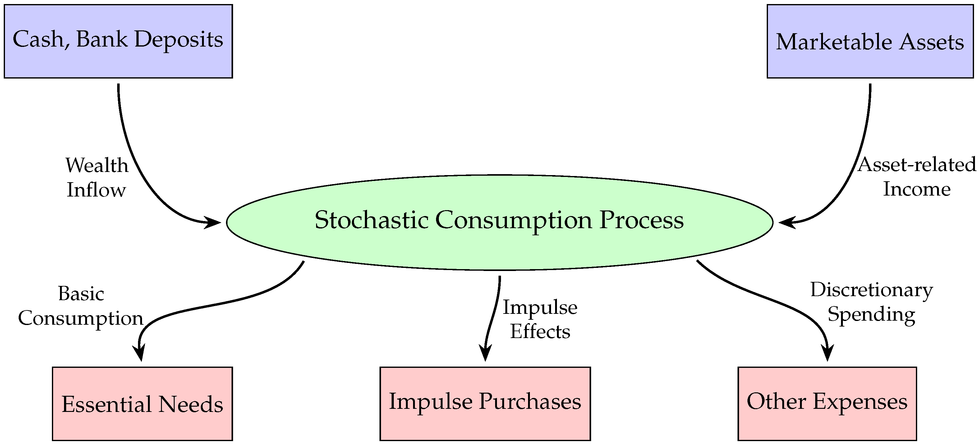
4.1. Stochastic Consumption Process

In relevant research, traditional consumption control strategies are usually assumed to be continuous in stochastic problems. However, a closer look at real-life consumption phenomena reveals that such strategies are not always as smooth and continuous as those in theoretical models.
In real-life scenarios, consumer behavior is influenced by numerous significant events. These events act as triggers, causing consumption control strategies to often experience abrupt changes. For example, during holidays, paydays, promotional activities, and large-scale exhibitions, consumers tend to engage in impulsive consumption. Such shifts cannot be accurately captured by traditional continuous control strategies. In fact, the consumption process aligns more closely with the characteristics of an impulse process, involving discontinuous and instantaneous changes at specific moments.
This section employs a stochastic differential variational inequality with impulses to model the stochastic consumption process. We introduce notations to describe the dynamics of a specific commodity’s consumption process over a given time frame.
Let z ( s ) denote the consumer’s wealth-related state variable at time s, which could incorporate elements such as cash, bank deposits, and marketable assets. Assume that consumers experience impulsive consumption at specific moments s j (e.g., holidays, paydays, sales, and promotional events). The impulse term is I j ( z ( s j ) ) = α j · y ( s j ) · β j , where α j is a proportionality factor indicating the degree of impulsive consumption at time s j , which may be related to consumer habits, psychological factors, etc. For impulsive consumers, α j may be relatively large; for conservative consumers, α j may be smaller. β j represents a random variable following a normal distribution with a mean of 1 and a variance of σ j 2 , which models the random characteristics of consumption impulses, i.e., even at the same wealth level, the magnitude of each consumption impulse may vary due to various random factors (such as mood at the time or chance encounters with products).
Let b 1 ( s , z ( s ) , v ( s ) ) represent the drift term, which could incorporate factors such as natural growth of wealth, regular income, and expenses. For example, it might include salary income and regular bill payments. The function b 2 ( s , z ( s ) , v ( s ) ) is the diffusion term, which models the impact of random factors on wealth, such as fluctuations in the stock market and inflation uncertainty. W ( s ) is a standard Brownian motion used to model market uncertainties.
The control variable v ( s ) represents the consumer’s consumption decision at time s, and U is the set of all possible consumption decisions. The inequality G ( s , ω , z ( s ) , v ( s ) ) , u v ( s ) 0 , u U , a . e . s δ , a . s . ω Ω is a variational-like condition that reflects the optimality or rationality of the consumption decision v ( s ) within the set U.
For the consumption process in stochastic environments, this issue can be expressed as the following stochastic system:
d z ( s ) = b 1 ( s , z ( s ) , v ( s ) ) d s + b 2 ( s , z ( s ) , v ( s ) ) d W ( s ) , s δ , s s j , Δ z ( s j ) = I j ( z ( s j ) ) , j = 1 , 2 , , m , z ( 0 ) = χ 0 + ϑ ( z ) , G ( s , ω , z ( s ) , v ( s ) ) , u v ( s ) 0 , u U , a . e . s δ , a . s . ω Ω .
Additionally, we present a stochastic consumption process as an illustration of the model (see Figure 1).

4.2. An Example from an Electrical Circuit Model

From [36], we know that differential variational inequalities (DVIs) can be used to model electrical circuits with (ideal) diodes. Assume that z 1 is the current through the inductor; z 2 is the voltage across the capacitor; ( v D i , i D i ) ( i = 1 , 2 , 3 , 4 ) is the voltage–current pair associated with the ith diode; and v is a sinusoidal voltage source. Setting z ( s ) = z 1 ( s ) , z 2 ( s ) T and v ( s ) = v 1 ( s ) , v 2 ( s ) , v 3 ( s ) , v 4 ( s ) T = i D 1 , v D 1 , v D 2 , i D 4 T . From [37], we can obtain that the electrical circuit with (ideal) diodes can be described as the following DVI:
d z ( s ) = A z ( s ) + B v ( s ) + f ( s ) d s , z ( 0 ) = χ 0 , Q z ( s ) + M v ( s ) , u v ( s ) 0 , u U , a . e . s δ , a . s . ω Ω ,
where A = 2 3 0 0 1 5 , B = 0 1 3 1 3 0 1 0 0 1 , f ( s ) = 2 sin ( 3 s π 3 ) , 0 T , χ 0 = ( 1 , 0 ) T , Q = 0 1 1 0 1 1 0 1 , M = 0 0 1 0 0 0 0 1 1 0 0 0 0 1 0 0 , U = v R n : 10 v 1 , v 2 10 , 0 v 3 , v 4 20 , δ = [ 0 , 1.5 ] .
We consider electrical circuits with (ideal) diodes in a nonlocal impulsive stochastic environment.
d z ( s ) = A z ( s ) + B v ( s ) + f ( s ) d s + C z ( s ) + D v ( s ) + g ( s ) d W ( s ) , s δ , s s j , Δ z ( s j ) = I j ( z ( s j ) ) , j = 1 , 2 , , m , z ( 0 ) = χ 0 + ϑ ( z ) , Q z ( s ) + M v ( s ) , u v ( s ) 0 , u U , a . e . s δ , a . s . ω Ω ,
where C = a 0 0 b , D = b b b b b b , g ( s ) = c sin ( s ) , 0 T , W ( s ) is a one-dimensional standard Brownian motion, ϑ ( z ) = α 0 1.5 z ( s ) d s is a continuous functional, and Δ z ( s j ) = ( β j , 0 ) T . Here, a , b , c R are diffusion coefficients related to z ( s ) , v ( s ) , and time s, respectively. β j R is the current impulse of the j-th impulse, which means only the current changes abruptly while the voltage remains unchanged.
It follows from Theorem 1 that (7) admits a unique solution z ( t ) , v ( t ) .

5. Conclusions

This study introduces an impulsive stochastic differential variational inequality that comprehensively integrates the impulsive stochastic differential equation and stochastic variational inequality. Through the application of the projection method, Itô calculus, and the Cauchy–Schwarz inequality, we prove the existence and uniqueness of the solution to (1) under relatively weak conditions. To demonstrate its practical relevance, we present two examples of consumption processes and electrical circuit models in a stochastic environment. Notably, Brownian motion has long been a central topic in the research of stochastic systems [38]. However, there remains a dearth of investigations into stochastic differential variational inequalities (SDVIs) driven by Brownian motion with impulsive behavior. Thus, our formulation of SDVIs incorporating Brownian-motion-driven impulses represents a significant and novel contribution to the field.

Author Contributions

Writing—original draft, W.L.; Writing—review & editing, K.L. All authors have read and agreed to the published version of the manuscript.

Funding

This research was funded by Guizhou University Introduced Talent Research Project (2022) No. 70 and Basic Research Project of Guizhou University (2023) No. 39.

Data Availability Statement

Data are contained within the article.

Conflicts of Interest

The authors declare no conflicts of interest.

References

  1. Drissi-Kaitouni, O. A variational inequality formulation of the dynamic traffic assignment problem. Eur. J. Oper. Res. 1993, 71, 188–204. [Google Scholar] [CrossRef]
  2. Facchinei, F.; Pang, J.S. Finite-Dimensional Variational Inequalities and Complementarity Problems; Springer: New York, NY, USA, 2003. [Google Scholar]
  3. Neittaanmäki, P.; Tiba, D. A variational inequality approach to constrained control problems for parabolic equations. Appl. Math. Optim. 1988, 17, 185–201. [Google Scholar] [CrossRef]
  4. Aubin, J.P.; Cellina, A. Differential Inclusions: Set-Valued Maps and Viability Theory; Springer: Berlin/Heidelberg, Germany, 1984. [Google Scholar]
  5. Pang, J.S.; Stewart, D.E. Differential variational inequalities. Math. Program. 2008, 113, 345–424. [Google Scholar] [CrossRef]
  6. Chen, X.; Wang, Z. Differential variational inequality approach to dynamic games with shared constraints. Math. Program. 2014, 146, 379–408. [Google Scholar] [CrossRef]
  7. Gwinner, J. On a new class of differential variational inequalities and a stability result. Math. Program. 2013, 139, 205–221. [Google Scholar] [CrossRef]
  8. Liu, Z.H.; Zeng, S.D. Differential variational inequalities in infinite Banach spaces. Acta Math. Sci. 2017, 37, 26–32. [Google Scholar] [CrossRef]
  9. Zeng, S.; Liu, Z.; Migorski, S. A class of fractional differential hemivariational inequalities with application to contact problem. Z. Angew. Math. Phys. 2018, 69, 36. [Google Scholar] [CrossRef]
  10. Cen, J.; Khan, A.A.; Motreanu, D.; Zeng, S. Inverse problems for generalized quasi-variational inequalities with application to elliptic mixed boundary value systems. Inverse Probl. 2022, 38, 065006. [Google Scholar] [CrossRef]
  11. Liu, Z.; Zeng, S.; Motreanu, D. Evolutionary problems driven by variational inequalities. J. Differ. Equ. 2016, 260, 6787–6799. [Google Scholar] [CrossRef]
  12. Hao, J.; Wang, J.; Lu, L. Coupled system of fractional hemivariational inequalities with applications. Optimization 2024, 73, 969–994. [Google Scholar] [CrossRef]
  13. Hao, J.; Li, M. A new class of fractional Navier–Stokes system coupled with multivalued boundary conditions. Commun. Nonlinear Sci. Numer. Simul. 2024, 136, 108098. [Google Scholar] [CrossRef]
  14. Hao, J.; Han, J.; Liu, Q. Existence and convergence analysis of second-order delay differential variational–hemivariational inequalities with memory terms. Nonlinear Anal. Real World Appl. 2025, 85, 104373. [Google Scholar] [CrossRef]
  15. Han, J.; Lu, L.; Zeng, S. Evolutionary variational–hemivariational inequalities with applications to dynamic viscoelastic contact mechanics. Z. Angew. Math. Phys. 2020, 71, 32. [Google Scholar] [CrossRef]
  16. Han, J.; Li, C.; Zeng, S. Applications of generalized fractional hemivariational inequalities in solid viscoelastic contact mechanics. Commun. Nonlinear Sci. Numer. Simul. 2022, 115, 106718. [Google Scholar] [CrossRef]
  17. Vetro, C.; Zeng, S. Regularity and Dirichlet problem for double-phase energy functionals of different power growth. J. Geom. Anal. 2024, 34, 105. [Google Scholar] [CrossRef]
  18. Zeng, S.; Bouach, A.; Haddad, T. On nonconvex perturbed fractional sweeping processes. Appl. Math. Optim. 2024, 89, 73. [Google Scholar] [CrossRef]
  19. Hao, X.; Liu, L.; Wu, Y. Mild solutions of impulsive semilinear neutral evolution equations in Banach spaces. J. Nonlinear Sci. Appl. 2016, 9, 6183–6194. [Google Scholar] [CrossRef]
  20. Sivasankaran, S.; Arjunan, M.M.; Vijayakumar, V. Existence of global solutions for second order impulsive abstract partial differential equations. Nonlinear Anal. Theory Methods Appl. 2011, 74, 6747–6757. [Google Scholar] [CrossRef]
  21. Nisar, K.S.; Vijayakumar, V. An analysis concerning approximate controllability results for second-order Sobolev-type delay differential systems with impulses. J. Inequalities Appl. 2022, 2022, 53. [Google Scholar] [CrossRef]
  22. Valliammal, N.; Jothimani, K.; Johnson, M.; Panda, S.K.; Vijayakumar, V. Approximate controllability analysis of impulsive neutral functional hemivariational inequalities. Commun. Nonlinear Sci. Numer. Simul. 2023, 127, 107560. [Google Scholar] [CrossRef]
  23. Liu, K.; Fečkan, M.; O’Regan, D.; Wang, J. (omega, c)-periodic solutions for time-varying non-instantaneous impulsive differential systems. Appl. Anal. 2022, 101, 5469–5489. [Google Scholar] [CrossRef]
  24. Liu, K.; Fečkan, M.; Wang, J.R. A class of (omega, T)-periodic solutions for impulsive evolution equations of Sobolev type. Bull. Iran. Math. Soc. 2022, 48, 2743–2763. [Google Scholar] [CrossRef]
  25. Ding, Y.; Liu, K. Periodic Solutions for Conformable Non-autonomous Non-instantaneous Impulsive Differential Equations. Math. Slovaca 2024, 74, 1489–1506. [Google Scholar] [CrossRef]
  26. Ding, Y.; Liu, K. Properties of the solutions to periodic conformable non-autonomous non-instantaneous impulsive differential equations. Electron. J. Differ. Equ. 2024, 2024, 1–22. [Google Scholar] [CrossRef]
  27. Rockafellar, R.T.; Wets, R.J.B. Stochastic variational inequalities: Single-stage to multistage. Math. Program. 2017, 165, 331–360. [Google Scholar] [CrossRef]
  28. Wang, R.; Kinra, K.; Mohan, M.T. Asymptotically autonomous robustness in probability of random attractors for stochastic Navier-Stokes equations on unbounded Poincaré domains. SIAM J. Math. Anal. 2023, 55, 2644–2676. [Google Scholar] [CrossRef]
  29. Wang, R.; Chen, P. Enhanced Mean Random Attractors for Nonautonomous Mean Random Dynamical Systems in Product Bochner Spaces. Commun. Math. Stat. 2024, 1–30. [Google Scholar] [CrossRef]
  30. Yang, M.; Lv, T.; Wang, Q. The averaging principle for Hilfer fractional stochastic evolution equations with Lévy noise. Fractal Fract. 2023, 7, 701. [Google Scholar] [CrossRef]
  31. Yang, M.; Huan, Q.; Cui, H.; Wang, Q. Hilfer fractional stochastic evolution equations on the positive semi-axis. Alex. Eng. J. 2024, 104, 386–395. [Google Scholar] [CrossRef]
  32. Zhang, Y.; Chen, T.; Huang, N.; Li, X. Euler scheme for solving a class of stochastic differential variational inequalities with some applications. Commun. Nonlinear Sci. Numer. Simul. 2023, 127, 107577. [Google Scholar] [CrossRef]
  33. Zeng, Y.; Zhang, Y.; Huang, N. A stochastic fractional differential variational inequality with Lévy jump and its application. Chaos Solitons Fractals 2024, 178, 114372. [Google Scholar] [CrossRef]
  34. Zhang, Y.; Chen, T.; Huang, N.; Li, X. Penalty method for solving a class of stochastic differential variational inequalities with an application. Nonlinear Anal. Real World Appl. 2023, 73, 103889. [Google Scholar] [CrossRef]
  35. Weng, H.Y.; Chen, T.; Huang, J.N.; O’Regan, D. A new class of fractional impulsive differential hemivariational inequalities with an application. Nonlinear Anal. Model. Control 2022, 27, 199–220. [Google Scholar] [CrossRef]
  36. Han, L.; Tiwari, A.; Camlibel, M.K.; Pang, J.S. Convergence of time-stepping schemes for passive and extended linear complementarity systems. SIAM J. Numer. Anal. 2009, 47, 3768–3796. [Google Scholar] [CrossRef]
  37. Haase, H.; Garbe, H.; Gerth, H. Grundlagen der Elektrotechnik; Schöneworth: Hannover, Germany, 2009. [Google Scholar]
  38. Ahmadian, D.; Ballestra, L.V.; Shokrollahi, F. A Monte-Carlo approach for pricing arithmetic Asian rainbow options under the mixed fractional Brownian motion. Chaos Solitons Fractals 2022, 158, 112023. [Google Scholar] [CrossRef]
Figure 1. Stochastic consumption process model.
Axioms 14 00603 g001
Disclaimer/Publisher’s Note: The statements, opinions and data contained in all publications are solely those of the individual author(s) and contributor(s) and not of MDPI and/or the editor(s). MDPI and/or the editor(s) disclaim responsibility for any injury to people or property resulting from any ideas, methods, instructions or products referred to in the content.

