An Inexact Nonsmooth Quadratic Regularization Algorithm

Abstract

The quadratic regularization technique is widely used in the literature for constructing efficient algorithms, particularly for solving nonsmooth optimization problems. We propose an inexact nonsmooth quadratic regularization algorithm for solving large-scale optimization, which involves a large-scale smooth separable item and a nonsmooth one. The main difference between our algorithm and the (exact) quadratic regularization algorithm is that it employs inexact gradients instead of the full gradients of the smooth item. Also, a slightly different update rule for the regularization parameters is adopted for easier implementation. Under certain assumptions, it is proved that the algorithm achieves a first-order approximate critical point of the problem, and the iteration complexity of the algorithm is $O\left({\epsilon }^{-2}\right)$. In the end, we apply the algorithm to solve LASSO problems. The numerical results show that the inexact algorithm is more efficient than the corresponding exact one in large-scale cases.

1. Introduction

Consider the following nonsmooth optimization problem:

$$\underset{x\in R^d}{min}f\left(x\right)+h\left(x\right),$$

(1)

where $f:R^d\to R$ is a continuously differentiable function and $h:R^d\to R\cup \{+\infty \}$ is a lower semi-continuous proper function (both f and h can be nonconvex). When $h\equiv 0$, the problem reduces to a smooth optimization. The trust-region-based algorithm is one of the classical methods for solving the problem, and it has attracted great attention in the literature since it was introduced. Comprehensive and systematical introductions can be found, for example, in book [1] and two novel variants in [2], which include regularization versions of the algorithm. By introducing a second-order nonlinear step-size control for the algorithm, Grapiglia et al. [3] proved the iteration complexity of the trust-region algorithm is $O\left({\epsilon }^{-3}\right)(0<\epsilon <1)$. Bergou et al. [4] used the scaled norms for the trust-region algorithm and a cubic adaptive regularization algorithm, and by introducing line-search into the algorithm, the iteration complexity of the algorithm was improved to $O\left({\epsilon }^{-3/2}\right)$. In cases where $f\equiv 0$ in problem (1), the nonsmooth trust-region algorithm and the nonsmooth regularization methods (based on general directional derivatives) have also been proposed and studied; see details, e.g., [5,6,7]. For more smooth/nonsmooth methods for solving these two kinds of optimizations, the readers are referred to [8,9,10] and references therein. In the composite case of problem (1) when f and h are convex, Lee et al. [11] proposed a proximal Newton method for solving the problem and established the global convergence of the algorithm. Kim et al. [12] introduced a nonsmooth trust-region algorithm for the problem, which employs the full gradients of f in each subproblem. For a more general case when $h:=g\circ c$, where g is convex and c is continuously differentiable, Cartis et al. [13] proposed both the nonsmooth trust-region algorithm and the quadratic regularization variants for solving the problem. The iteration complexities of these algorithms were proven to $O\left({\epsilon }^{-2}\right)$. For more generalized and improved nonsmooth trust-region-based algorithms for solving such problems, see, e.g., [14,15,16]. It is worth mentioning that the proximal gradient method is also a commonly used class of algorithms for solving this problem. They have been extensively studied and applied to problems such as (group) sparse optimization and constrained optimization. For more details, refer to [17,18,19,20,21] and their references.

We focus on the more general composite problem (1) (where both f and h can be nonconvex). Li et al. [22] proposed a monotone proximal gradient algorithm for solving the problem. Its sublinear convergence properties are established under the Kurdyka-Łojasiewicz condition. In particular, we note the work by Aravkin et al. [23], where the nonsmooth trust-region algorithm and the nonsmooth quadratic regularization algorithms were proposed and studied. Under certain conditions, they proved that the iteration complexities of both algorithms are $O\left({\epsilon }^{-2}\right)$. It should be noted that some of the aforementioned works related to the smooth term f all use the full gradients $\nabla f$ of f. To solve the following large-scale optimizations, we shall propose an algorithm that uses the inexact gradients of f instead of the full gradients. Specifically, we consider the following large-scale separable nonsmooth optimization problem:

$$\underset{x\in R^d}{min}f\left(x\right)+h\left(x\right):={\displaystyle \frac{1}{n}}\sum _{i=1}^n{f}_i\left(x\right)+h\left(x\right),$$

(2)

where each component function $f_i:R^d\to R$ is continuously differentiable ($i=1,2,\dots ,n$), $h:R^d\to R\cup \{+\infty \}$ is a proper and lower semi-continuous function, and $n\gg 1$ (i.e., n is very large). Such large-scale problems have broad applications in areas like machine learning, signal processing, image analysis and restoration, etc.; see, e.g., [24,25,26,27]. To reduce the computational complexity and memory usage in each iteration, some inexact techniques are applied in the algorithm design. For example, the incremental algorithms compute by processing data incrementally, typically one sample or a small batch at a time; see, e.g., [24]. Stochastic algorithms update estimates sequentially using stochastic batches of data; see, e.g., [25,26,27] and references therein. For solving problem (2), we propose an inexact nonsmooth quadratic regularization algorithm, which employs inexact gradients of f in the subproblems and also an account for nonsmooth function h (note that the inexact gradient of f includes sub-sampled gradient ${\displaystyle \frac{1}{|I_g|}}{\sum }_{i\in I_g}\nabla f_i$ of f as a special case, where $I_g$ is a sample collection from $I:=\{1,2,\dots ,n\}$; see Remark 4 for more details). The algorithm is actually an inexact version of the algorithm in ([23], Algorithm 6.1). The main difference between our algorithm and ([23], Algorithm 6.1) is that we employ inexact gradients of f, while the latter uses full gradients of f. Moreover, we adopt a different stopping criteria and slightly different update rules for the regularization parameters; see details in Remarks 1 and 2. Under certain conditions, we show that the iteration complexity of the algorithm is $O\left({\epsilon }^{-2}\right)$, which is similar to the result about the exact algorithm established in [23]. Finally, the algorithm is applied to solve LASSO problems, and numerical experiments show that in large-scale cases, the inexact algorithm is generally more efficient than the corresponding exact one.

The paper is organized as follows. The next section provides some necessary notions, notation and results. The main results are presented in Section 3, including the inexact nonsmooth quadratic regularization algorithm and the convergence analysis. Some numerical comparisons are illustrated in Section 4 for solving LASSO problems. The conclusion is given afterwards.

In addition, some useful notations are displayed in Table 1.

Table 1. Notations and descriptions.

Notation	Description
$\nabla f\left(x\right)$	gradient of function f at point x
$g\left(x\right)$	approximation of $\nabla f\left(x\right)$
$\widehat{\partial }h\left(x\right)$	Fréchet subdifferential of h at x
$\partial h\left(x\right)$	limiting subdifferential of h at x
$e_{\lambda h}\left(x\right)$	Moreau envelope of h at x with parameter $\lambda$
${\mathrm{prox}}_{\lambda h}\left(x\right)$	proximal mapping of h at x with parameter $\lambda$
${\lambda }_h$	* threshold of prox-boundedness of function h
${\sigma }_k$	regularization parameter in the k-th iteration
IG-QR	quadratic regularization algorithm employing inexact gradients
FG-QR	quadratic regularization algorithm employing full gradients

* The definition of the threshold of prox-boundedness is given in Definition 2.

2. Preliminaries

We gather some notation, notions, and results which will be used in this paper. For more details, the readers are referred to [1,23,28].

Let R denote the set of all real numbers and N denote the set of all non-negative integers. Let $\parallel ·\parallel$ and $⟨·,·⟩$ denote the ${\ell }_2$-norm and the inner product in Euclidean space $R^d$, respectively. The closed ball centered at 0 with radius $\delta >0$ is denoted by $\mathrm{B}(0,\delta )$; that is, $\mathrm{B}(0,\delta ):=\{x\in R^d:\parallel x\parallel ⩽\delta \}$. Let $x\in R^d$, and let $A\subseteq R^d$ be a nonempty subset. The distance from x to A is denoted by $\mathrm{dist}(x;A)$, which is defined by $\mathrm{dist}(x;A):={inf}_{a\in A}\left|\right|a-x\left|\right|$. Let $h:R^d\to \overline{R}:=R\cup \{+\infty \}$ be a lower semi-continuous proper function. As usual, $\mathrm{dom}h$ stands for the domain of h, that is,

$$\mathrm{dom}h:=\{x\in R^d:h\left(x\right)<+\infty \}.$$

The function h is said to be convex if the following inequality holds for any $x,y\in \mathrm{dom}h$

$$h(\lambda x+(1-\lambda \left)y\right)⩽\lambda h\left(x\right)+(1-\lambda )h\left(y\right)\forall \lambda \in (0,1).$$

Furthermore, h is said to be strongly convex with modulus $c>0$ if there exists a constant $c>0$ such that for any $x,y\in \mathrm{dom}h$, the following holds:

$$h(\lambda x+(1-\lambda )y)⩽\lambda h\left(x\right)+(1-\lambda )h\left(y\right)-{\displaystyle \frac{1}{2}}c\lambda (1-\lambda ){\parallel x-y\parallel }^2\forall \lambda \in (0,1).$$

For $\alpha \in R$, we use $L_{\alpha }\left(h\right)$ to stand for the $\alpha$-level set of h, that is,

$$L_{\alpha }\left(h\right):=\{x\in R^d:h\left(x\right)⩽\alpha \}.$$

If $L_{\alpha }\left(h\right)$ is bounded for any $\alpha \in R$, then h is said to be level-bounded. In the case when a lower semi-continuous proper function h is level-bounded, then the set ${argmin}_{x\in R^d}h\left(x\right):=\{z\in R^d:h\left(z\right)={min}_{x\in R^d}h\left(x\right)\}$ is nonempty and compact; see, e.g., ([28], Theorem 1.9).

The following concepts of the Moreau envelope and the proximal mapping of h can be found in ([23], Definition 2.1).

Definition 1 (Moreau Envelope and Proximal Mapping).

Let $x\in R^d$, and $\lambda >0$. The Moreau envelope $e_{\lambda h}\left(x\right)$ and the proximal mapping ${\mathrm{prox}}_{\lambda h}\left(x\right)$ of the function h at x are, respectively, defined by

$$e_{\lambda h}\left(x\right):=\underset{\omega }{inf}{\displaystyle \frac{1}{2\lambda }}{\parallel \omega -x\parallel }^2+h\left(\omega \right)={\lambda }^{-1}\underset{\omega }{inf}{\displaystyle \frac{1}{2}}{\parallel \omega -x\parallel }^2+\lambda h\left(\omega \right)$$

(3)

and

$${\mathrm{prox}}_{\lambda h}\left(x\right):=\underset{\omega }{argmin}{\displaystyle \frac{1}{2\lambda }}{\parallel \omega -x\parallel }^2+h\left(\omega \right)=\underset{\omega }{argmin}{\displaystyle \frac{1}{2}}{\parallel \omega -x\parallel }^2+\lambda h\left(\omega \right).$$

(4)

For a general lower semi-continuous proper function h, the set ${\mathrm{prox}}_{\lambda h}\left(x\right)$ can be empty or contain multiple elements. The range of parameter values for which the Moreau envelope of h admits a finite value is given by the following definition, which is taken from ([28], Definition 1.23).

Definition 2 (Prox-boundedness).

The function h is said to be prox-bounded if there exists a parameter $\lambda >0$ and at least one point $x\in R^d$ such that $e_{\lambda h}\left(x\right)>-\infty$. The threshold of prox-boundedness ${\lambda }_h$ of h is the supremum of all such $\lambda >0$.

It can be shown that the threshold of prox-boundedness of h is independent of the point x in the definition. In the special case when h is level-bounded, we see that ${\lambda }_h=+\infty$. A prox-bounded function exhibits the following properties ([28], Theorem 1.25).

Proposition 1.

Let $h:R^d\to \overline{R}$ be a prox-bounded function with proximal boundedness threshold ${\lambda }_h>0$. Then, for any $\lambda \in (0,{\lambda }_h)$ and $x\in R^d$, the following properties hold:

(i) ${\mathrm{prox}}_{\lambda h}\left(x\right)$ is a nonempty and compact set;

(ii) the function $(\lambda ,x)\mapsto e_{\lambda h}\left(x\right)$ is continuous, and as λ monotonically decreases to 0, $e_{\lambda h}\left(x\right)$ monotonically increases to $h\left(x\right)$.

We end this section with some optimality conditions for the nonsmooth optimization

$$\underset{x\in R^d}{min}\varphi \left(x\right),$$

(5)

where $\varphi :R^d\to \overline{R}$ is a lower semi-continuous proper function, which can be found in [23] or [28]. To this end, we first recall the following notions of the subgradient and subdifferential.

Definition 3 (Subgradient and Subdifferential).

Let $\overline{x}\in \mathrm{dom}\varphi$. A vector $v\in R^d$ is said to be a regular subgradient of ϕ at the point $\overline{x}$ if

$$\underset{x\to \overline{x}}{liminf}{\displaystyle \frac{\varphi \left(x\right)-\varphi \left(\overline{x}\right)-v^T(x-\overline{x})}{\Vert x-\overline{x}\Vert }}⩾0.$$

The set of all regular subgradients of ϕ at $\overline{x}$ is denoted by $\widehat{\partial }\varphi \left(\overline{x}\right)$, which is called the Fréchet subdifferential of ϕ at $\overline{x}$. Moreover, if there exist sequences $\left\{x_k\right\}\subset R^d$ and $\left\{v_k\right\}\subset \widehat{\partial }\varphi \left(x_k\right)$ satisfying $x_k\to \overline{x}$, $\varphi \left(x_k\right)\to \varphi \left(\overline{x}\right)$ and $v_k\to v$, then the vector v is called a general subgradient of ϕ at $\overline{x}$. The set of all general subgradients of ϕ at $\overline{x}$ is denoted by $\partial \varphi \left(\overline{x}\right)$, which is called the limiting subdifferential of ϕ at $\overline{x}$.

It is clear that $\widehat{\partial }\varphi \left(\overline{x}\right)\subseteq \partial \varphi \left(\overline{x}\right)$ for any $\overline{x}\in \mathrm{dom}\varphi$. In the case when $\varphi$ is convex, the Fréchet and limiting subdifferentials coincide with the subdifferential of convex analysis. Let $\varphi :=f+h$, where $f:R^d\to R$ is a continuously differentiable function, and let $\overline{x}\in \mathrm{dom}\varphi$. Then, $\partial \varphi \left(\overline{x}\right)=\nabla f\left(\overline{x}\right)+\partial h\left(\overline{x}\right)$. The following necessary optimality condition for (5) is well known.

Proposition 2.

Let $\overline{x}\in R^d$ be a local minimizer of ϕ. Then, $0\in \widehat{\partial }\varphi \left(\overline{x}\right)\subseteq \partial \varphi \left(\overline{x}\right)$. If ϕ is convex, then $\overline{x}$ is a global minimizer of ϕ.

A point $\overline{x}\in R^d$ is called a critical point of $\varphi$ if $0\in \partial \varphi \left(\overline{x}\right)$. In the next iteration complexity analysis, we need the following definition of approximate critical points, where $\mathrm{dist}(·;S):={inf}_{y\in S}\Vert y-·\Vert$ is the distance associated with $S\subset R^d$.

Definition 4.

Let $\epsilon >0$. A point $\overline{x}\in \mathrm{dom}\varphi$ is said to be a ε-approximate critical point of ϕ if $\mathrm{dist}(0;\partial \varphi \left(\overline{x}\right))⩽\epsilon$.

3. Inexact Nonsmooth Quadratic Regularization Algorithm

We consider the following large-scale separable nonsmooth optimization problem:

$$\underset{x\in R^d}{min}f\left(x\right)+h\left(x\right):={\displaystyle \frac{1}{n}}\sum _{i=1}^n{f}_i\left(x\right)+h\left(x\right),$$

(6)

where $n\gg 1$ (n is very large), each component function $f_i:R^d\to R$ is continuously differentiable $(i=1,2,\dots ,n)$, and $h:R^d\to \overline{R}$ is a lower semi-continuous proper function. Since n is very large, the computational cost of the (full) gradient of f becomes prohibitively expensive. To reduce the computational cost per iteration, we shall propose an inexact nonsmooth quadratic regularization algorithm (i.e., Algorithm 1) for solving problem (6), which employs approximate gradients of f instead of the full gradients in subproblems. The algorithm is actually an inexact version of the (exact) quadratic regularization algorithm proposed in ([23], Algorithm 6.1), for solving nonsmooth optimizations. In the k-th iteration, we construct an approximate model $\phi (·;x_k)+\psi (·;x_k)$ for $f(x_k+·)+h(x_k+·)$ at the iterate $x_k$ and then solve a quadratic regularization subproblem:

$$\underset{s}{min}m(s;x_k,{\sigma }_k):=\phi (s;x_k)+\psi (s;x_k)+{\displaystyle \frac{1}{2}}{\sigma }_k{\parallel s\parallel }^2,$$

(7)

where ${\sigma }_k>0$ is the regularization parameter.

We always make the following blanket assumption on the model.

Assumption 1 (Model Assumption).

For any $x\in R^d$,

(i) $\phi (·;x)$ is a linear function, which is defined by

$$\phi (s;x)=f\left(x\right)+g{\left(x\right)}^{T}s\forall s\in R^d,$$

(8)

where $g\left(x\right)\approx \nabla f\left(x\right)$;

(ii) $\psi (·;x):R^d\to \overline{R}$ is a lower semi-continuous proper function, and it satisfies $\psi (0;x)=h\left(x\right)$ and $\partial \psi (·;x)\left(0\right)=\partial h\left(x\right)$. Furthermore, $\psi (·;x)$ is uniformly prox-bounded; that is, ${\lambda }_{\psi }\in (0,+\infty )$ such that ${\lambda }_{\psi }<{\lambda }_{\psi (·;y)}$ for any $y\in R^d$.

Remark 1.

We note that Assumption 1 is similar to the corresponding one made in [23] for the (exact) nonsmooth quadratic regularization algorithm ([23], Algorithm 6.1), except the latter uses the full gradient of f in (8), that is, $g\left(x\right)=\nabla f\left(x\right)$ in (8). This means that both our algorithm (see Algorithm 1 below) and ([23], Algorithm 6.1) adopt a linear approximation φ of f in the quadratic regularization subproblem. The main difference lies in

• The first-order term of φ: Algorithm 1 uses the inexact gradient g as stated in (8), while ([23], Algorithm 6.1) uses the full gradient $\nabla f$, that is,

  $$\phi (·;x)=f\left(x\right)+\nabla f{\left(x\right)}^T(·)for any x\in R^d.$$
  We adopt a different tolerance that is easier to verify, which in turn requires a slightly modified update rule for the regularization parameters in Algorithm 1. These are specified as follows; see more explanations in Remark 2.
• Different stopping criterion: the stopping criterion of Algorithm 1 is $\parallel s_k\parallel <\epsilon$ (see Step 5 of Algorithm 1), while the stopping criterion of ([23], Algorithm 6.1) is

  $$f\left(x_k\right)+h\left(x_k\right)-p({\sigma }_{max};x_k)<{\epsilon }^2.$$
• Different update rule for $\left\{{\sigma }_k\right\}$: Algorithm 1 uses parameter ${\sigma }_{min}\in (0,{\lambda }_{\psi }^{-1})$ to ensure that all regularization parameters $\left\{{\sigma }_k\right\}$ have a positive lower bound, while ([23], Algorithm 6.1) does not use such a bound.

Below, we show that one can use proximal mappings to solve the quadratic regularization subproblems of Algorithm 1. To proceed, let $k\in N$. Noting the definition of subproblem (7) in the k-th iteration, we set

$$p({\sigma }_k;x_k):=\underset{s}{min}m(s;x_k,{\sigma }_k),$$

(9)

$$P({\sigma }_k;x_k):=\underset{s}{argmin}m(s;x_k,{\sigma }_k).$$

(10)

In view of (7) and (8), we can write

$$\begin{array}{cc}\hfill m(s;x_k,{\sigma }_k)& =f\left(x_k\right)+g{\left(x_k\right)}^{T}s+\psi (s;x_k)+{\displaystyle \frac{1}{2}}{\sigma }_k{\parallel s\parallel }^2\hfill \\ \hfill & ={\displaystyle \frac{1}{2}}{\sigma }_k\parallel s+{\sigma }_k^{-1}g\left(x_k\right){\parallel }^2+\psi (s;x_k)+f\left(x_k\right)-{\displaystyle \frac{1}{2}}{\sigma }_k^{-1}{\parallel g\left(x_k\right)\parallel }^2.\hfill \end{array}$$

(11)

Recalling (3) and (4), it holds from (9) and (10) that

$$p({\sigma }_k;x_k)=e_{{\sigma }_k^{-1}\psi (·;x_k)}(-{\sigma }_k^{-1}g\left(x_k\right))+f\left(x_k\right)-{\displaystyle \frac{1}{2}}{\sigma }_k^{-1}{\parallel g\left(x_k\right)\parallel }^2$$

(12)

and

$$P({\sigma }_k;x_k)=\underset{s}{argmin}{\displaystyle \frac{1}{2}}{\sigma }_k{\parallel s+{\sigma }_k^{-1}g\left(x_k\right)\parallel }^2+\psi (s;x_k)={\mathrm{prox}}_{{\sigma }_k^{-1}\psi (·;x_k)}(-{\sigma }_k^{-1}g\left(x_k\right)).$$

(13)

Noting that $\phi (·;x)$ is a linear function, it is easy to verify that ${\lambda }_{\psi (·;x)}$ is also the threshold of the prox-boundedness of $\phi (·;x)+\psi (·;x)$. Thus, the following result is immediate from Proposition 1(i).

Proposition 3.

Let $x\in R^d$ and ${\sigma }^{-1}\in (0,{\lambda }_{\psi (·;x)})$. Then, $P(\sigma ;x)$ is a nonempty and compact set.

By Assumption 1 and (13), the following decrease is guaranteed by the proximal gradient method.

Lemma 1.

Let $x\in \mathrm{dom}h$ and ${\sigma }^{-1}\in (0,{\lambda }_{\psi (·;x)})$. Then, we have

$$f\left(x\right)+h\left(x\right)-(\phi (s;x)+\psi (s;x))⩾{\displaystyle \frac{1}{2}}\sigma {\parallel s\parallel }^2\forall s\in P(\sigma ;x).$$

(14)

Below, we present the inexact nonsmooth quadratic regularization algorithm for solving problem (6), where the parameter ${\sigma }_{min}\in (0,{\lambda }_{\psi }^{-1})$.

Algorithm 1 Inexact Nonsmooth Quadratic Regularization Algorithm

1: Input: Choose $0<{\sigma }_{min}<{\sigma }_0$, $0<{\eta }_1⩽{\eta }_2<1$, $0<{\gamma }_3⩽1<{\gamma }_1⩽{\gamma }_2$, $\epsilon >0$. 2: Choose an initial point $x_0\in \mathrm{dom}h$, compute $f\left(x_0\right)+h\left(x_0\right)$. 3: for $k=0,1,\dots$do 4:  Solve the subproblem (7) to obtain $s_k\in P({\sigma }_k;x_k)$. 5:  If $\parallel s_k\parallel <\epsilon$, then stop and output $x_k$. 6:  Compute $${\rho }_k:={\displaystyle \frac{f\left(x_k\right)+h\left(x_k\right)-(f(x_k+s_k)+h(x_k+s_k))}{\phi (0;x_k)+\psi (0;x_k)-(\phi (s_k;x_k)+\psi (s_k;x_k))}}.$$ 7:  Set $x_{k+1}=\left\{\begin{array}{cc}{x}_k+s_k\hfill & \mathrm{if}{\rho }_k⩾{\eta }_1,\hfill \\ x_k\hfill & \mathrm{otherwise}.\hfill \end{array}\right.$ 8:  Update the regularization parameter $${\sigma }_{k+1}\in \left\{\begin{array}{cc}[max\{{\sigma }_{min},{\gamma }_3{\sigma }_k\},{\sigma }_k]\hfill & \mathrm{if}{\rho }_k⩾{\eta }_2\left(\mathrm{very}\mathrm{successful}\mathrm{iteration}\right),\hfill \\ [{\sigma }_k,{\gamma }_1{\sigma }_k]\hfill & \mathrm{if}{\eta }_1⩽{\rho }_k<{\eta }_2\left(\mathrm{successful}\mathrm{iteration}\right),\hfill \\ [{\gamma }_1{\sigma }_k,{\gamma }_2{\sigma }_k]\hfill & \mathrm{if}{\rho }_k<{\eta }_1\left(\mathrm{unsuccessful}\mathrm{iteration}\right).\hfill \end{array}\right.$$ 9:  Set $k=k+1$ and go to step 3. 10: end for

Remark 2.

Compared to ([23], Algorithm 6.1), we adopt a slightly different update rule for the regularization parameters at very successful iterations. This is because we use a different tolerance $\parallel s_k\parallel <\epsilon$ in Algorithm 1, which is easier to be verified than the tolerance $\xi ({\sigma }_{max};x_k):=f\left(x_k\right)+h\left(x_k\right)-p({\sigma }_{max};x_k)<{\epsilon }^2$ used in [23]. This leads to the necessity of the update rule when we study the iteration complexity of Algorithm 1 in what follows. In addition, we note that just like ([23], Algorithm 6.1), there may be iterations of Algorithm 1 where ${\sigma }_k^{-1}⩾{\lambda }_{\psi (·;x_k)}$. At such iterations, ${\sigma }_k$ is increased, and then after a finite number of such increases, there holds that ${\sigma }_k^{-1}<{\lambda }_{\psi (·;x_k)}$.

Similar to the (exact) quadratic regularization algorithm in ([23], Algorithm 6.1), we always make the following step assumption.

Assumption 2 (Step Assumption).

There exists ${\kappa }_{\mathrm{m}}>0$ such that for all k,

$$|f(x_k+s_k)+h(x_k+s_k)-\phi (s_k;x_k)-\psi (s_k;x_k)|⩽{\kappa }_{\mathrm{m}}{\parallel s_k\parallel }^2.$$

(15)

Remark 3.

Let $k\in N$, and let $\psi (s;x_k)$ be defined as $\psi (s;x_k):=h(x_k+s)$. If $\nabla f$ is Lipschitz continuous with constant $L>0$ and there exist constants $C>0$ such that for any $x\in R^d$,

$$\parallel \nabla f\left(x_k\right)-g\left(x_k\right)\parallel ⩽C\parallel s_k\parallel ,$$

(16)

then Assumption 2 is satisfied. In fact, in this case,

$$|f(x_k+s_k)+h(x_k+s_k)-\phi (s_k;x_k)-\psi (s_k;x_k)|=|f(x_k+s_k)-\phi (s_k;x_k)|.$$

By the mean value theorem, there exists ${\overline{x}}_{k,1}$ on the line segment connecting $x_k+s_k$ and $x_k$ such that

$$f(x_k+s_k)=f\left(x_k\right)+\nabla f{\left({\overline{x}}_{k,1}\right)}^T{s}_k.$$

From the definition of φ and (16), we have

$$\begin{array}{cc}\hfill |f(x_k+s_k)-\phi (s_k;x_k)|& ⩽\parallel \nabla f\left({\overline{x}}_{k,1}\right)-\nabla f\left(x_k\right)\parallel ·\parallel s_k\parallel +\parallel \nabla f\left(x_k\right)-g\left(x_k\right)\parallel ·\parallel s_k\parallel \hfill \\ \hfill & ⩽(L+C)\parallel s_k{\parallel }^2.\hfill \end{array}$$

Thus, Assumption 2 holds with ${\kappa }_{\mathrm{m}}:=L+C$. Additionally, when $h=g\circ c$, where $c:R^d\to R^l$ has a Lipschitz continuous Jacobian and $g:R^l\to R$ is Lipschitz continuous, the above condition $\psi (s;x_k)=h(x_k+s)$ can be replaced by $\psi (s;x_k)=g(c\left(x_k\right)+\nabla c{\left(x_k\right)}^{T}s)$, and Assumption 2 is still satisfied.

Regarding the sequence of regularization parameters $\left\{{\sigma }_k\right\}$, the following important property holds, where

$${\sigma }_{\mathrm{succ}}:=max\{{\displaystyle \frac{1}{{\lambda }_{\psi }}},{\displaystyle \frac{2{\kappa }_{\mathrm{m}}}{1-{\eta }_2}}\}>0.$$

Lemma 2.

If Algorithm 1 does not terminate at the k-th iteration and the regularization parameter satisfies ${\sigma }_k⩾{\sigma }_{\mathrm{succ}}$, then the k-th iteration is very successful, and ${\sigma }_{k+1}⩽{\sigma }_k$.

Proof of Lemma 2.

Let ${\sigma }_k⩾{\sigma }_{\mathrm{succ}}$, and let $x_k$ and $s_k$ be the corresponding iteration point and direction, respectively. Since Algorithm 1 does not terminate in finite steps, we have $s_k\ne 0$. Combining Assumption 2 and (14), we obtain

$$|{\rho }_k-1|={\displaystyle \frac{|f(x_k+s_k)+h(x_k+s_k)-(\phi (s_k;x_k)+\psi (s_k;x_k))|}{\phi (0;x_k)+\psi (0;x_k)-(\phi (s_k;x_k)+\psi (s_k;x_k))}}⩽{\displaystyle \frac{{\kappa }_{\mathrm{m}}{\parallel s_k\parallel }^2}{\frac{1}{2}{\sigma }_k{\parallel s_k\parallel }^2}}={\displaystyle \frac{2{\kappa }_{\mathrm{m}}}{{\sigma }_k}}.$$

From the definition of ${\sigma }_{\mathrm{succ}}$ and ${\sigma }_k⩾{\sigma }_{\mathrm{succ}}$, we have $|{\rho }_k-1|⩽1-{\eta }_2$. Noting that ${\rho }_k>0$ and $0<{\eta }_2<1$, it follows that ${\rho }_k⩾{\eta }_2$. By the definition of Algorithm 1, the k-th iteration is very successful, and ${\sigma }_{k+1}⩽{\sigma }_k$. □

Lemma 2 and the definition of Algorithm 1 indicate that the regularization parameters $\left\{{\sigma }_k\right\}$ generated by the algorithm have positive lower and upper bounds, i.e.,

$${\sigma }_{min}⩽{\sigma }_k⩽{\sigma }_{max}\forall k\in N,$$

(17)

where ${\sigma }_{max}:=max\{{\sigma }_0,{\gamma }_2{\sigma }_{\mathrm{succ}}\}$. Next, we show the iteration complexity of Algorithm 1. To this end, let $k\left(\epsilon \right)$ represent the number of iterations such that the termination condition $\parallel s_k\parallel <\epsilon$ is satisfied. Define the sets of all successful iterations and all unsuccessful iterations as

$$\mathcal{S}\left(\epsilon \right):=\{k<k\left(\epsilon \right):{\rho }_k⩾{\eta }_1\}\mathrm{and}\mathcal{U}\left(\epsilon \right):=\{k<k\left(\epsilon \right):{\rho }_k<{\eta }_1\}.$$

Let $\left|J\right|$ stand for the cardinality of the index subset $J\subseteq N$. The following lemma gives estimates about the cardinalities of $\mathcal{S}\left(\epsilon \right)$ and $\mathcal{U}\left(\epsilon \right)$, respectively. We note that the estimation method is similar to the complexity analysis of the classical regularization algorithm by Cartis et al. [13] or that of the nonsmooth quadratic regularization algorithm in [23].

Lemma 3.

Suppose that $f\left(x_k\right)+h\left(x_k\right)⩾{(f+h)}_{\mathbf{low}}$ for all $k\in N$. Then, the following estimates hold:

$$\left|\mathcal{S}\left(\epsilon \right)\right|⩽{\displaystyle \frac{2((f+h)\left(x_0\right)-{(f+h)}_{\mathbf{low}})}{{\eta }_1{\sigma }_{min}{\epsilon }^2}}=O\left({\epsilon }^{-2}\right)$$

(18)

and

$$\left|\mathcal{U}\left(\epsilon \right)\right|⩽{log}_{{\gamma }_1}({\sigma }_{max}/{\sigma }_0)+|\mathcal{S}\left(\epsilon \right)\left|\right|{log}_{{\gamma }_1}{\gamma }_3|=O\left({\epsilon }^{-2}\right).$$

(19)

Proof of Lemma 3.

Let $k\in \mathcal{S}\left(\epsilon \right)$. By the definition of Algorithm 1 and (14), there holds that

$$\begin{array}{cc}\hfill f\left(x_k\right)+h\left(x_k\right)-f(x_k+s_k)-h(x_k+s_k)& ⩾{\eta }_1(\phi (0;x_k)+\psi (0;x_k)-(\phi (s_k;x_k)+\psi (s_k;x_k)\left)\right)\hfill \\ \hfill & ⩾{\displaystyle \frac{1}{2}}{\eta }_1{\sigma }_k{\parallel s_k\parallel }^2⩾{\displaystyle \frac{{\sigma }_{min}}{2}}{\eta }_1{\epsilon }^2.\hfill \end{array}$$

Summing up the above inequalities over all $k\in \mathcal{S}\left(\epsilon \right)$, we get that

$$\sum _{k\in \mathcal{S}\left(\epsilon \right)}(f+h)\left(x_k\right)-(f+h)\left(x_{k+1}\right)⩾\left|\mathcal{S}\left(\epsilon \right)\right|{\displaystyle \frac{{\sigma }_{min}}{2}}{\eta }_1{\epsilon }^2.$$

Noting that the sequence $\{f\left(x_k\right)+h\left(x_k\right)\}$ is decreasing and bounded from below by ${(f+h)}_{\mathbf{low}}$, it follows that

$$(f+h)\left(x_0\right)-{(f+h)}_{\mathbf{low}}⩾\left|\mathcal{S}\left(\epsilon \right)\right|{\displaystyle \frac{{\sigma }_{min}}{2}}{\eta }_1{\epsilon }^2,$$

which implies (18). Note that each unsuccessful iteration increases the regularization parameter by at least a factor of ${\gamma }_1$, while each successful iteration reduces the regularization parameter by at most a factor of ${\gamma }_3$ ($0<{\gamma }_3⩽1<{\gamma }_1$). Therefore, we have

$${\sigma }_{max}⩾{\sigma }_{k\left(\epsilon \right)-1}⩾{\sigma }_0{\gamma }_1^{\left|\mathcal{U}\right(\epsilon \left)\right|}{\gamma }_3^{\left|\mathcal{S}\right(\epsilon \left)\right|},$$

and so

$${log}_{{\gamma }_1}({\sigma }_{max}/{\sigma }_0)⩾|\mathcal{U}\left(\epsilon \right)|{log}_{{\gamma }_1}{\gamma }_1+\left|\mathcal{S}\left(\epsilon \right)\right|{log}_{{\gamma }_1}{\gamma }_3.$$

Thus, (19) is valid, completing the proof. □

The following iteration complexity for Algorithm 1 is immediate from the above lemma.

Theorem 1.

Under the assumptions made in Lemma 3, we have $k\left(\epsilon \right)=O\left({\epsilon }^{-2}\right)$.

The following proposition provides some conditions to ensure that Algorithm 1 terminates at an approximate stationary point.

Proposition 4.

Suppose that Algorithm 1 terminates at the k-th iteration, that is, $\parallel s_k\parallel <\epsilon$. Suppose further that $\nabla f$ is Lipschitz continuous with constant $L>0$, $\psi (·;x_k):=h(x_k+·)$, and

$$\parallel \nabla f\left(x_k\right)-g\left(x_k\right)\parallel ⩽c_k\parallel s_k\parallel$$

(20)

holds with some $c_k>0$. Then, $x_k+s_k$ is a $({\sigma }_k+c_k+L)\epsilon$-approximate critical point of $f+h$.

Proof of Proposition 4.

By assumption and the definition of $s_k$, we have

$$0\in g\left(x_k\right)+\partial \psi (·;x_k)\left(s_k\right)+{\sigma }_k{s}_k.$$

Thus,

$$\begin{array}{cc}\hfill -{\sigma }_k{s}_k+(\nabla f(x_k+s_k)-g\left(x_k\right))& \in \nabla f(x_k+s_k)+\partial \psi (·;x_k)\left(s_k\right)\hfill \\ \hfill & =\nabla f(x_k+s_k)+\partial h(x_k+s_k)\hfill \\ \hfill & =\partial (f+h)(x_k+s_k).\hfill \end{array}$$

Noting that

$$\parallel -{\sigma }_k{s}_k+(\nabla f(x_k+s_k)-g\left(x_k\right))\parallel ⩽{\sigma }_k\parallel s_k\parallel +\parallel \nabla f(x_k+s_k)-g\left(x_k\right)\parallel$$

and

$$\begin{array}{c}\hfill \parallel \nabla f(x_k+s_k)-g\left(x_k\right)\parallel ⩽\parallel \nabla f(x_k+s_k)-\nabla f\left(x_k\right)\parallel +\parallel \nabla f\left(x_k\right)-g\left(x_k\right)\parallel ,\end{array}$$

we get that

$$\mathrm{dist}(0;\partial (f+h)(x_k+s_k))<({\sigma }_k+c_k+L)\epsilon .$$

By definition, this implies that $x_k+s_k$ is a $({\sigma }_k+c_k+L)\epsilon$-approximate critical point of $f+h$. The proof is complete. □

Remark 4.

Noting that $f:={\displaystyle \frac{1}{n}}{\sum }_{i=1}^n{f}_i$ is separable, one can adopt sub-sampled inexact gradient $g:={\displaystyle \frac{1}{|I_g|}}{\sum }_{i\in I_g}\nabla f_i$, where $I_g$ is a sample collection with or without replacement from $I:=\{1,2,\dots ,n\}$. There are some methods to provide sufficient sample sizes to guarantee that the sub-sampled inexact gradient g approximates $\nabla f$ in a probabilistic way; for more details, the readers are referred to, for example, ([29], Lemma 3). In the next section, we always adopt sub-sampled inexact gradients in implementing Algorithm 1.

4. Implementation and Numerical Results

We consider the following LASSO problem:

$$\underset{x\in R^d}{min}{\displaystyle \frac{1}{2n}}{\parallel Ax-b\parallel }_2^2+{\mu \parallel x\parallel }_1={\displaystyle \frac{1}{2n}}\sum _{i\in I}{(A_{i}x-b_i)}^2+\mu {\parallel x\parallel }_1,$$

(21)

where $A\in R^{n\times d}$ is a given design matrix, $I:=\{1,2,\dots ,n\}$, ${\parallel ·\parallel }_1$ is the ${\ell }_1$-norm in Euclidean space $R^d$, $A_i$ is the i-th row vector of matrix A, and $b\in R^n$ is the observed noisy data. This model aims to recover sparse coefficient x, which is a popular model used in high-dimensional data analysis, sparse feature selection, and dimensionality reduction, etc.; see, e.g., for example [23,30]. All numerical experiments are implemented in Python 3.11.7 and on a Lenovo 90M2CTO1WW PC (Intel(R) Core(TM) i5-9500, 3.00 GHz, 8.00 GB (2667 MHz) RAM).

In particular, we generate a sparse vector $x_{\mathrm{true}}\in R^d$ which contains mostly zeros and 10 values of $\pm 1$, where both the index of the nonzero entry and $\pm 1$ are randomly generated. We generate the matrix $A\in R^{n\times d}$ using i.i.d. (independent and identically distributed) random entries, where each entry is sampled from the standard normal distribution $\mathcal{N}(0,1)$, and $b:=A{x}_{\mathrm{true}}+ϵ$, where $ϵ\sim \mathcal{N}(0,0.01)$. The parameter $\mu$ of problem (21) is set by $\mu :=0.01$.

We apply Algorithm 1 to solve problem (21), where the subproblem (7) is set as

$$\underset{s}{min}m(s;x_k,{\sigma }_k):=f\left(x_k\right)+g{\left(x_k\right)}^{T}s+\mu \parallel x_k{+s\parallel }_1+{\displaystyle \frac{1}{2}}{\sigma }_k{\parallel s\parallel }_2^2\forall k\in N$$

($f(·):={\displaystyle \frac{1}{2n}}{\sum }_{i=1}^n{(A_i(·)-b_i)}^2$). Two versions of Algorithm 1 are considered as follows.

(1)

Algorithm 1 employs inexact gradients, which are referred to as IG-QR for short. That is, $g\left(x_k\right):={\displaystyle \frac{1}{|I_g|}}{\sum }_{i\in I_g}(A_i{x}_k-b_i)A_i^T$ in the subproblem (11) in the k-th iteration, where $I_g$ is an index subset randomly sampled from I without replacement. The sampling technique is referred to the stochastic gradient algorithm, for example [25,26,31]. More specifically, we set the sampling ratio at $10\%$.

(2)

Algorithm 1 employs full gradients, which are referred to as FG-QR for short. That is, $g\left(x_k\right):=\nabla f\left(x_k\right)={\displaystyle \frac{1}{\left|I\right|}}{\sum }_{i\in I}(A_i{x}_k-b_i)A_i^T$ in the subproblem (11) in the k-th iteration.

In all implementations, the initial points $x_0$ are drawn from a standard normal distribution, which is denoted as $x_0\sim \mathcal{N}(0,1)$. The parameter values are set as follows: ${\sigma }_0:=10$, ${\sigma }_{\min }:=8.0$, ${\eta }_1:=0.25$, ${\eta }_2:=0.75$, ${\gamma }_1:=2.0$, ${\gamma }_2:=3.0$, ${\gamma }_3:=0.5$ and $\epsilon :=0.001$.

Table 2 reports the numerical results of FG-QR and IG-QR across various dimensions. For the special case when $n=\mathrm{150,000}$, $d=500$, we performed 20 independent trials. In each trail, we regenerate a sparse vector $x_{\mathrm{true}}$, data pairs $(A,b)$ and initial points $x_0$. As illustrated in Figure 1, we compare the objective function values of FG-QR and IG-QR versus CPUtime across 20 independent trials. Meanwhile, Figure 2 shows $x_{\mathrm{true}}$ alongside the recovered coefficients obtained by FG-QR and IG-QR. We observe from the numerical results that FG-QR and IG-QR achieve comparable accuracy in recovering $x_{\mathrm{true}}$. Notably, although IG-QR requires more iterations, it outperforms FG-QR in terms of less CPUtime. This observation shows the superiority of IG-QR especially when dealing with high-dimensional problems.

Table 2. Numerical results across various dimensions, where O-v = $f\left(x\right)+{\mu \parallel x\parallel }_1$, R-e = $\parallel x-x_{\mathrm{true}}\parallel /\parallel x_{\mathrm{true}}\parallel$, I-k is the number of iterations, and T-s is the CPU time (in seconds).

Dimensions		True	FG-QR				IG-QR
n	d	O-v	O-v	R-e	I-k	T-s	O-v	R-e	I-k	T-s
100,000	200	0.105016	0.104550	0.011752	49	4.601011	0.104558	0.012024	51	2.642049
100,000	500	0.105025	0.104531	0.011712	48	12.862375	0.104545	0.011038	52	7.583251
100,000	800	0.104999	0.104523	0.012177	50	20.439099	0.104526	0.011822	57	13.037192
150,000	200	0.104985	0.104511	0.011667	49	5.919224	0.104521	0.011709	50	3.301263
150,000	500	0.105012	0.104526	0.012019	50	13.428264	0.104523	0.011853	52	8.217642
150,000	800	0.105001	0.104528	0.011814	50	25.827659	0.104539	0.011963	56	16.310059
200,000	200	0.105009	0.104548	0.011770	49	7.683134	0.104547	0.011395	50	4.764928
200,000	500	0.104975	0.104503	0.011600	49	26.579966	0.104510	0.011754	52	15.295921
200,000	800	0.105024	0.104552	0.012110	50	39.642553	0.104554	0.011776	55	24.811985

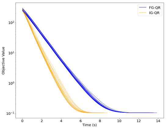
Figure 1. Numerical performance of FG-QR and IG-QR, when $n=\mathrm{150,000}$, $d=500$, was evaluated across 20 independent trials.

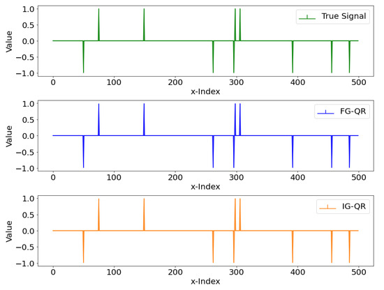
Figure 2. $x_{\mathrm{true}}$ alongside the recovered coefficients obtained by FG-QR and IG-QR in a trial.

5. Conclusions

This paper proposes an inexact nonsmooth quadratic regularization algorithm based on approximate gradients. The primary objective is to reduce the computational cost per iteration when dealing with large-scale problems. We have shown that the iteration complexity of this algorithm is comparable to that of the corresponding algorithm using full gradients. When the approximate gradient meets certain conditions, an approximate first-order stationary point of the original problem can be achieved. To verify the efficiency of the algorithm in practical applications, we apply it to solve large-scale LASSO problems. Numerical results indicate that Algorithm 1 outperforms the exact algorithm using full gradients, especially when dealing high-dimensional LASSO problems. Note that in general, it is difficult to get an exact solution of the subproblem. Our future work will consider algorithms for the inexact solutions of subproblems as well as some specific computational issues. Additionally, we will consider cubic regularization methods and more general nonlinear step-size control approaches.

References

- Conn, A.R.; Gould, N.I.M.; Toint, P.L. Trust Region Methods, 1st ed.; SIAM: Philadelphia, PA, USA, 2000; pp. 113–434. ISBN 978-0-89871-985-7. [Google Scholar]
- Toint, P.L. Nonlinear stepsize control, trust regions and regularizations for unconstrained optimization. Optim. Method Softw. 2013, 28, 82–95. [Google Scholar] [CrossRef][Green Version]
- Grapiglia, G.N.; Yuan, J.Y.; Yuan, Y.X. Nonlinear stepsize control algorithms: Complexity bounds for first- and second-order optimality. J. Optim. Theory Appl. 2016, 171, 980–997. [Google Scholar] [CrossRef]
- Bergou, E.H.; Diouane, Y.; Gratton, S. A line-search algorithm inspired by the adaptive cubic regularization framework and complexity analysis. J. Optim. Theory Appl. 2018, 178, 885–913. [Google Scholar] [CrossRef]
- Dennis, J.E., Jr.; Li, S.B.B.; Tapia, R.A. A unified approach to global convergence of trust region methods for nonsmooth optimization. Math. Program. 1995, 68, 319–346. [Google Scholar] [CrossRef][Green Version]
- Qi, L.Q.; Sun, J. A trust region algorithm for minimization of locally Lipschitzian functions. Math. Program. 1994, 66, 25–43. [Google Scholar] [CrossRef]
- Mashreghi, Z.; Nasri, M. Bregman distance regularization for nonsmooth and nonconvex optimization. Can. Math. Bul.-Bul. Can. Math. 2024, 67, 415–424. [Google Scholar] [CrossRef]
- Wang, X.M. Subgradient algorithms on Riemannian manifolds of lower bounded curvatures. Optimization 2018, 67, 179–194. [Google Scholar] [CrossRef]
- Wang, J.H.; Wang, X.M.; Li, C.; Yao, J.C. Convergence analysis of gradient algorithms on Riemannian manifolds without curvature constraints and application to Riemannian Mass. SIAM J. Optim. 2021, 31, 172–199. [Google Scholar] [CrossRef]
- Sun, W.M.; Liu, H.W.; Liu, Z.X. A regularized limited memory subspace minimization conjugate gradient method for unconstrained optimization. Numer. Algorithms 2023, 94, 1919–1948. [Google Scholar] [CrossRef]
- Lee, J.D.; Sun, Y.K.; Saunders, M.A. Proximal Newton-type methods for minimizing composite functions. SIAM J. Optim. 2014, 24, 1420–1443. [Google Scholar] [CrossRef]
- Kim, D.; Sra, S.; Dhillon, I. A scalable trust-region algorithm with application to mixed-norm regression. In Proceedings of the 27th International Conference on Machine Learning (ICML 2010), Haifa, Israel, 21–24 June 2010; pp. 519–526. [Google Scholar]
- Cartis, C.; Gould, N.I.M.; Toint, P.L. On the evaluation complexity of composite function minimization with applications to nonconvex nonlinear programming. SIAM J. Optim. 2011, 21, 1721–1739. [Google Scholar] [CrossRef]
- Chen, Z.A.; Milzarek, A.; Wen, Z.W. A trust-region method for nonsmooth nonconvex optimization. J. Comput. Math. 2023, 41, 683–716. [Google Scholar] [CrossRef]
- Liu, R.Y.; Pan, S.H.; Wu, Y.Q.; Yang, X.Q. An inexact regularized proximal Newton method for nonconvex and nonsmooth optimization. Comput. Optim. Appl. 2024, 88, 603–641. [Google Scholar] [CrossRef]
- Bolte, J.; Sabach, S.; Teboulle, M. Proximal alternating linearized minimization for nonconvex and nonsmooth problems. Math. Program. 2014, 146, 459–494. [Google Scholar] [CrossRef]
- Fukushima, M.; Mine, H. A generalized proximal point algorithm for certain non-convex minimization problems. Int. J. Syst. Sci. 1981, 12, 989–1000. [Google Scholar] [CrossRef]
- Tseng, P. On accelerated proximal gradient methods for convex-concave optimization. SIAM J. Optim. 2008, 2, 1–20. [Google Scholar]
- Tseng, P.; Yun, S. Block-coordinate gradient descent method for linearly constrained nonsmooth separable optimization. J. Optim. Theory Appl. 2009, 140, 513–535. [Google Scholar] [CrossRef]
- Nesterov, Y. Gradient methods for minimizing composite functions. Math. Program. 2013, 140, 125–161. [Google Scholar] [CrossRef]
- Wu, Q.Q.; Peng, D.T.; Zhang, X. Continuous exact relaxation and alternating proximal gradient algorithm for partial sparse and partial group sparse optimization problems. J. Sci. Comput. 2024, 100, 20. [Google Scholar] [CrossRef]
- Li, H.; Lin, Z.C. Accelerated proximal gradient methods for nonconvex programming. In Proceedings of the 29th International Conference on Neural Information Processing Systems (NIPS’15), Montreal, QC, Canada, 7–12 December 2015; pp. 379–387. [Google Scholar]
- Aravkin, A.Y.; Baraldi, R.; Orban, D. A proximal quasi-Newton trust-region method for nonsmooth regularized optimization. SIAM J. Optim. 2022, 32, 900–929. [Google Scholar] [CrossRef]
- Yang, D.; Wang, X.M. Incremental subgradient algorithms with dynamic step sizes for separable convex optimizations. Math. Meth. Appl. Sci. 2023, 46, 7108–7124. [Google Scholar] [CrossRef]
- Robbins, H.; Monro, S. A stochastic approximation method. Ann. Math. Statist. 1951, 22, 400–407. [Google Scholar] [CrossRef]
- Franchini, G.; Porta, F.; Ruggiero, V.; Trombini, I.; Zanni, L. A stochastic gradient method with variance control and variable learning rate for Deep Learning. J. Comput. Appl. Math. 2024, 451, 116083. [Google Scholar] [CrossRef]
- Johnson, R.; Zhang, T. Accelerating stochastic gradient descent using predictive variance reduction. In Proceedings of the 27th International Conference on Neural Information Processing Systems (NIPS’13), Lake Tahoe, NV, USA, 5–10 December 2013; pp. 315–323. [Google Scholar]
- Rockafellar, R.T.; Wets, R.J.B. Variational Analysis, 3rd ed.; Springer Science & Business Media: Berlin, Germany, 2009; pp. 1–74. ISBN 978-3-642-02431-3. [Google Scholar]
- Roosta-Khorasani, F.; Mahoney, M.W. Sub-sampled Newton methods. Math. Program. 2019, 174, 293–326. [Google Scholar] [CrossRef]
- Shen, H.L.; Peng, D.T.; Zhang, X. Smoothing composite proximal gradient algorithm for sparse group Lasso problems with nonsmooth loss functions. J. Appl. Math. Comput. 2024, 70, 1887–1913. [Google Scholar] [CrossRef]
- Yang, J.D.; Song, H.M.; Li, X.X.; Hou, D. Block Mirror Stochastic Gradient Method For Stochastic Optimization. J. Sci. Comput. 2023, 94, 69. [Google Scholar] [CrossRef]
Disclaimer/Publisher’s Note: The statements, opinions and data contained in all publications are solely those of the individual author(s) and contributor(s) and not of MDPI and/or the editor(s). MDPI and/or the editor(s) disclaim responsibility for any injury to people or property resulting from any ideas, methods, instructions or products referred to in the content. |
© 2025 by the authors. Licensee MDPI, Basel, Switzerland. This article is an open access article distributed under the terms and conditions of the Creative Commons Attribution (CC BY) license (https://creativecommons.org/licenses/by/4.0/).