Abstract
We establish a rigorous kinetic-theoretical framework to analyze causal propagation in thermal transport phenomena within relativistic ideal fluids, building a more rigorous framework based on the kinetic theory of gases. Specifically, we provide a refined derivation of the wave equation governing thermal and density fluctuations, clarifying its hyperbolic nature and the associated characteristic propagation speeds. The analysis confirms that thermal fluctuations in a simple non-degenerate relativistic fluid satisfy a causal wave equation in the Euler regime, and it recovers the classical expression for the speed of sound in the non-relativistic limit. This work offers enhanced mathematical and physical insights, reinforcing the validity of the hyperbolic description and suggesting a foundation for future studies in dissipative relativistic hydrodynamics.
MSC:
82B30; 35B36; 35A99
1. Introduction
In a system of transport equations, which describes how a material property is transported through an ideal fluid, we deal with two fundamental problems: stability and causality. In the classical regime, stability is not at concern. On the other hand, in the relativistic case, the stability issue has recently been analyzed [1]. The first works regarding relativistic hydrodynamics can be tracked down to the pioneering 1940 Eckart’s monographs [2] and to the relativistic fluids section included in the Landau–Lifshitz fluid mechanics textbook [3]. De Groot, in Chapter VIII of [4], establishes a formal mathematical definition for the principle of causality. This formulation suggests the possibility of establishing a link between causality and stability (stability understood in the sense of solutions that do not diverge). However, this seems to be an open problem because, in general, the goal is to demonstrate both the causality and the stability of the solutions. The work of Denicol et al. [5] has been cited in the literature, where it is shown that non-causality induces unstable behavior in solutions to the equations of dissipative relativistic fluid dynamics.
The present paper is dedicated to demonstrating the non-violation of the causality principle in two particular cases, despite the fact that the non-existence of instabilities had been previously demonstrated [6]. It should be emphasized that the demonstrations presented below are valid even for driving forces that are not small, a restriction of Groot’s definition.
The explicit form of the linearized transport equations obtained within Eckart’s framework raised serious doubts concerning the stability properties of the system [7,8]. Indeed, it was only recently observed that the so-called stability problem in relativistic hydrodynamics is due to the heat-acceleration coupling introduced in Eckart’s work [6]. Nevertheless, this manuscript will address the question of causality. This has been an interesting subject of study in physics. It is well known that a “cause” should always come before than the “effect” it is provoking, a concept formally known as the principle of antecedence. This is represented mathematically with hyperbolic partial differential equations, i.e., wave equation. Even so, this model does not completely solve the problem in the classical case since a hyperbolic equation may be present but a supraluminal characteristic speed can arise. Moreover, in a relativistic system, supraluminal speeds are not allowed, reason why a Juttner function is used instead of a Gaussian, for the velocity distribution. This is reinforced stating that the causes are restricted to stay to the back light cone of the event [9]. At a later stage in this paper, it is shown that parabolicity arises in this system when both the velocity and its divergence are neglected.
This article explored causality in relativistic Euler fluids through the propagation of thermal fluctuations. Building upon those foundational results, the present work systematically addresses the causality problem by developing a comprehensive kinetic-theoretical framework. This approach offers deeper insight into the precise conditions under which thermal and density fluctuations propagate in a causal manner. Furthermore, this study revisits the mathematical derivations of the earlier work, clarifies previously implicit assumptions, and extends the discussion by incorporating refined theoretical arguments that strengthen the physical interpretation of hyperbolic transport behavior.
To illustrate these advances, two representative examples of transport phenomena are analyzed from the causality point of view. The first example belongs to the classical domain and focuses on the known limitations of the parabolic heat conduction equation, which inherently violates the causality principle. Although this first example is only a sketch, it introduces this situation in a simple manner from a theoretical point of view. The second case examines a relativistic non-degenerate ideal fluid, where the transport equations are rigorously derived using the kinetic theory of gases close to equilibrium, through the linearization technique. In Section 2, the classical heat conduction equation is revisited through the lens of causality. Section 3 introduces the basic formalism of relativistic kinetic theory for an inert dilute fluid, highlighting the role of the Enskog transport equation in the construction of balance equations. Section 4 is devoted to the analysis of the linearized transport equations in the Euler regime, leading to a derivation of the wave equations that govern thermal and density fluctuations. These equations exhibit a hyperbolic character, and their solutions yield characteristic propagation speeds consistent with causality. Importantly, the classical expression for the speed of sound is recovered in the nonrelativistic limit. Finally, Section 5 presents concluding remarks that reflect on the implications of these results for the causal analysis of relativistic fluids, especially in the dissipative regime.
2. The Classical Heat Conduction Equation
Let us analyze heat conduction, which is a special case of a transport process. If you have a dilute gas in a container, the molecules will be moving randomly with a mean free path L. If L is very small compared to the characteristic length of the container (negligible Knudsen number), then the ideal gas approximation will be appropriate in order to describe the dynamics of fluctuations.
Consider a thin rod of length L, and thermal diffusivity subject to a sudden temperature increase (step thermal excitation) applied at one end (Figure 1). How long does it take for a thermal wave to propagate over a distance x, let us say of 10 cm (where a thermometer has been placed)? In order to answer this question, the most common path is to use the usual heat conduction equation:
where T is the temperature and t is the time. It is well known that in parabolic-type differential equations as Equation (1), high speed of propagation (infinite) is allowed. That would take a very short time for a thermal wave to travel that distance. To highlight the problematic implications of this behavior, consider placing a light source adjacent to the heat source and a mirror near the thermometer. The time required for a light wave to propagate over the same distance can be calculated as s. The temperature at the thermometer’s position would experience a nonzero change instantaneously upon application of the thermal source, i.e., before the arrival of the light pulse. It should be recalled here that light waves follow a hyperbolic equation, which implies finite speeds of propagation. Hence, using Equation (1), the conclusion would be that the thermal wave can travel faster than light. In fact, parabolic equations represent phenomena that travel at arbitrarily large speeds, i.e., they allow instantaneous effects. This obviously represents a violation of the antecedence principle, and it is said that this equation has a non-causal behavior. See reference [10] for further discussion.
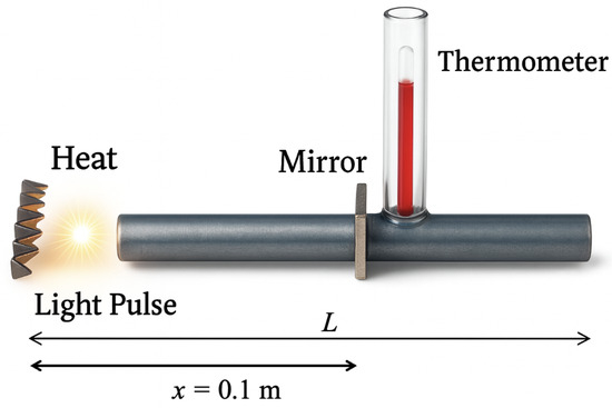
Figure 1.
Thought experiment relating causality and heat conduction.
How can we solve this inconsistency? Let us first express the energy in function of n and T and consider the total time derivative [4]:
where n is the particle number density. Here is where several undergraduate physics books neglect density variations, that is , transforming Equation (2) into
obtaining, using the Fourier constitutive equation (), Equation (1), the well-known heat equation. Further details regarding this derivation are included in Appendix A. The point is that in engineering applications, this approximation allows calculations with the necessary precision. However, in the relativistic regime, the difference is noticeable and it is important to ensure compliance with the principle of antecedence. If density variations are not neglected, a hyperbolic set of equations, instead of a parabolic single equation is obtained, predicting a finite propagation speed. This problem will be addressed in the next sections, using the whole set of equations for a relativistic fluid.
3. Kinetic Foundations and Transport Equations
For decades, relativistic kinetic theory has been successfully applied in the study of high temperature fluids [11]. Interest in relativistic transport theory has increased due to the detection of high-temperature plasmas generated in devices such as the Relativistic Heavy Ion Collider (RHIC). In this context, experiments involving collisions between heavy ions have been conducted, and electron-positron plasmas have been generated. In these scenarios, a fluid in the Euler regime (one in which viscosities and external forces are neglected) proves to be a good approximation for events involving collisions between gold ions [12]. Furthermore, the application of relativistic hydrodynamics in the field of astrophysics, and in particular in cosmology, remains of great interest [13]. Now then, the equations governing fluid dynamics can be established from different perspectives. The kinetic theory of gases, is the tool used in this research. It establishes its conclusions from first principles, without neglecting the physical meaning of quantities; it is based on microscopic theories of matter and the use of distribution functions. However, alternative approaches have been used to analyze thermodynamic systems. Examples of other methodologies are variational calculus and the phenomenological approach, which is based on empirical reasoning based on conservation laws. In this section, the kinetic theory of relativistic gases is revisited with the goal of clarifying and refining the causal structure of relativistic Euler fluids. This extended treatment corrects and enriches previous derivations, providing a more precise theoretical basis for the analysis of fluctuation dynamics within the Euler regime.
The starting point here is the relativistic Boltzmann equation for a simple fluid in the absence of external forces:
where c is the speed of light. In Equation (4), f is the distribution function in the phase space, is the collisional kernel, the three spatial components of the molecular velocity are given by and, as usual, . The relativistic generalization of Enskog’s transport equation can be casted in the form [1,11]:
The average of the collisional invariant is defined as
with [14].
In the Euler regime, all averages are calculated using the equilibrium () distribution function, valid for a non-degenerate gas [11]:
where is the relativistic parameter, k the Boltzmann constant, m the mass, and is the modified Bessel function of the second kind. When , the system is in a non-relativistic regime because the thermal energy of the particle is much lower than its rest energy. For , the system is said to be ultrarelativistic, where the rest energy of the particle is much lower than its thermal energy; it could be an electron gas, for example, whose mass is very small and has a very high temperature [15]. Figure 2a–c, where the relationships f vs. are shown, and denotes the speed in both the non-relativistic and relativistic cases, show both distributions for different values of z, showing how as this parameter increases, the difference between both distributions becomes significant. This illustrates why, in the relativistic case, instead of the Maxwell–Boltzmann distribution function, which accepts infinite molecular velocities, the Jüttner distribution function must be used.
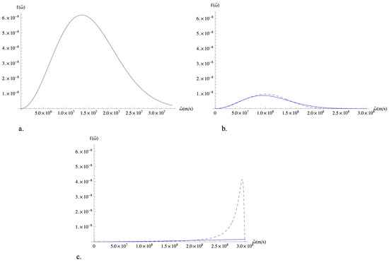
Figure 2.
Comparison of the non-relativistic Maxwell–Boltzmann distribution (solid line) and the relativistic Jüttner distribution (dashed line) for different values of z. Panels (a)–(c) show the comparison for , , and respectively.
Derivatives with respect to must be explicitly evaluated in Equation (7). After this operation, for the sake of simplicity, all calculations will be performed in the comoving frame of the fluid, where the observer is supposed to move with the average velocity of the fluid.
Now, the collisional invariants are (a constant), , and (the mechanical energy), where is the Lorentz factor. For , the continuity equation follows immediately
Substituting , the momentum balance equation is obtained:
The use of Equations (6) and (7) allows us to rewrite Equation (9) in terms of the local thermodynamic variables:
where the internal energy per particle reads [11]:
and the pressure satisfies the state equation
Finally, for , the resulting balance equation reads
or, in terms of the thermodynamic variables,
in Equation (14), we have defined . The set of Equations (8), (10), and (14) is highly nonlinear, and its full treatment is rather complex. For a system close to equilibrium, we linearize this set in order to perform a fluctuation analysis for the thermodynamical variables.
4. Linearized Equations and Causality Analysis
A system of differential equations as the one we deal with in the previous section (clearly not linear) can be treated, among other methods, by numerical techniques, qualitative theory or linearization. For the linearization procedure, we will allow the three thermodynamic functions (temperature T, density n, and velocity ) to fluctuate around a known average value. In order to proceed with the analysis of the Euler system, Equations (8), (10), and (14) close to equilibrium, we write any thermodynamical variable X into a constant average value and a space and time dependent fluctuation , so that
According to this definition, neglecting second order terms, the linearized continuity equation, obtained from (8) reads
Analogously, the linearized momentum balance for the longitudinal mode becomes
where we have defined . For the linearized energy balance equation, we obtain
Here, the heat capacity (per particle) is given by
Preserving the hyperbolic structure of the transport equations requires retaining velocity fluctuations. There is an illustrative analogy of this situation in electrodynamics, in the treatment of Maxwell equations (see Appendix B). Following these ideas, it became pertinent to revise the causality properties in this kind of systems, focusing on the possibility of generating a hyperbolic partial differential equation describing temperature fluctuations. One important aspect of the formalism shown above is the reference system. It has the physical capability to make the average speed equal to zero, but not the fluctuations itself.
To decouple the system and derive a partial differential equation for and , we begin by solving for on both sides of Equations (16) and (18). By equating the resulting expressions, we obtain the following useful relation:
and by integrating both sides of Equation (20), we obtain
where is a function that arises from integral calculus and depends only on . Now the derivative with respect to time is taking in both sides of Equation (16):
and the expression is substituted, taken from the momentum-balanced Equation (17):
In Appendix C, it is shown that so that density fluctuations satisfy a wave equation:
A similar calculation can be performed in order to find the wave equation for thermal fluctuations , which leads to
Thus, the propagation speed () of a thermal wave in a relativistic Euler fluid is
In the non-relativistic limit, the heat capacity per particle reduces to and the density , so that Equation (28) yields
which is the non-relativistic speed of sound, as expected. Also, the relativistic propagation speed Equation (28) can be rewritten in terms of z as
It is interesting to notice that some authors perform a similar analysis for neglecting temperature fluctuations, and only taking into account Equations (8) and (10), in order to establish a wave equation for density fluctuations [16]. In that case, it immediately finds out that the corresponding propagation speed is
In the same order of ideas, one can make a simple analysis neglecting the number density fluctuations and taking into account only Equations (10) and (18). In this case, the expression for temperature fluctuations speed propagation reads
Figure 3 shows a comparison of the characteristic speeds for increasing z.
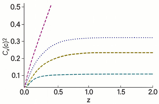
Figure 3.
Comparison of fluctuation propagation speeds for the full relativistic case (blue), non-relativistic case (purple), fluctuations neglecting thermal fluctuations (olive) and fluctuations neglecting number density fluctuations (green).
We have then calculated the characteristic speeds of the different fluctuations arising from hyperbolic equations.
5. Final Remarks
In this paper, an intuitive way to analyze causality has been presented in the context of thermal wave propagation. This approach focuses on two elements: working with the complete set of transport equations, which leads to a hyperbolic (not a parabolic) system and to the estimation of the characteristic propagation speeds.
It is shown that, in the Euler regime, there is no causality problem regarding thermodynamic fluctuations. The linearized transport equations become a hyperbolic system that, for further research, can be taken as a starting point as a simplified calculation and for validation of numerical work in the non-linear case.
The non-relativistic limit for the fluctuations’ speed has been recovered, as expected. It is important to remark that thermal fluctuations also satisfy a hyperbolic partial differential equation. In most textbooks, the establishment of the (parabolic) heat equation is based on an extension of Equation (14) including heat conduction, neglecting the velocity fluctuations. On the other hand, if the linearized equation of motion (17) is taken as the basis of the description of thermal fluctuations, then a causal equation is obtained for the non-dissipative fluid. Thus, for the dissipative case, it is suggested that the suitable generalization of the whole linearized system (8), (10) and (14) should be taken into account, emphasizing the role of Equation (10) while analyzing causal properties of the system. Neglecting velocity fluctuations clearly leads to causality problems. Moreover, taking is quite unrealistic, since when the fluid is at rest the mean velocity may be zero, but the fluctuations certainly do not vanish.
It can be noted, also, that density fluctuations (neglecting the thermal ones) and thermal fluctuations (neglecting the density ones) present different propagation speeds, satisfying the relation . The approximate Equations (31) and (32) may be useful in particular situations involving dissipative effects. In this case, it is complicated to uncouple the system of transport equations in the and t domain. Nevertheless, this can be achieved in the Fourier–Laplace space, where the Rayleigh–Brillouin spectrum can be established. Using this technique, the issue of causality can also be addressed obtaining very similar results as the ones included in this work [9]. At the Navier–Stokes level, a test was developed in [9] that allows for determining whether a set of linearized transport equations leads to a causal solution or not. When calculations are performed using the Eckart formalism, and with a large z, the Rayleigh peak invades the two Brillouin peaks, entering the forbidden region of the frequency cone. This indicates that the problem of non-causality arises due to the coupling of heat flux with acceleration. On the other hand, solutions are causal when using the constitutive equation for heat flux, which has been called the modified Eckart formalism [6]. Everything indicates that kinetic theory, particularly with this constitutive equation for heat flow, allows for a novel treatment, free of instabilities (at least in the generic sense, detected by Hiscock and Lindblom) and non-causal behavior.
Furthermore, it must be acknowledged that Linear Irreversible Thermodynamics is limited to operating in systems in equilibrium, or at least close to equilibrium, since there are various natural phenomena that develop out of equilibrium, such as viscoelastic media, polymeric fluids, and the formation of shock waves in matter, in which cases the linearized equations used in the analysis presented here do not adequately describe these dynamics. Despite this, the contribution of kinetic theory, even in the regime close to local equilibrium, is considered fundamental for numerical developments that allow us to address, albeit for the time being, the situations described that clearly develop outside of local equilibrium. This would allow an exploration of whether the causal structure is preserved or modified in such regimes.
Author Contributions
Conceptualization: D.B.-B.; Formal analysis: A.S.-V. and D.B.-B.; Investigation: A.S.-V. and D.B.-B.; Methodology: D.B.-B. and H.E.C.-O.; Writing (original and review): D.B.-B. and H.E.C.-O. A.S.-V. passed away prior to the publication of this manuscript. All authors have read and agreed to the published version of the manuscript.
Funding
No financial support was provided for this paper.
Data Availability Statement
No underlying data were collected or produced in this study.
Conflicts of Interest
The authors declare no conflicts of interest.
Appendix A. About the Parabolicity of the Heat Equation
In the previous section, it was shown that Equations (8), (10), and (14) are nonlinear and the same set of equations is then linearized (for a system close to equilibrium) and a hyperbolic transport equations raised. Taking the same three equations and including a heat conduction term, we have
Making the differentiation for the energy term :
We obtain
The heat flux is proportional to
which is a parabolic equation. As stated before, parabolicity arises when is neglected in Equation (A3), this is not so at the level of fluctuations.
Appendix B. The Electromagnetic Field Case
In electromagnetic fields, a similar situation is present. No one would question if electromagnetic waves travel at the speed of light or not. The calculation which follows show the assumptions underlying this important result.
Let us begin with the set of Maxwell equations, which form the basis of all classical electro-magnetic phenomena [17]:
Making the electric density and the electric flux zero and using Equation (A10), we obtain
or, with the general form:
the wave equation; consequently, electrical phenomena travel like a wave with the speed of light (c). An analog expression is recovered for the magnetic case. What must be emphasized here is that if the time derivatives are neglected, a parabolic, instead of a hyperbolic equation is obtained, meaning that electromagnetic fields would propagate instantaneously (Laplace equation).
Appendix C. Proof of ∇2R0 = 0
In this appendix, it is shown that the Laplacian of function which appears in Equations (24) and (25) has a value of zero, which implies that the density fluctuations () and the temperature ones () satisfy a wave equation. Let us begin with Equation (25) re-written as follows:
and is substituted from Equation (21):
from which
and after a rearrangement of terms,
The two first terms on Equation (A14) correspond to the left hand term on Equation (25), for what is obtained as follows:
now all the terms of the left-hand side of the equation are transferred:
and after a rearrangement of terms,
from which it is finally obtained that
which is the objective of this demonstration.
References
- Sandoval-Villalbazo, A.; Garcia-Colin, L.S. The relativistic kinetic formalism revisited. Phys. A Stat. Mech. Its Appl. 2000, 278, 428–439. [Google Scholar] [CrossRef]
- Eckart, C. The Thermodynamics of Irreversible Processes. III. Relativistic Theory of the Simple Fluid. Phys. Rev. 1940, 58, 267. [Google Scholar] [CrossRef]
- Landau, L.; Lifshitz, E.M. Fluid Mechanics; Addison Wesley: Boston, MA, USA, 1958. [Google Scholar]
- de Groot, S.R.; van Leeuwen, W.A.; van der Weert, C. Relativistic Kinetic Theory; North Holland Publ. Co.: Amsterdam, The Netherlands, 1980. [Google Scholar]
- Denicol, G.S.; Koide, T.; Mota, P. Stability and causality in relativistic dissipative hydrodynamics. J. Phys. G 2008, 35, 115102. [Google Scholar] [CrossRef]
- Garcia-Perciante, A.L.; Garcia-Colin, L.S.; Sandoval-Villalbazo, A. On the nature of the so-called generic instabilities in dissipative relativistic hydrodynamics. Gen. Rel. Grav. 2009, 41, 1645–1654. [Google Scholar] [CrossRef][Green Version]
- Hiscock, W.A.; Lindblom, L. Generic instabilities in first-order dissipative relativistic. Phys. Rev. D 1985, 31, 725. [Google Scholar] [CrossRef] [PubMed]
- Israel, W. Transient relativistic thermodynamics and kinetic theory. Ann. Phys. 1976, 100, 310. [Google Scholar] [CrossRef]
- Brun-Battistini, D.; Sandoval-Villalbazo, A. Light Cone analysis of relativistic first-order in the gradients hydrodynamics. In Proceedings of the IV Mexican Meeting on Mathematical and Experimental Physics, Mexico City, Mexico, 19 July 2010. [Google Scholar] [CrossRef]
- Borrelli, R.; Coleman, C. Differential Equations: A Modeling Approach; Prentice Hall: Hoboken, NJ, USA, 1987. [Google Scholar]
- Cercignani, C.; Medeiros Kremer, G. The Relativistic Boltzmann Equation: Theory and Applications; Birkhuser: Berlin, Germany, 2002. [Google Scholar]
- Kolb, P.F.; Heinz, U. Hydrodynamic description of ultrarelativistic heavyion collisions. In Quark Gluon Plasma 3; Hwa, R.C., Wang, X.-N., Eds.; World Scientific: Singapore, 2004; pp. 634–714. [Google Scholar]
- Weinberg, S. Gravitation and Cosmology: Principles and Applications of the General Theory of Relativity; John Wiley & Sons: Hoboken, NJ, USA, 1972. [Google Scholar]
- Liboff, R.L.; Liboff, R.C. Kinetic Theory: Classical, Quantum and Relativistic Descriptions; Springer: Berlin, Germany, 2003. [Google Scholar]
- Chacón-Acosta, G. Cien años de la función de distribución de Jüttner para el gas relativista. Rev. Mex. Fís. 2012, 58, 117–126. [Google Scholar]
- Kolb, E.W.; Turner, M.S. The Early Universe; Addison-Wesley: Reading, MA, USA, 1990. [Google Scholar]
- Jackson, J.D. Classical Electrodynamics; Wiley: New York, NY, USA, 1999. [Google Scholar]
Disclaimer/Publisher’s Note: The statements, opinions and data contained in all publications are solely those of the individual author(s) and contributor(s) and not of MDPI and/or the editor(s). MDPI and/or the editor(s) disclaim responsibility for any injury to people or property resulting from any ideas, methods, instructions or products referred to in the content. |
© 2025 by the authors. Licensee MDPI, Basel, Switzerland. This article is an open access article distributed under the terms and conditions of the Creative Commons Attribution (CC BY) license (https://creativecommons.org/licenses/by/4.0/).