Abstract
In this paper, we develop a geometric formulation of datasets. The key novel idea is to formulate a dataset to be a fuzzy topological measure space as a global object and equip the space with an atlas of local charts using graphs of fuzzy linear logical functions. We call such a space a logifold. In applications, the charts are constructed by machine learning with neural network models. We implement the logifold formulation to find fuzzy domains of a dataset and to improve accuracy in data classification problems.
Keywords:
logifold; dataset; neural network; measure theory; fuzzy space; data classification; machine learning MSC:
46S40; 14P10; 68T07; 53Z50
1. Introduction
In geometry and topology, the manifold approach dates back to Riemann using open subsets in as local models to build a space. Such a local-to-global principle is central to geometry and has achieved extremely exciting breakthroughs in modeling spacetime by Einstein’s theory of relativity.
In recent years, the rapid development of data science brings immense interest to datasets that are ‘wilder’ than typical spaces that are well-studied in geometry and topology. Taming the wild is a central theme in the development of mathematics. Advances in computational tools have helped to expand the realm of mathematics in history. For instance, it took many years in human history to recognize the irrational number and approximate it by rational numbers. In this regard, we consider machine learning by neural network models as a modern tool to find expressions of a ‘wild space’ (for instance a dataset in real life) as a union (limit) of fuzzy geometric spaces expressed by finite formulae.
The mathematical background of this paper lies in manifold, probability, and measure theory. Only basic mathematical knowledge in these two subjects is necessary. For instance, the textbooks [1,2] provide excellent introduction to measure theory and manifold theory, respectively.
Let X be a topological space, the corresponding Borel -algebra, and a measure on . We understand a dataset, for instance, the collection of all labeled appearances of cats and dogs, as a fuzzy topological measure space in nature. In the example of cats and dogs, topology concerns about the nearby appearances of the objects; measure concerns about how typical each appearance is; and fuzziness comes from how likely the objects belonging to cats, dogs, or neither.
To work with such a complicated space, we would like to have local charts that admit finite mathematical expressions and have logical interpretations, playing the role of local coordinate systems for a measure space. In our definition, a local chart is required to have a positive measure. Moreover, to avoid triviality and requiring too many charts to cover the whole space, we may further fix and require that . Such a condition disallows U to be too simple, such as a tiny ball around a point in a dataset. This resembles the Zariski-open condition in algebraic geometry.
In place of open subsets of , we formulate ‘local charts’ that are closely related to neural network models and have logic gate interpretations. Neural network models provide a surprisingly successful tool for finding mathematical expressions that approximate a dataset. Non-differentiable or even discontinuous functions analogous to logic gate operations are frequently used in network models. It provides an important class of non-smooth and even discontinuous functions to study a space.
We take classification problems as the main motivation in this paper. For this, we consider the graph of a function , where D is a measurable subset in (with the standard Lebesgue measure) and T is a finite set (with the discrete topology). The graph is equipped with the push-forward measure by .
We use the graphs of linear logical functions explained below as local models. A chart is of the form , where is a measurable subset which satisfies , and is a measure-preserving homeomorphism. We define a linear logifold to be a pair , where is a collection of charts such that . In applications, the condition makes sure that the logifold covers almost every element (in the measure-theoretical sense) in the dataset. Figure 1 provides a simple example for a logifold.
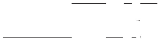
Figure 1.
An example of a logifold. The graph jumps over values 0 and 1 infinitely in left-approaching to the point marked by a star (and the length of each interval is halved). This is covered by infinitely many charts of linear logical functions, each of which has only finitely many jumps. Moreover, the base is a measurable subset of (which is hard to depict and not shown in the picture).
In the example of cats and dogs, is a representing sample collection of appearances of cats and dogs. We take 2D images with n number of pixels for these appearances and get a function where is the collection of the labels and is the collection of pictures. The image is given by the graph of a function , which tells whether each picture shows a cat or a dog.
The definition of linear logical functions is motivated from neural network models and has a logic gate interpretation. A network model consists of a directed graph, whose arrows are equipped with linear functions and vertices are equipped with non-linear functions, which are typically ReLu or sigmoid functions in middle layers and are sigmoid or softmax functions in the last layer. The review paper [3] provides an excellent overview of deep learning models. Note that sigmoid and softmax functions are smoothings of the discrete-valued step function and the index-max function, respectively. Such smoothings are useful to describe the fuzziness of data.
From this perspective, step and index-max functions are the non-fuzzy (or called classical) limit of sigmoid and softmax functions, respectively. We will take such a limit first, and come back to fuzziness in a later stage. This means we replace all sigmoid and softmax functions in a neural network model by step and index-max functions. We will show that such a neural network is equivalent to a linear logical graph as follows: at each node of the directed graph, there is a system of N linear inequalities (on the input Euclidean domain ) that produces possible Boolean outcomes for an input element, which determine the next node that this element will be passed to. We call the resulting function a linear logical function.
From the perspective of functional analysis, the functions under consideration have targets being finite sets or simplices, which are not vector spaces. Thus, the set of functions is NOT a vector space. This is the main difference from the typical setting of Fourier analysis. We discuss more about this aspect using semiring structures in Section 2.5.
We prove that linear logical functions can approximate any given measurable function , where D is a measurable subset of with . This provides a theoretical basis of using these functions in modeling.
Theorem 1
(Universal approximation theorem by linear logical functions). Let be a measurable function whose domain is of finite Lebesgue measure, and suppose that its target set T is finite. For any , there exists a linear logical function L and a measurable set of the Lebesgue measure less than ϵ such that .
By taking the limit , the above theorem finds a linear logifold structure on the graph of a measurable function. In reality, reflects the error of a network in modeling a dataset.
It turns out that for , linear logical functions (where T is identified with a finite subset of ) are equivalent to semilinear functions , whose graphs are semilinear sets defined by linear equations and inequalities [4]. Semilinear sets provide the simplest class of definable sets of so-called o-minimal structures, which are closely related to model theory in mathematical logic. O-minimal structures made an axiomatic development of Grothendieck’s idea of finding tame spaces that exclude wild topology. On the one hand, definable sets have a finite expression which is crucial to the predictive power and interpretability in applications. On the other hand, our setup using measurable sets provides a larger flexibility for modeling data.
Compared to more traditional approximation methods such as Fourier series, there are reasons why linear logical functions are preferred in many situations for data. When the problem is discrete in nature (for instance the target set T is finite), it is simple and natural to take the most basic kinds of discrete-valued functions as building blocks, namely step functions formed by linear inequalities. These basic functions are composed to form networks which are supported by current computational technology. Moreover, such discrete-valued functions have fuzzy and quantum deformations which have rich meanings in mathematics and physics.
Now let us address fuzziness, another important feature of a dataset besides discontinuities. In practice, there is always an ambiguity in determining whether a point belongs to a dataset. This is described as a fuzzy space , where X a topological measure space and is a continuous measurable function that encodes the probability of whether a given point of X belongs to the fuzzy space under consideration. Here, we require on purpose, and while points of zero probability of belonging may be adjoined to X to that the union gets simplified (for instance, X may be embedded into , where points in have zero probability of belonging), they are auxiliary and have no intrinsic meaning.
Let us illustrate by the above-mentioned example of cats and dogs. The fuzzy topological measure space X consists of all possible labeled appearances of cats and dogs. The function value expresses the probability of x belonging to the dataset, in other words, how likely the label for the appearance is correct.
To be useful, we need a finite mathematical expression (or approximation) for . This is where neural network models enter into the description. A neural network model for a classification problem that has the softmax function in the last layer gives a function , where S is the standard simplex . This gives a fuzzy space
where and . As we have explained above, in the non-fuzzy limit, sigmoid and softmax functions are replaced by their classical counterparts of step and index-max functions, respectively, and we obtain and the subset as the classical limit. Figure 2 shows a very simple example of a fuzzy space and its classical and quantum analogs.

Figure 2.
The left hand side shows a simple example of a logifold. It is the graph of the step function . The figure in the middle shows a fuzzy deformation of it, which is a fuzzy subset in . The right hand side shows the graph of the probability distribution of a quantum observation, which consists of the maps and from the state space to .
However, the ambient space is not intrinsic; for instance, in the context of images, the dimension n gets bigger if we take images with higher resolutions, even though the objects under concern remain the same. Thus, like in manifold theory, the target space is taken to be a topological space rather than , and our theory takes a topological measure space X in place of (or ). (for various possible n) is taken as an auxiliary ambient space that contains (fuzzy) measurable subsets that serve as charts to describe a dataset .
Generally, we formulate fuzzy linear logical functions (Definition 2) and fuzzy linear logifolds (Definition 9). A fuzzy logical graph is a directed graph G whose each vertex of G is equipped with a state space, and each arrow is equipped with a continuous map between the state spaces. The walk on the graph (determined by inequalities) depends on the fuzzy propagation of the internal state spaces.
Our logifold formulation of a dataset can be understood as a geometric theory for ensemble learning and the method of Mixture of Experts. Ensemble learning utilizes multiple trained models to make a decision or prediction, see, for instance [5,6,7]. Ensemble machine learning achieves improvement in classification problems, see, for instance [8,9]. In the method of Mixture of Experts (see, for instance [10,11]), several expert models are employed, and there is also a gating function . The final outcome is given by the total . This idea of using ‘experts’ to describe a dataset is similar to the formulation of a fuzzy logifold. On the other hand, motivated by manifold theory, we formulate universal mathematical structures that are common to datasets, namely the global intrinsic structure of a fuzzy topological measure space, and local logical structures among data points expressed by graphs of fuzzy logical functions.
The research design of this paper is characterized by its dual approach, outlined as follows: it involves rigorous mathematical constructions and formalization of logifolds and their properties, complemented by the design of algorithms, empirical validation through experiments that demonstrate their practical advantages in enhancing prediction accuracy for ensemble machine learning. This dual approach ensures both the theoretical soundness and practical utility of the proposed framework.
For readers who are more computationally oriented, they can first directly go to Section 4, where we describe the implementation of the logifold theory in algorithms. The key new ingredient in our implementation is the fuzzy domain of each model. A trained model typically does not have a perfect accuracy rate and performs well only on a subset of data points, or for a subset of target classes. A major step here is to find and record the domain of each model where it works well. Leveraging certainty scores derived from the softmax outputs of classifiers, a model’s prediction is only used in the implemented logifold structure if its certainty exceeds a predefined threshold, allowing for a refined voting system (Section 4.5).
Two experiments were conducted for logifold and they were published in our paper [12] using the refined voting system on the following well-known benchmark datasets: CIFAR10 [13], MNIST [14], and Fashion MNIST [15]. We summarize the experimental results in Section 5.
Organization
The structure of this paper is as follows. First, we formulate fuzzy linear logical functions in Section 2. Next, we establish relations with semilinear functions in Section 3.1, prove the universal approximation theorem for linear logical functions in Section 3.2, and define fuzzy linear logifolds in Section 3.3. We provide a detailed description of the algorithmic implementation of logifolds in Section 4.
2. Linear Logical Functions and Their Fuzzy Analogs
Given a subset of , one would like to describe it as the zero locus, the image, or the graph of a function in a certain type. In analysis, we typically think of continuous/smooth/analytic functions. However, when the domain is not open, smoothness may not be the most relevant condition.
The success of network models has taught us a new kind of function that is surprisingly powerful in describing datasets. Here, we formulate them using directed graphs and call them linear logical functions. The functions offer three distinctive advantages. First, they have the advantage of being logically interpretable in theory. Second, they are close analogues of quantum processes. Namely, they are made up of linear functions and certain non-linear activation functions, which are analogous to unitary evolution and quantum measurements. Finally, it is natural to add fuzziness to these functions and hence they are better adapted to describe statistical data.
2.1. Linear Logical Functions and Their Graphs
We consider functions for and a finite set T constructed from a graph as follows. Let G be a finite directed graph that has no oriented cycle and has exactly one source vertex which has no incoming arrow and target vertices. Each vertex that has more than one outgoing arrows is equipped with an affine linear function on , where the outgoing arrows at this vertex are one-to-one corresponding to the chambers in subdivided by the hyperplanes . Explicitly, let , and consider
If is non-empty, we call a chamber associated with .
Definition 1.
A linear logical function is a function made in the following way from , where G is a finite directed graph that has no oriented cycle and has exactly one source vertex and target vertices,
are affine linear functions whose chambers in D are one-to-one corresponding to the outgoing arrows of v. is called a linear logical graph.
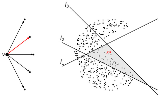
Given , we get a path from the source vertex to one of the target vertices in G as follows. We start with the source vertex. At a vertex v, if there is only one outgoing arrow, we simply follow that arrow to reach the next vertex. If there are more than one outgoing arrows, we consider the chambers made by the affine linear function associated with the vertex v, and pick the outgoing arrow that corresponds to the chamber that x lies in. See Figure 3. Since the graph is finite and has no oriented cycle, we will stop at a target vertex, which is associated with an element . This defines the function by setting .
Figure 3.
The left side shows a partial directed graph at vertex v, with five outgoing arrows. On the right, chambers are formed in by the affine maps defined on . A point x is marked in the chamber defined by . One of the arrows corresponding to the shaded chamber containing x is highlighted in the left diagram.
Proposition 1.
Consider a feed-forward network model whose activation function at each hidden layer is the step function and that at the last layer is the index-max function. The function is of the form
where are affine linear functions with , are the entrywise step functions and σ is the index-max function. We make the generic assumption that the hyperplanes defined by for do not contain . Then this is a linear logical function with target (on any , where is the domain of ).
Proof.
The linear logical graph is constructed as follows. The source vertex is equipped with the affine linear function . Then we make N number of outgoing arrows of (and corresponding vertices), where N is the number of chambers of , which are one-to-one corresponding to the possible outcomes of (which form a finite subset of ). Then we consider restricted to this finite set, which also has a finite number of possible outcomes. This produces exactly one outgoing arrow for each of the vertices in the first layer. We proceed inductively. The last layer is similar and has possible outcomes. Thus, we obtain as claimed, where L consists of only one affine linear function over the source vertex. □
Figure 4 depicts the logical graph in the above proposition.
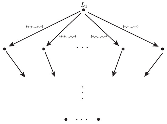
Figure 4.
A linear logical graph for a feed-forward network whose activation function at each hidden layer is the step function and that at the last layer is the index-max function.
Proposition 2.
Consider a feed-forward network model whose activation function at each hidden layer is the ReLu function and that at the last layer is the index-max function. The function takes the form
where are affine linear functions with , are the entrywise ReLu functions, and σ is the index-max function. This is a linear logical function.
Proof.
We construct a linear logical graph , which produces this function. The first step is similar to the proof of the above proposition. Namely, the source vertex is equipped with the affine linear function . Next, we make N number of outgoing arrows of (and corresponding vertices), where N is the number of chambers of , which are one-to-one corresponding to the possible outcomes of the sign vector of (which form a finite subset of ). Now we consider the next linear function . For each of these vertices in the first layer, we consider restricted to the corresponding chamber, which is a linear function on the original domain , and we equip this function to the vertex. Again, we make a number of outgoing arrows that correspond to the chambers in made by this linear function. We proceed inductively, and get to the layer of vertices that correspond to the chambers of . Write , and consider . At each of these vertices,
restricted on the corresponding chamber is a linear function on the original domain , and we equip this function to the vertex and make outgoing arrows corresponding to the chambers of the function. In each chamber, the index i that maximizes is determined, and we make one outgoing arrow from the corresponding vertex to the target vertex . □
By the above propositions, ReLu/sigmoid-based feed forward network functions are linear logical functions. Thus, the above linear logical functions have the same computational complexity as the corresponding ReLu/sigmoid-based functions. Figure 5 depicts the logical graph in the above proposition.
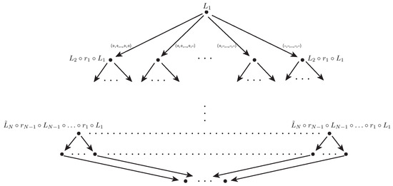
Figure 5.
The linear logical graph for a feed-forward network whose activation function at each hidden layer is the ReLu function and that at the last layer is the index-max function.
In classification problems, T is the set of labels for elements in D, and the data determine a subset in as a graph of a function. The deep learning of network models provides a way to approximate the subset as the graph of a linear logical function . Theoretically, this gives an interpretation of the dataset; namely, the linear logical graph gives a logical way to deduce the labels based on linear conditional statements on D.
The following lemma concerns the monoidal structure on the set of linear logical functions on D.
Lemma 1.
Let be linear logical functions for , where . Then
is also a linear logical function.
Proof.
We construct a linear logical graph out of for as follows. First, take the graph . For each target vertex of , we equip it with the linear function at the source vertex of and attach to it the graph . The target vertices of the resulting graph are labeled by . Similarly, each target vertex of this graph is equipped with the linear function at the source vertex of and attached with graph . Inductively, we obtain the required graph, whose target vertices are labeled by . By this construction, the corresponding function is . □
admits the following algebraic expression in the form of a sum over paths which has an important interpretation in physics. The proof is straightforward and is omitted. A path in a directed graph is a finite sequence of composable arrows. The set of all linear combinations of paths and the trivial paths at vertices form an algebra by concatenation of paths.
Proposition 3.
Given a linear logical graph ,
where the sum is over all possible paths γ in G from the source vertex to one of the target vertices; denotes the target vertex that γ heads to for ,
where if x lies in the chamber corresponding to the arrow a; otherwise, it is 0. In the above sum, exactly one of the terms is non-zero.
2.2. Zero Locus
Alternatively, we can formulate the graphs as zero loci of linear logical functions targeted at the field with two elements as follows. Such a formulation has the advantage of making the framework of algebraic geometry available in this setting.
Proposition 4.
For each linear logical function , there exists a linear logical function whose zero locus in equals .
Proof.
Given a linear logical function , we construct another linear logical function as follows. Without loss of generality, let , so that is embedded as a subset of . Any linear function on is pulled back as a linear function on by the standard projection that forgets the last component. Then is lifted as a linear logical function .
Consider the corresponding graph . For the k-th target vertex of (that corresponds to ), we equip it with the linear function
where y is the last coordinate of . This linear function produces three chambers in . Correspondingly, we make three outgoing arrows of the vertex. Finally, the outcome vertex that corresponds to is connected to the vertex ; the other two outcome vertices are connected to the vertex . We obtain a linear logical graph and the corresponding function .
By construction, for if and only if . Thus, the zero locus of is the graph of . □
The set of functions (with a fixed domain) valued in forms a unital commutative and associative algebra over , which is known as a Boolean algebra.
Proposition 5.
The subset of linear logical functions forms a Boolean ring (for a fixed ).
Proof.
We need to show that the subset is closed under addition and multiplication induced from the corresponding operations of .
Let and be linear logical functions . By Lemma 1, is a linear logical function. Consider the corresponding logical graph. The target vertices are labeled by . We connect each of them to the vertex by an arrow. This gives a linear logical graph whose corresponding function is . We obtain in a similar way. □
In this algebro-geometric formulation, the zero locus of corresponds to the ideal .
2.3. Parameterization
The graph of a linear logical function can also be put in parametric form. For the moment, we assume the domain D is finite. First, we need the following lemma.
Lemma 2.
Assume is finite. Then the identity function is a linear logical function.
Proof.
Since D is finite, there exists a linear function such that each chamber of l contains at most one point of D. Then we construct the linear logical graph G as follows. The source vertex is equipped with the linear function l and outgoing arrows corresponding to the chambers of l. Elements of D are identified as the target vertices of these arrows which correspond to chambers that contain them. The corresponding function equals . □
Proposition 6.
Given a linear logical function with finite , there exists an injective linear logical function whose image equals .
Proof.
By Lemmas 1 and 2, is a linear logical function. By definition, its image equals . □
2.4. Fuzzy Linear Logical Functions
Another important feature of a dataset is its fuzziness. Below, we formulate the notion of a fuzzy linear logical function and consider its graph. Basic notions of fuzzy logic can be found in textbooks such as [16]. There are many developed applications of fuzzy logic such as modeling, control, pattern recognition and networks, see, for instance [17,18,19,20,21].
Definition 2.
Let G be a finite directed graph that has no oriented cycle and has exactly one source vertex and target vertices as in Definition 1. Each vertex v of G is equipped with a product of standard simplices
for some integers , . is called the internal state space of the vertex v. Let D be a subset of the internal state space of the source vertex of G. Each vertex v that has more than one outgoing arrow is equipped with an affine linear function
for some , and we require that the collection of non-empty intersections of the chambers of with the product simplex are one-to-one corresponding to the outgoing arrows of v. Let L denote the collection of these affine linear functions . Moreover, each arrow a is equipped with a continuous function
where denote the source and target vertices, respectively.
We call a fuzzy linear logical graph. Let denote the disjoint union . determines a function
as follows. Given , it is an element of the internal state space of the source vertex v. Moreover, it lies in a unique chamber of the affine linear function at the source vertex v. Let be the head vertex of the outgoing arrow a corresponding to this chamber. We have the element . By repeating this process, we obtain a path from the source vertex to one of the target vertices , and also an element in the internal state space that we define as . The resulting function is called a fuzzy linear logical function.
In the above definition, a standard choice of a continuous map between product simplices
is using the softmax function :
where are affine linear functions. is defined by
This is the sigmoid function when .
Remark 1.
We can regard the definition of a fuzzy linear function as a generalization of the linear logical function in Definition 1. Note that the linear functions in L in the above definition have domain to be the internal state spaces over the corresponding vertices v. In comparison, the linear functions in L in Definition 1 have domain as the input space . A linear logical graph in Definition 1 has no internal state space except the at the input vertex.
To relate the two notions given by the above definition and Definition 1, we can set as the same for all vertices v except the target vertices , which are equipped with the zero-dimensional simplex (a point), and we set as the identity maps for all arrows a that are not targeted at any of . Then reduces back to a linear logical function in Definition 1.
Remark 2.
We call the corners of the convex set state vertices, which take the form for a multi-index , where is the standard basis. We have a bigger graph by replacing each vertex v of G by the collection of state vertices over v and each arrow of G by the collection of all possible arrows from source state vertices to target state vertices. Then the vertices of G are interpreted as ‘layers’ or ‘clusters’ of vertices of . The input state , the arrow linear functions L, and the maps between state spaces p determine the probability of getting to each target state vertex of from the source vertex.
In this interpretation, we take the target set to be the disjoint union of corners of at the target vertices as follows:
which is a finite set. The function determines the probability of the outcome for each input state as follows. Let for some . Then the probability of being in is zero for . Writing for , the probability of the output to be for is given by .
Proposition 7.
Consider the function
given by a feed-forward network model whose activation function at each hidden layer is the sigmoid function (denoted by ), and that at the last layer it is the softmax function . f is a fuzzy linear logical function.
Proof.
We set as follows. G is the graph that has vertices with arrows from to for . L is just an empty set. for , where is the dimension of the domain of . The one-dimensional simplex is identified with the interval . , where is the dimension of the target of . Then
Then . □
Proposition 8.
Consider the function
given by a feed-forward network model whose activation function at each hidden layer is the ReLu function (denoted by ), and that at the last layer it is the softmax function . Here, each denotes an affine linear function. The function f is a fuzzy linear logical function.
Proof.
We need to construct a fuzzy linear logical graph such that . We take G to be the logical graph constructed in Example 2 (Figure 5) with the last two layers of vertices replaced by a single target vertex t. Each vertex that points to the last vertex t and t itself only has zero or one outgoing arrow and hence is not equipped with a linear function. Other vertices are equipped with linear functions on the input space as in Example 2. We take the internal state space to be the n-dimensional cube , where n is the input dimension at every vertex v except at the target vertex, whose internal state space is defined to be the simplex , where d is the target dimension of f. The function in Definition 2 is defined to be the identity function on the internal state space for every arrow a except for the arrows that point to t. Now, we need to define for the arrows that point to t. Let be the source vertices of these arrows. The input space is subdivided into chambers . Moreover, is a piecewise-linear function, whose restrictions on each of these chambers is linear and extend to a linear function l on . Then for the corresponding arrow a is defined to be . By this construction, we have . □
As in Proposition 3, can be expressed in the form of the sum over paths.
Proposition 9.
Given a fuzzy linear logical graph ,
where the sum is over all possible paths γ in G from the source vertex to one of the target vertices; for , ;
where if lies in the chamber corresponding to the arrow a or is 0 otherwise. In the above sum, exactly one of the terms is non-zero.
2.5. The Semiring of Fuzzy Linear Logical Functions
Since the target space is not a vector space, the set of functions does not form a vector space. This makes a main difference from usual approximation theory (such as Fourier analysis or Taylor series) where the function space is flat as the target is a vector space (typically ). For a fuzzy logic target (the product simplex in our case), the ‘function space’ forms a semiring. Due to this difference, we shall work out some well-known results in functional analysis in the semiring context below.
Recall that a semi-group is a set equipped with a binary operation that is associative; a monoid is a semi-group with an identity element. A semiring is a set equipped with two binary operations addition and multiplication which satisfy the ring axioms except for the existence of additive inverses. In particular, a semiring is a semi-group under addition and a semi-group under multiplication, and the two operations are compatible in the sense that multiplication distributes over addition. A semiring without a unit is a semiring that does not have a multiplicative identity.
Example 1
(Viterbi semiring). Let be the unit interval with the usual multiplication and addition defined as taking maximum. The additive identity is 0 and the multiplicative identity is 1. Then is a semiring. This is known as the Viterbi semiring that appears in probabilistic parsing.
The subset of two elements is a sub-semiring known as the Boolean semiring. Addition (taking maximum) and multiplication are identified as the logical operations OR and AND, respectively.
In this subsection, we focus on the case that the target space is a product of intervals .
Lemma 3.
The set of functions from a set D to (or ) has a semiring structure.
Proof.
For the semiring structure on (or ), we simply take entrywise addition and multiplication, where addition is defined as taking maximum and multiplication is the usual one. The additive identity is the origin and the multiplicative identity is . The set of functions to (or ) has a semiring structure by taking maximum and multiplication of function values. The additive identity is the zero function that takes all domain points to . □
Remark 3.
If we take a disjoint union of product simplices in place of , we still have a semi-group structure by entriwise multiplication. However, since taking the entriwise maximum does not preserve the inequality for a simplex, this destroys the semiring structure. This is why we restrict ourselves to in this section.
Theorem 2.
Fix D as a subset of a product simplex, and fix the target product of intervals . The set of fuzzy linear logical functions is a sub-semiring of the semiring of functions .
Similarly, the set of linear logical functions is a sub-semiring of the semiring of functions .
Proof.
Given two linear logical functions and with the same domain and target , we need to show that their sum (in the sense of entriwise maximum) and product are also linear logical functions. We construct a directed graph G with one source vertex and one target vertex by merging the target vertex of with the source vertex of as a single vertex, and then we add one outgoing arrow to the final vertex of to another vertex, which is the target of G.
Now for the internal state spaces, over those vertices v of G that belong to , we take ; over those v that belong to , we take . Note that the vertex that comes from merging of the target vertex of and the source vertex of is equipped with the internal state space ; the vertex that corresponds to the final vertex of is . The last vertex is equipped with the space .
The arrow maps are defined as follows. For arrows a that come from , we take the function . For arrows a that come from , we take the function . By this construction for an input , the value becomes at the vertex corresponding to the final vertex of . The last arrow is then equipped with the continuous function given by the entriwise maximum (or entriwise product). Thus, gives the function , which is the sum (or the product) of and .
The proof for the case of linear logical functions is similar and hence omitted. □
is equipped with the standard Euclidean metric . Moreover, the domain D is equipped with the Lebesgue measure . We consider the set of measurable functions .
Lemma 4.
The set of measurable functions form a sub-semiring.
Proof.
If are measurable functions, then is also measurable. Taking entriwise maximum and multiplication are continuous functions . Thus, the compositions, which give the sum and product of f and g, are also measurable functions. Furthermore, the zero function is measurable. Thus, the set of measurable functions forms a sum semiring. □
We define
To make this a distance function such that implies , we need to quotient out the functions whose support has measure zero.
Proposition 10.
The subset of measurable functions whose support has measure zero forms an ideal of the semiring of measurable functions . The above function d gives a metric on the corresponding quotient semiring, denoted by .
Proof.
The support of the sum is the union of the supports of f and g. The support of the product is the intersection of the supports of f and g. Thus, if the supports of f and g have measure zero, then so does the support of . Furthermore, if f has the support of measure zero, has the support of measure zero (with no condition on g). This shows that the subset of measurable functions with the support of measure zero forms an ideal.
d is well-defined on the quotient semiring because if f and g are in the same equivalent class, that is for some measurable functions whose support have measure zero, then for some set A of measure zero. Thus, for any other function h,
Now, consider any two elements in the quotient semiring. It is obvious that from the definition of d. Furthermore, the following triangle inequality holds:
Finally, suppose . This means that . Since the integrand is non-negative, we have for almost every . Thus, away from a measure zero subset . Since and (where denotes the characteristic function of the set A which takes value 1 on A and 0 otherwise), we have
□
Proposition 11.
is a topological semiring (under the topology induced from the metric d).
Proof.
We need to show that the addition and multiplication operations
is continuous. First, consider
This is continuous, as follows: for , consider with and . Then
by taking . Now, the function is Lipschitz continuous with Lipschitz constant 1. Entriwise multiplication is also Lipschitz continuous since the product is compact. Denote either one of these two functions by , and let K be the Lipschitz constant. As above, we have chosen suitable to control and such that
Then
□
2.6. Graph of Fuzzy Linear Logical Function as a Fuzzy Subset
A fuzzy subset of a topological measure space X is a continuous measurable function . This generalizes the characteristic function of a subset. The interval can be equipped with the semiring structure whose addition and multiplication are taking maximum and minimum, respectively. This induces a semiring structure on the collection of fuzzy subsets that plays the role of union and intersection operations.
The graph of a function
where are products of simplices as in Definition 2, is defined to be the fuzzy subset in , where T is defined by Equation (1), given by the probability at every determined by f in Remark 2.
The following is a fuzzy analog of Proposition 4.
Proposition 12.
Let be a fuzzy linear logical function. Let be the characteristic function of its graph where T is defined by (1). Then is also a fuzzy linear logical function.
Proof.
Similar to the proof of Proposition 4, we embed the finite set T as the subset . The affine linear functions on in the collection L are pulled back as affine linear functions on . Similarly for the input vertex , we replace the product simplex by (where the interval is identified with ); for the arrows a tailing at , are pulled back to be functions . Then, we obtain on G.
For each of the target vertices of G, we equip it with the linear function
where y is the last coordinate of the domain . It divides into chambers that contain for some . Correspondingly, we make outgoing arrows of the vertex . The new vertices are equipped with the internal state space , and the new arrows are equipped with the identity function . Then we get additional vertices, where K is the number of target vertices of G. Let us label these vertices as for and . Each of these vertices are connected to the new output vertex by a new arrow. The new output vertex is equipped with the internal state space . The arrow from to the output vertex is equipped with the following function . If , then we set . Otherwise, for and , , where are the coordinates of . This gives the fuzzy linear logical graph whose associated function is the characteristic function. □
The above motivates us to consider fuzzy subsets whose characteristic functions are fuzzy linear logical functions . Below, we show that they form a sub-semiring, that is, they are closed under fuzzy union and intersection. We need the following lemma analogous to Lemma 1.
Lemma 5.
Let be fuzzy linear logical functions for , where , and we assume that the input state space are the same for all i. Then
is also a fuzzy linear logical function.
Proof.
By the proof of Lemma 1, we obtain a new graph from for by attaching to the target vertices of . For the internal state spaces, we change as follows. First, we make a new input vertex and an arrow from to the original input vertex of . We denote the resulting graph by . We define , , where for all i by assumption, and to be the diagonal map . The internal state spaces over vertices v of are replaced by , and for arrows a of are replaced by . Next, over the vertices v of the graph that is attached to the target vertex of , the internal state space is replaced by , and for arrows a of are replaced by . Inductively, we obtain the desired graph . □
Proposition 13.
Suppose are fuzzy subsets defined by fuzzy linear logical functions. Then and are also fuzzy subsets defined by fuzzy linear logical functions.
Proof.
By the previous lemma, for some fuzzy linear logical graph , which has a single output vertex whose internal state space is . We attach an arrow a to this output vertex. Over the new target vertex v, ; (or ). Then, we obtain , whose corresponding fuzzy function defines (or , respectively). □
Remark 4.
For , where are product simplices, we can have various interpretations.
- 1.
- As a usual function, its graph is in the product .
- 2.
- As a fuzzy function on : , where T is the finite set of vertices of the product simplex , its graph is a fuzzy subset in .
- 3.
- The domain product simplex can also be understood as a collection of fuzzy points over V, the finite set of vertices of , where a fuzzy point here just refers to a probability distribution (which integrates to 1).
- 4.
- Similarly, can be understood as a collection of fuzzy points over . Thus, the (usual) graph of f can be interpreted as a sub-collection of fuzzy points over .
gives a parametric description of the graph of a function f. The following ensures that it is a fuzzy linear logical function if f is.
Corollary 1.
Let be a fuzzy linear logical function. Then is also a fuzzy linear logical function whose image is the graph of f.
Proof.
By Lemma 5, it suffices to know that is a fuzzy linear logical function. This is obvious: we take the graph with two vertices serving as input and output, which are connected by one arrow. The input and output vertices are equipped with the internal state spaces that contain D, and p is just defined by the identity function. □
Remark 5.
Generative deep learning models that are widely used nowadays can be understood as parametric descriptions of data sets X by fuzzy linear logical functions (where D and X are embedded in certain product simplices and , respectively, and D is usually called the noise space). We focus on classification problems in the current work and plan to extend the framework to other problems as well in the future.
2.7. A Digression to Non-Linearity in a Quantum-Classical System
The fuzzy linear logical functions in Definition 2 have the following quantum analog. Quantum systems and quantum random walks are well known and studied, see, for instance [22,23]. On the other hand, they depend only linearly on the initial state in probability. The motivation of this subsection is to compare fuzzy and quantum systems and to show how non-linear dependence on the initial probability distribution can come up. On the other hand, this section is mostly unrelated to the rest of the writing and can be skipped.
Definition 3.
Let G be a finite directed graph that has no oriented cycle and has exactly one source vertex and target vertices . Each vertex v is equipped with a product of projectifications of Hilbert spaces over complex numbers as follows:
for some integer . We fix an orthonormal basis in each Hilbert space , which gives a basis in the tensor product as follows:
For each vertex v that has more than one outgoing arrows, we make the choice of decomposing set into subsets that are one-to-one corresponding to the outgoing arrows. Each arrow a is equipped with a map from the corresponding subset of basic vectors to .
Let us call the tuple a quantum logical graph.
We obtain a probabilistic map as follows. Given a state at a vertex v, we make a quantum measurement and projects to one of the basic elements with probability . The outcome determines which outgoing arrow a to pick, and the corresponding map sends it to an element of . Inductively, we obtain an element .
However, such a process is simply linearly depending on the initial condition in probability as follows: the probabilities of outcomes of the quantum process for an input state w (which is complex-valued) simply linearly depends on the modulus of components of the input w. In other words, the output probabilities are simply obtained by a matrix multiplication on the input probabilities. To produce non-linear physical phenomena, we need the following extra ingredient.
Let us consider the state space of a single particle. A basis gives a map to the simplex (also known as the moment map of a corresponding torus action on ):
The components of the moment map are the probability of quantum projection to basic states of the particle upon observation. By the law of large numbers, if we make independent observations of particles in an identical quantum state for N times, the average of the observed results (which are elements in ) converges to as .
The additional ingredient we need is the choice of a map and . For instance, when , we set the initial phase of the electron spin state according to a number in . Upon an observation of a state, we obtain a point in . Now, if we have N particles simultaneously observed, we obtain N values, whose average is again a point p in the simplex . By s, these are turned to N quantum particles in state again.
and give an interplay between quantum processes and classical processes with averaging. Averaging in the classical world is the main ingredient to produce non-linearity from the linear quantum process.
Now, let us modify Definition 3 by using . Let be the product simplex corresponding to at each vertex. Moreover, as in Definitions 1 and 2 for (fuzzy) linear logical functions, we equip each vertex with affine linear functions whose corresponding systems of inequalities divide into chambers. This decomposition of plays the role of the decomposition of in Definition 3. The outgoing arrows at v are in a one-to-one correspondence with the chambers. Each outgoing arrow a at v is equipped with a map from the corresponding chamber of to . can be understood as an extension of (whose domain is a subset of corners of ) in Definition 3.
Definition 4.
We call the tuple (where L is the collection of affine linear functions ) a quantum-classical logical graph.
Given N copies of the same state in , we first take a quantum projection of these and they become elements in . We take an average of these N elements, which lies in a certain chamber defined by . The chamber corresponds to an outgoing arrow a, and the map produces N elements in . Inductively, we obtain a quantum-classical process .
For , this essentially produces the same linear probabilistic outcomes as in Definition 3. On the other hand, when , the process is no longer linear and produces a fuzzy linear logical function .
In summary, non-linear dependence on the initial state results from averaging of observed states.
Remark 6.
We can allow loops or cycles in the above definition. Then the system may run without stop. In this situation, the main object of concern is the resulting (possibly infinite) sequence of pairs , where v is a vertex of G and s is a state in . This gives a quantum-classical walk on the graph G.
We can make a similar generalization for (fuzzy) linear logical functions by allowing loops or cycles. This is typical in applications in time-dependent network models.
3. Linear Logical Structures for a Measure Space
In the previous section, we have defined linear logical functions based on a directed graph. In this section, we first show the equivalence between our definition of linear logical functions and semilinear functions [4] in the literature. Thus, the linear logical graph we have defined can be understood as a representation of semilinear functions. Moreover, fuzzy and quantum logical functions that we define can be understood as deformations of semilinear functions.
Next, we consider measurable functions and show that they can be approximated and covered by semilinear functions. This motivates the definition of a logifold, which is a measure space that has graphs of linear logical functions as local models.
3.1. Equivalence with Semilinear Functions
Let us first recall the definition of semilinear sets.
Definition 5.
For any positive integer n, semilinear sets are the subsets of that are finite unions of sets of the form
where the and are affine linear functions.
A function on , where T is a discrete set, is called semilinear if for every , equals to the intersection of D with a semilinear set.
Now let us consider linear logical functions defined in the last section. We show that the two notions are equivalent (when the target set is finite). Thus, a linear logical graph can be understood as a graphical representation (which is not unique) of a semilinear function. From this perspective, the last section provides fuzzy and quantum deformations of semilinear functions.
Theorem 3.
Consider for a finite set , where . f is a semilinear function if and only if it is a linear logical function.
Proof.
It suffices to consider the case . We use the following terminologies for convenience. Let and be the sets of vertices and arrows, respectively, for a directed graph G. A vertex is called nontrivial if it has more than one outgoing arrows. It is said to be simple if it has exactly one outgoing arrow. We call a vertex that has no outgoing arrow a target and that which has no incoming arrow a source. For a target t, let be the set of all paths from the source to target t.
Consider a linear logical function . Let p be a path in for some . Let be the set of non-trivial vertices that p passes through. This is a non-empty set unless f is just a constant function (recall that G has only one source vertex). At each of these vertices , is subdivided according to the affine linear functions into chambers , where is the number of its outgoing arrows. All the chambers are semilinear sets.
For each path , we define a set such that if x follows path p to get the target t. Then can be represented as which is semilinear. Moreover, the finite union
is also a semilinear set. This shows that f is a semilinear function.
Conversely, suppose that we are given a semilinear function. Without loss of generality, we can assume that f is surjective. For every , is a semilinear set defined by a collection of affine linear functions in the form of (2). Let be the union of these collections over all .
Now, we construct a linear logical graph associated with f. We consider the chambers made by by taking the intersection of the half spaces , , , . We construct outgoing arrows of the source vertex associated with these chambers.
For each , occurs in defining as either one of the following ways:
- , which is equivalent to and ,
- , which is equivalent to and ,
- is not involved in defining .
Thus, is a union of a sub-collection of chambers associated with the outgoing arrows. Then, we assign these outgoing arrows with the target vertex t. This is well-defined since for different t are disjoint to each other. Moreover, since , every outgoing arrow is associated with a certain target vertex.
In summary, we have constructed a linear logical graph G which produces the function f. □
The above equivalence between semilinear functions and linear logical functions naturally generalizes to definable functions in other types of o-minimal structures. They provide the simplest class of examples in o-minimal structures for semi-algebraic and subanalytic geometry [4]. The topology of sub-level sets of definable functions was recently investigated in [24]. Let us first recall the basic definitions.
Definition 6
([4]). A structure on consists of a Boolean algebra of subsets of for each such that
- 1.
- the diagonals belong to ;
- 2.
- ;
- 3.
- , where is the projection map defined by ;
- 4.
- the ordering of belongs to .
A structure is o-minimal if the sets in are exactly the subsets of that have only finitely many connected components, that is, the finite unions of intervals and points.
Given a collection of subsets of the Cartesian spaces for various n, such that the ordering belongs to , define as the smallest structure on the real line containing by adding the diagonals to and closing off under Boolean operations, Cartesian products, and projections. Sets in are said to be definable from or simply definable if is clear from context.
Given definable sets and we say that a map is definable if its graph is definable.
Remark 7.
If consists of the ordering, the singletons for any , the graph in of scalar multiplications maps for any , and the graph of addition . Then consists of semilinear sets for various positive integers n (Definition 5).
Similarly, if consist of the ordering, singletons, and the graphs of addition and multiplication, then consists of semi-algebraic sets, which are finite unions of sets of the form
where f and are real polynomials in n variables, due to the Tarski–Seidenberg Theorem [25].
One obtains semi-analytic sets in which the above become real analytic functions by including graphs of analytic functions. Let an be the collection and of the functions for all positive integers n such that is analytic, , and f is identically 0 outside the cubes. The theory of semi-analytic sets and subanalytic sets show that is o-minimal, and relatively compact semi-analytic sets have only finitely many connected components. See [25] for efficient exposition of the ojasiewicz-Gabrielov-Hironaka theory of semi- and subanalytic sets.
Theorem 4.
Let us replace the collection of affine linear functions at vertices in Definition 1 by polynomials and call the resulting functions polynomial logical functions. Then for a finite set T is a semi-algebraic function if and only if f is a polynomial logical function.
The proof of the above theorem is similar to that of Theorem 3 and hence omitted.
3.2. Approximation of Measurable Functions by Linear Logical Functions
We consider measurable functions , where and T is a finite set. The following approximation theorem for measurable functions has two distinct features since T is a finite set. First, the functions under consideration, and linear logical functions that we use, are discontinuous. Second, the ‘approximating function’ actually exactly equals to the target function in a large part of D. Compared to traditional approximation methods, linear logical functions have an advantage of being representable by logical graphs, which have fuzzy or quantum generalizations.
Theorem 5
(Universal approximation theorem for measurable functions). Let μ be the standard Lebesgue measure on . Let be a measurable function with and a finite target set T. For any , there exists a linear logical function , where is T adjunct with a singleton, and a measurable set with such that .
Proof.
Let be the family of rectangles in . We use the well-known fact that for any measurable set U of finite Lebesgue measure, there exists a finite subcollection of such that (see, for instance [1]). Here, denotes the symmetric difference of two subsets .
Suppose that a measurable function and be given. For each , let be a union of finitely many rectangles of that approximates (that has finite measure) in the sense that . Note that is a semilinear set.
The case is trivial. Suppose . Define semilinear sets and for each . Now, we define ,
which is a semilinear function on D.
If , then for some with . In such a case, implies . It shows . Furthermore, we have . Therefore
and hence
By Theorem 3, L is a linear logical function. □
Corollary 2.
Let be a measurable function where is of finite measure and T is finite. Then there exists a family of linear logical functions , where and , such that is a measure zero set.
3.3. Linear Logifold
To be more flexible, we can work with the Hausdorff measure which is recalled as follows.
Definition 7.
Let , . For any , denotes the diameter of U defined by the supremum of distance of any two points in U. For a subset , define
where denotes a cover of E by sets U with . Then the p-dimensional Hausdorff measure is defined as . The Hausdorff dimension of E is .
Definition 8.
A linear logifold is a pair , where X is a topological space equipped with a σ-algebra and a measure μ, is a collection of pairs , where are subsets of X such that and ; are measure-preserving homeomorphisms between and the graphs of linear logical functions (with an induced Hausdorff measure), where are -measurable subsets in certain dimension , and are discrete sets.
The elements of are called charts. A chart is called entire up to measure ϵ if .
Comparing to a topological manifold, we require in place of an openness condition. Local models are now taken to be graphs of linear logical functions in place of open subsets of Euclidean spaces.
Then, the results in the last subsection can be rephrased as follows.
Corollary 3.
Let be a measurable function on a measurable set of finite measure with a finite target set T. For any , its graph can be equipped with a linear logifold structure that has an entire chart up to measure ϵ.
Remark 8.
In [26], relations between neural networks and quiver representations were studied. In [27,28], a network model is formulated as a framed quiver representation; learning of the model was formulated as a stochastic gradient descent over the corresponding moduli’s space. In this language, we now take several quivers, and we glue their representations together (in a non-linear way) to form a ‘logifold’.
In a similar manner, we define a fuzzy linear logifold below. By Remark 2 and (2) of Remark 4, a fuzzy linear logical function has a graph as a fuzzy subset of . We are going to use the fuzzy graph as a local model for a fuzzy space .
Definition 9.
A fuzzy linear logifold is a tuple , where
- 1.
- X is a topological space equipped with a measure μ;.
- 2.
- is a continuous measurable function.
- 3.
- is a collection of tuples , where are measurable functions with that describe fuzzy subsets of X, whose supports are denoted by by ;are measure-preserving homeomorphisms where are finite sets in the form of (1) and are -measurable subsets in certain dimension ; are fuzzy linear logical functions on whose target sets are , as described in Remark 2.
- 4.
- the induced fuzzy graphs of satisfy
Persistent homology [29,30,31] can be defined for fuzzy spaces by using the filtration for associated with . We plan to study persistent homology for fuzzy logifolds in a future work.
4. Ensemble Learning and Logifolds
In this section, we briefly review the ensemble learning methods in [32] and make a mathematical formulation via logifolds. Moreover, in Section 4.4 and Section 4.5, we introduce the concept of fuzzy domain and develop a refined voting method based on this. We view each trained model as a chart given by a fuzzy linear logical function. The domain of each model can be a proper subset of its feature space defined by the inverse image of a proper subset of the target classes. For each trained model, a fuzzy domain is defined using the certainty score for each input, and only inputs which lie in this certain part are accepted. In [12], we demonstrated in experiments that this method produces improvements in accuracy compared to taking the average of outputs.
4.1. Mathematical Description of Neural Network Learning
Consider a subset of , where , which we take as the domain of a model. is typically referred to as the feature space, while each represents a class. We embed T as the corners of the standard simplex . One wants to find an expression of the probability distribution of in terms of a function produced by a neural network.
Definition 10.
The underlying graph of a neural network is a finite directed graph G. Each vertex v is associated with for some , together with a non-linear function called an activation function.
Let Θ be the vector space of linear representations. A linear representation associates each arrow with a linear map , where are the source and target vertices, respectively.
Let us fix γ to be a linear combination of paths between two fixed vertices s and t in G. The associated network function for each is defined to be the corresponding function obtained by the sum of compositions of linear functions and activation functions along the paths of γ.
One would like to minimize the function ,
which measures the distance between the graph of and . To do this, one takes a stochastic gradient descent(SGD) over . In a discrete setting, it is given by the following equation:
where is called the step size or learning rate, is the noise or Brownian Motion, and denotes the gradient vector field of (in practice, the sample is divided into batches and C is the sum over a batch).
For practical purposes, the completion of the computational process is marked by the verification of epochs. Then the hyper-parameter space for SGD is a subspace , where is the space of -valued random variables with zero mean and finite variance. This process is called the training procedure, and the resulting function is called a trained model, where is the minimizer. The is called the prediction of g at x, which is well-defined almost everywhere. For , is called the certainty of the model for x being in class .
4.2. A Brief Description of Ensemble Machine Learning
Ensemble machine learning utilizes more than one classifiers to make decisions. Dasarathy and Sheela [33] were early contributors to this theory, who proposed the partitioning feature space using multiple classifiers. Ensemble systems offer several advantages, including smoothing decision boundaries, reducing classifier bias, and addressing issues related to data volume. A widely accepted key to a successful ensemble system is achieving diversity among its classifiers. Refs. [7,34,35] provide good reviews of this theory.
Broadly speaking, designing an ensemble system involves determining how to obtain classifiers with diversity and how to combine their predictions effectively. Here, we briefly introduce popular methods. Bagging [36], short for bootstrap aggregating, trains multiple classifiers, each on a randomly sampled subset of the training dataset. Boosting, such as AdaBoost(Adaptive Boosting) [37,38] iteratively trains classifiers by focusing on the instances they misclassified in previous rounds. In Mixture of Experts [11], each classifier specializes in different tasks or subsets of dataset, with a ‘gating’ layer which determines weights for the combination of classifiers.
Given multiple classifiers, an ensemble system makes decisions based on predictions from diverse classifiers and a rule for combining predictions is necessary. This is usually done by taking a weighted sum of the predictions, see, for instance [39]. Moreover, the weights may also be tuned via a training process.
4.3. Logifold Structure
Let be a fuzzy topological measure space with , where is the measure of X, which is taken as an idealistic dataset. For instance, it can be the set of all possible appearances of cats, dogs, and eggs. A sample fuzzy subset U of X is taken and is identified with a subset of . This identification is denoted by and . For instance, this can be obtained by taking pictures in a certain number of pixels for some cats and dogs, and T is taken as the subset of labels {‘C’,‘D’}. By the mathematical procedure given above, we obtain a trained model g, which is a fuzzy linear logical function, denoted by , where G is the neural network with one target vertex, and L and p are the affine linear maps and activation functions, respectively. This is the concept of a chart of X in Definition 9.
Let be a number of trained models and be the corresponding certainty functions. Note that and can be distinct for different models. Their results are combined according to certain weight functions and we get
where the sum is over those i whose corresponding charts contain x.
This gives in (3), and we obtain a fuzzy linear logifold.
In the following sections, we introduce the implementation details for finding fuzzy domains and the corresponding voting system for models with different domains.
4.4. Thick Targets and Specialization
We consider fuzzy subsets and with identification . A common fuzziness that we make use of comes from ‘thick targets’. For instance, let (continuing the example used in the last subsection). Consider , which consists of the two classes and . We take a sample consisting of pictures of cats, dogs, and eggs with the two possible labels ‘cats or dogs’ and ‘eggs’. Then, we train a model with two targets (), and obtain .
Definition 11.
Let T be a finite set and be a subset of the power set such that and for all distinct .
- 1.
- is called thin (or fine) if it is a singleton and thick otherwise.
- 2.
- The union is called the flattening of .
- 3.
- We say that is full if its flattening is T and fine if all its elements are thin.
Given a model , where , define the certainty function of as . For ,
is called the certain part of the model , or fuzzy domain of , at certainty threshold in . Let denote the collection of trained model with identifications . The union is called the certain part with certainty threshold α of . For instance, in the dataset of appearances of dogs, cats, and eggs, suppose we have a model with target . is the subset of appearance of cats and dogs sampled by the set of labeled pictures that has certainty by the model. Note that as decreases, there must be a greater or equal number of models satisfying the conditions, in particular, for .
Table 1 summarizes the notations introduced here.

Table 1.
Summary of frequently used symbols. Let X denote the dataset equipped with a topology and a measure representing its distribution in real-world space. Following Definition 9, we define the fuzzy linear Logifold as the collection , where each triple consists of a domain , an identification map , and a trained model . For brevity, we refer to as the set of trained models . Note that for some certainty threshold in application.
One effective method we use to generate more charts of different types is to change the target of a model, which we call specialization. A network function can be turned into a ‘specialist’ for a new target classes , where each new target is a proper subset of target classes of f such that if .
Let G and t be the underlying graph of a neural network function and associated target vertex. By adding one more vertex u and adjoining it to the target vertex t of G, we can associate a function which is the composition of linear and activation functions along the arrow whose source is t and the target is u, with u associated with . This results in a network function with underlying graph . By composing f and g, we obtain , whose target classes are , with the concatenated graph consisting of G and . Training the obtained network function is called a specialization.
4.5. Voting System
We assume the above setup and notations for a dataset X and a collection of trained models . We introduce a voting system that utilizes fuzzy domains and incorporates trained models with different targets. Pseudo-codes for the implementation are provided in Appendix A.
Let be a given set of target classes, and suppose a measurable function is given. In practice, this function is inferred from a statistical sample. We will compare f with the prediction obtained from .
Consider the subcollection of models in which have flattened targets . By abuse of notation, we still denote this subcollection by . We assume the following.
- If the flattened target of a model is minimal in the sense that for any other , then is fine, that is, all its elements are singleton.
- Every target classes in a target set has no intersection.
- has a trained model whose flattened target equals .
Below, we first define a target graph, in which each node corresponds to a flattened target . Next, we consider predictions from the collection of models with the same flattened target for some . We then combine predictions from nodes along a path in a directed graph with no oriented cycle.
4.5.1. Construction of the Target Graph
We assign a partial order to the collection of trained models , where the weighted answers from each trained model accumulate according to this order. The partial order is encoded by a directed graph with no oriented cycle, which we call a target graph. Define as the collection of flattenings, that is,
Among the flattenings in , the partially ordered subset relation induces a directed graph that has a single source vertex, called the root node, which is associated with the given set of target classes .
Let denote the set of nodes in the target graph. For each node , let denote the associated flattening of the target, and define as the index set
which records the indices of the trained models corresponding to node s. By abuse of notation, also refers to the target graph itself, and indicates that is the trained model whose index i belongs to .
We define the refinement of targets, which allow us to systematically combine the predictions from multiple models at each node.
Definition 12.
Let T be a finite set and suppose we have a collection of subsets of the power set for such that for each i, its flattening equals T, that is, ; moreover, and for all distinct . The common refinement is defined as
At each node , we consider the collection of targets of all models at the node, and we take its common refinement . See Example 2.
4.5.2. Voting Rule for Multiple Models Sharing the Same Target
Let denote the characteristic function of a measurable set E, defined as
where or for some positive integer n.
Let be a triple consisting of trained model , fuzzy subset , and identification . Let
denote the feature and output of realized data for each via identification with the projection maps and from onto their first and second components, respectively.
The accuracy function of the trained model over at certainty threshold α is defined as
Here, we denote the measure of a subset Z by .
Let be a family of trained models sharing the same target set with accuracies , respectively. We define the weighted answer from , a group of trained models sharing the same targets for at a certainty threshold α as
where is the accuracy function of models in with certainty threshold , and is the certain part of in X with certainty threshold for each . If , then we define . See Example 2.
4.5.3. Voting Rule at a Node
Let v be a node in the target graph associated with flattened target , refinements , and associated models . Consider the collection of all distinct target sets of models in , that is for some positive integer . Let denote the family of models sharing the same target for .
For each family of models , we have a combined answer vector with the accuracy function . Define as the weight function for the family of models as
for each .
Since each , the j-th component of the weighted answer from for x at certainty threshold indicates how much it predicts x to be classified into target at certainty threshold , we can multiply these ‘scores’ to compute the overall agreement on among the families . For a given tuple with multi-index , define combined answer on (at node v) as
where is the tuple . Let be the set of all possible indices J.
Let be the collection of refinements at node v. Then there exist unique indices such that , where for each . For each multi-index J in , we call J an invalid combination if and a valid combination otherwise, that is, . For an invalid combination , we define the contribution factor to distribute their combined answer to other refinements as follows:
for each and a valid refinement . Since , we can decompose into
as for any . Then, we define as the answer at node v, a function from X to at certainty threshold , as
where is the collection of invalid combinations at node v. See Example 2.
Example 2
(An example of the voting procedure at a node). For a given node , let the flattened target and the indices of models be associated with v. Suppose that the two models and share the target set , and denotes the target set of , where
Their refinement is . Let and , the collections of models sharing the same targets.
Suppose that the accuracy functions of models are given, respectively. For simplicity, we look at certainty threshold and suppress our notation reserved for the certainty threshold α. Let an instance x be given, and trained models provide answers for x as follows:
Then, we have the weighted answers from each collection of models sharing the same targets as follows:
where and are the accuracy functions of and , respectively. Additionally, we have the weight functions and .
Let , the collection of all combinations, be , where
Note that and are invalid combinations at node v, and the refinements of valid combinations are , and . We compute the combined answer for each as
Then, the nontrivial contribution factors β of defined in Equation (4) are
as and , and β of are
as and . Therefore, the answer at node v for x is
4.5.4. Accumulation of Votes Along Valid Paths
For a target class , a sequence of nodes in is called a valid path for c if satisfies the following conditions:
- is the root of .
- for all .
- consists of thin targets.
Let be a valid path for a class , where is the root of . Since each trained model provides prediction independently, we define , the weighted answer for x at certainty threshold α along a valid path γ, as the product
which represents how much predicts x to be classified in each target along the path . Here, is the index of such that is the the unique refinement in containing c. Then, define , the prediction for x at certainty threshold α along a valid path γ, as the .
Remark 9.
Under the specialization method explained in Section 4.4, we can construct the ‘gating layer’ as in the Mixture of Expert [11] using this voting strategy. Let g be a trained model in and the targets of g be , where for such that . Then g serves as the ‘gating’ layer in navigating an instance to other trained models that are trained on a dataset containing classes exclusively within a target of . See [12] for the experimental results.
4.5.5. Vote Using Validation History
We introduce the ‘using validation history’ method in prediction to alleviate concerns regarding the optimal valid path or certainty threshold. In other words, and in Equation (5) are fixed through this method based on the validation dataset.
Let be a measurable subset of X with , where is the measure of X. Let denote the set of all valid paths in the target graph for a class c. Given the true label function , we define r as the expected accuracy along a path γ at certainty threshold α to class c as follows:
where . Since there is a finite number of valid paths for each target class and , there exists a tuple of maximizers for each class c such that the expected accuracy r attains its supremum at . We define the answer using the validation history for as
Remark 10.
Let a system of trained models and validation dataset be given. The combining rule using the validation history for each trained model serves as the role of ρ in Definition 9, and is defined by the vote of using the validation history.
Remark 11.
To use the validation history, every model in the Logifold must first be evaluated on a validation dataset. Once this evaluation is completed, the time and space complexity of prediction become proportional to the number of models involved along the predetermined paths, which are bounded above by the total number of models in .
Constructing the target tree requires searching for partial subset relations under the assumption of a unique maximal element. In the worst case, this process has a complexity of , where T is the total number of target classes.
This bound arises because, in the worst case, the root may have children, such as , , …, . Each of these children can, in turn, have up to children, and so on. When a new model is inserted into the tree, its position must be determined by repeatedly checking subset relations at each level. At most, this search requires operations and memories, leading to a total complexity proportional to in both time and space. Thus, constructing the full target tree or inserting a new model in the worst case involves quadratic growth in the number of target classes.
5. Experiments and Results
We summarize the results of two experiments from our previous paper [12] on well-known benchmark datasets as follows: CIFAR10 [13], MNIST [14], and Fashion MNIST [15].
The objective of first experiment was to demonstrate the logifold’s ability to mitigate the negative impact of poor-performing models within an ensemble. The setup involved combining six low-accuracy Simple CNN models (with an average accuracy of 56.45%) with one high-accuracy ResNet20 [40] model (achieving 85.96% accuracy) on the CIFAR10 test set (10,000 images). The logifold achieved a notable 84.86% accuracy, which outperformed simple averaging (62.55%) and majority voting (58.72%). This outcome underscores Logifold’s capability to leverage the contributions of the most well-trained component model, even when poor performance models are prevalent. Results are detailed in Table 2.
Table 2.
Accuracy results for varying certainty thresholds. Thresholds are selected as , where denotes the sigmoid function. The second column indicates accuracy using the refined voting system without validation history; thus, the accuracy at the 0 threshold reflects standard weighted voting based on validation performance. The third column shows accuracy within the subset of data classified above each certainty threshold. Baseline comparisons (simple average and majority voting) and refined voting using validation history explained in Section 4.5.5 are summarized below the table.
The second experiment highlights the flexibility of the Logifold structure when integrating models trained on diverse target datasets. We combined MNIST, Fashion MNIST, and CIFAR10 datasets by resizing MNIST and Fashion MNIST images from grayscale to RGB images, matching the CIFAR10 dataset dimensions. This concatenation created a unified dataset with 30 distinct target classes: 10 classes from each dataset. We trained a ResNet20 [40] model T on the combined dataset and ResNet20 models M, F, and C, each exclusively trained on MNIST, Fashion MNIST, and CIFAR10, respectively. Additionally, a filter model was derived through the specialization method explained in Section 4.4. Evaluated on a combined testing dataset of 30,000 samples (10,000 per dataset), the Logifold comprising , M, F, and C achieved 89.31% accuracy using the refined voting with validation history method, outperforming that of a single model T at 75.16%. When model T was included alongside , M, F, and C, the accuracy remained at 75.16% for simple averaging, weithed averaging or majority voting methods due to predictions of model T dominating these voting systems. However, refined voting system achieved 90.78%. Table 3 summarizes the results.
Table 3.
Accuracy results for various Logifold compositions evaluated on the combined test set from MNIST, Fashion MNIST, and CIFAR10 datasets. The second column reports results obtained through non-refined voting methods (simple average, weighted average, or majority voting). The third column provides accuracy using refined voting with validation history.
6. Conclusions
The inherently discrete and often irregular nature of real-world data calls for a new mathematical framework that more faithfully models such complexity. Traditional manifold theory, while useful for interpolating data points, often falls short of addressing the essential discreteness and fuzziness needed in contemporary data science applications. Building on the local-to-global principle from classical geometry, we adapt it into a measure-theoretic context, deliberately moving beyond idealized assumptions like smoothness. We design frameworks that can handle the discrete, high-dimensional, and heterogeneous characteristics typical of modern datasets. Within this perspective, we propose the logifold structure (Definition 8)—a geometric construction that models the local behaviors of classifiers as “charts” and integrates them coherently into a global structure.
A key conceptual choice in this framework is to use the graphs of linear logical functions (Definition 1) as the fundamental local models. Instead of relying on a single global predictor, the logifold represents the data through a collection of these local, interpretable views—each similar in spirit to neural network models. Supported by the universality theorem (Theorem 5), this design ensures that the entire data space can be adequately covered by an atlas of specialized and diverse models. Each local model remains reliable within its domain, and together they form a coherent and mathematically grounded global ensemble. This research design, therefore, directly addresses the non-Euclidean, discrete, and high-dimensional challenges of real-world data by integrating well-understood local structures into a unified, flexible global framework.
We support our theoretical framework with an implementation of computer algorithms and experiments. In our previous work [12], we tested logifolds on the following well-known benchmark datasets: CIFAR10, MNIST, and Fashion MNIST. The experiments demonstrated that logifolds can effectively defend against poor outputs from underperforming models within an ensemble and flexibly combine models specialized for different target domains. Notably, the logifold ensemble substantially outperformed both simple averaging and majority voting baselines, and it also achieved higher accuracy than single models trained on the full task.
In future research, we shall focus on developing sophisticated, adaptive, and potentially learned methods for defining and enforcing model domains. This is essential for moving the logifold concept from a theoretical and experimental success toward broader practical adoption—particularly in settings involving adversarial attacks, out-of-distribution data, or highly dynamic environments where model uncertainty and reliability are critical.
Author Contributions
Conceptualization, S.-C.L.; methodology, I.J. and S.-C.L.; software, I.J. and S.-C.L.; validation, I.J.; formal analysis, I.J. and S.-C.L.; investigation, I.J. and S.-C.L.; resources, S.-C.L.; writing—original draft preparation, I.J. and S.-C.L.; writing—review and editing, I.J. and S.-C.L.; visualization, I.J. and S.-C.L.; supervision, S.-C.L.; project administration, S.-C.L. All authors have read and agreed to the published version of the manuscript.
Funding
This research received no external funding.
Data Availability Statement
The data presented in this study are available on request from the corresponding author.
Conflicts of Interest
The authors declare no conflicts of interest.
Appendix A. Pseudo-Codes
In this appendix, we provide pseudocode implementations for the algorithms discussed in Section 4. Given classification classes are .
For instance, in Algorithm A1 with Example 2, we have the following six combinations:
Let denote the refinement obtained by the combination for . In other words, and . Then , and . and are invalid combinations, and and are valid refinements. Therefore, we have
| Algorithm A1 Refinement |
| Input: Targets with Output: Refinement
|
| Algorithm A2 Construct target graph |
| Input: Trained models and corresponding targets . Output: Target graph .
|
| Algorithm A3 Fuzzy accuracy |
| Input: Threshold , Model g, Dataset Output: Accuracy and Certain Part
|
| Algorithm A4 Total weight and rho |
| Input: Threshold , Models with accuracies , Instance x Output: Sum of weight by Accuracy and
|
| Algorithm A5 Voting rule for shared targets |
| Input: Threshold , Targets , Models with accuracies , Instance x Output: Answer p
|
| Algorithm A6 Distribute answers at a node |
| Input: Node v in a target graph with , Combined votes , Instance x Output: Answer for x at each threshold
|
| Algorithm A7 Voting rule at a node |
| Input: Threshold , Node v in a target graph , Instance x Output: Answer for x at each threshold
|
| Algorithm A8 Valid paths |
| Input: Target Graph , Target class Output:
|
| Algorithm A9 Voting rule along a path |
| Input: Threshold , Valid path to c, Instance x Output: Answer for x at each threshold along a valid path
|
| Algorithm A10 Compute expected accuracy |
| Input: Answer Vector , Target Class c, Valid Path to c, Threshold , (Validation) Dataset Output: Expected Accuracy r
|
| Algorithm A11 Vote using validation history |
| Input: Thresholds , Target Graph , (Validation) Dataset , Instance x Output: Final Answer
|
References
- Folland, G.B. Real analysis: Modern techniques and their applications. In Pure and Applied Mathematics: A Wiley Series of Texts, Monographs and Tracts, 2nd ed.; John Wiley & Sons: Hoboken, NJ, USA, 1999. [Google Scholar]
- Lee, J.M. Introduction to Smooth Manifolds. In Graduate Texts in Mathematics, 2nd ed.; Springer: New York, NY, USA, 2012. [Google Scholar]
- LeCun, Y.; Bengio, Y.; Hinton, G. Deep learning. Nature 2015, 521, 436–444. [Google Scholar] [CrossRef]
- van den Dries, L. O-minimal structures and real analytic geometry. In Current Developments in Mathematics 1998 (Cambridge, MA); International Press of Boston: Somerville, MA, USA, 1999; pp. 105–152. [Google Scholar]
- Zhang, S.; Liu, M.; Yan, J. The Diversified Ensemble Neural Network. Adv. Neural Inf. Process. Syst. 2020, 33, 16001–16011. [Google Scholar]
- Wood, D.; Mu, T.; Webb, A.M.; Reeve, H.W.J.; Luján, M.; Brown, G. A unified theory of diversity in ensemble learning. J. Mach. Learn. Res. 2023, 24, 17302–17350. [Google Scholar]
- Zhang, C.; Ma, Y. (Eds.) Ensemble Machine Learning Methods and Applications, 1st ed.; Springer: New York, NY, USA, 2012. [Google Scholar]
- Abouelnaga, Y.; Ali, O.S.; Rady, H.; Moustafa, M. CIFAR-10: knn-based ensemble of classifiers. arXiv 2016, arXiv:1611.04905. [Google Scholar]
- Antonio, B.; Moroni, D.; Martinelli, M. Efficient adaptive ensembling for image classification. Expert Syst. 2023, 42, e13424. [Google Scholar] [CrossRef]
- Shen, L.; Chen, G.; Shao, R.; Guan, W.; Nie, L. MoME: Mixture of multimodal experts for generalist multimodal large language models. In Proceedings of the NIPS ’24: Proceedings of the 38th International Conference on Neural Information Processing Systems, Vancouver, BC, Canada, 10–15 December 2024; pp. 42048–42070. [Google Scholar]
- Jacobs, R.A.; Jordan, M.I.; Nowlan, S.J.; Hinton, G.E. Adaptive mixtures of local experts. Neural Comput. 1991, 3, 79–87. [Google Scholar] [CrossRef] [PubMed]
- Jung, I.; Lau, S.-C. Logifold: A Geometrical Foundation of Ensemble Machine Learning. In Proceedings of the 2024 4th International Conference on Electrical, Computer, Communications and Mechatronics Engineering (ICECCME), Male, Maldives, 4–6 November 2024; pp. 1–6. [Google Scholar]
- Krizhevsky, A.; Hinton, G. Learning Multiple Layers of Features from Tiny Images; Technical Report 0; University of Toronto: Toronto, ON, Canada, 2009. [Google Scholar]
- Deng, L. The MNIST database of handwritten digit images for machine learning research [best of the web]. IEEE Signal Process. Mag. 2012, 29, 141–142. [Google Scholar] [CrossRef]
- Xiao, H.; Rasul, K.; Vollgraf, R. Fashion-mnist: A novel image dataset for benchmarking machine learning algorithms. arXiv 2017, arXiv:1708.07747. [Google Scholar] [CrossRef]
- Hájek, P. Metamathematics of Fuzzy Logic; Springer Science & Business Media: New York, NY, USA, 2013; Volume 4. [Google Scholar]
- Das, R.; Sen, S.; Maulik, U. A survey on fuzzy deep neural networks. ACM Comput. Surv. 2020, 53, 1–25. [Google Scholar] [CrossRef]
- Kwan, H.K.; Cai, Y. A fuzzy neural network and its application to pattern recognition. IEEE Trans. Fuzzy Syst. 1994, 2, 185–193. [Google Scholar] [CrossRef]
- Mendel, J. Fuzzy logic systems for engineering: A tutorial. Proc. IEEE 1995, 83, 345–377. [Google Scholar] [CrossRef]
- Popko, E.; Weinstein, I. Fuzzy logic module of convolutional neural network for handwritten digits recognition. J. Phys. Conference Ser. 2016, 738, 012123. [Google Scholar] [CrossRef]
- Takagi, T.; Sugeno, M. Fuzzy identification of systems and its applications to modeling and control. IEEE Trans. Syst. Man Cybern. 1985, SMC-15, 116–132. [Google Scholar] [CrossRef]
- Ashtekar, A.; Schilling, T.A. Geometrical Formulation of Quantum Mechanics; Springer: New York, NY, USA, 1999. [Google Scholar]
- Kempe, J. Quantum random walks: An introductory overview. Contemp. Phys. 2003, 44, 307–327. [Google Scholar] [CrossRef]
- Ji, M.; Meng, K.; Ding, K. Euler characteristics and homotopy types of definable sublevel sets, with applications to topological data analysis. arXiv 2023, arXiv:2309.03142. [Google Scholar] [CrossRef]
- Bierstone, E.; Milman, P.D. Semianalytic and subanalytic sets. Publ. MathÉmatiques L’IhÉs 1988, 67, 5–42. [Google Scholar] [CrossRef]
- Armenta, M.A.; Jodoin, P.-M. The representation theory of neural networks. Mathematics 2021, 9, 3216. [Google Scholar] [CrossRef]
- Jeffreys, G.; Lau, S.-C. Kähler geometry of framed quiver moduli and machine learning. Found. Comput. Math. 2023, 23, 1899–1957. [Google Scholar] [CrossRef]
- Jeffreys, G.; Lau, S.-C. Noncommutative geometry of computational models and uniformization for framed quiver varieties. Pure Appl. Math. Q. 2023, 19, 731–789. [Google Scholar] [CrossRef]
- Carlsson, G.; Zomorodian, A.; Collins, A.; Guibas, L. Persistence barcodes for shapes. Intl. Shape Model. 2005, 11, 149–187. [Google Scholar] [CrossRef]
- Edelsbrunner, H.; Letscher, D.; Zomorodian, A. Topological persistence and simplification. Discret. Comput. Geom. Graph Draw. 2002, 28, 511–533. [Google Scholar] [CrossRef]
- Zomorodian, A.; Carlsson, G. Computing persistent homology. Discrete Comput. Geom. 2005, 33, 249–274. [Google Scholar] [CrossRef]
- Polikar, R. Ensemble based systems in decision making. IEEE Circuits Syst. Mag. 2006, 6, 21–45. [Google Scholar] [CrossRef]
- Dasarathy, B.; Sheela, B. A composite classifier system design: Concepts and methodology. Proc. IEEE 1979, 67, 708–713. [Google Scholar] [CrossRef]
- Dong, X.; Yu, Z.; Cao, W.; Shi, Y.; Ma, Q. A survey on ensemble learning. Front. Comput. Sci. 2020, 14, 241–258. [Google Scholar] [CrossRef]
- Yang, Y.; Lv, H.; Chen, N. A survey on ensemble learning under the era of deep learning. Artif. Intell. Rev. 2023, 56, 5545–5589. [Google Scholar] [CrossRef]
- Breiman, L. Bagging predictors. Mach. Learn. 1996, 24, 123–140. [Google Scholar] [CrossRef]
- Freund, Y.; Schapire, R.E. A decision-theoretic generalization of on-line learning and an application to boosting. J. Comput. Syst. Sci. 1997, 55, 119–139. [Google Scholar] [CrossRef]
- Schapire, R.E. The strength of weak learnability. Mach. Learn. 1990, 5, 197–227. [Google Scholar] [CrossRef]
- Fusion of Label Outputs; John Wiley & Sons, Ltd.: Hoboken, NJ, USA, 2004; Chapter 4; pp. 111–149.
- He, K.; Zhang, X.; Ren, S.; Sun, J. Deep residual learning for image recognition. arXiv 2015, arXiv:1512.03385. [Google Scholar] [CrossRef]
Disclaimer/Publisher’s Note: The statements, opinions and data contained in all publications are solely those of the individual author(s) and contributor(s) and not of MDPI and/or the editor(s). MDPI and/or the editor(s) disclaim responsibility for any injury to people or property resulting from any ideas, methods, instructions or products referred to in the content. |
© 2025 by the authors. Licensee MDPI, Basel, Switzerland. This article is an open access article distributed under the terms and conditions of the Creative Commons Attribution (CC BY) license (https://creativecommons.org/licenses/by/4.0/).