
Exact Solutions and Soliton Transmission in Relativistic Wave Phenomena of Klein–Fock–Gordon Equation via Subsequent Sine-Gordon Equation Method

Abstract
1. Introduction
- In Section 2, the mathematical analysis of the suggested models will be explained.
- In Section 3, the soliton solutions of the KFGE will be extracted via the SGE formula.
- In Section 4, the solutions of same model will be extracted via the NEDAM technique.
- In Section 5, conclusions will be explained on the basis of investigations on the proposed model.
2. Mathematical Evaluation of Proposed Models
2.1. Algorithm of Sine-Gordon Equation Expansion Method
2.2. Algorithm of New Extended Direct Algebraic Method
- : When and , then
- : When and , then
- : When and , then
- : When and , then
- : When and , then
- : When and , then
- : When or , then
- : When , , and , then
- : When , then
- : When , then
- : When and , then
- : When , and , thenWith reference to the above solutions, the generalized trigonometric and hyperbolic functions are [5] , , . , , . , , . , , . where , known as deformation parameters.
3. Solution Extraction Through SGE Formula
4. Solution Extraction Through NEDAM Formula

- : When and , then
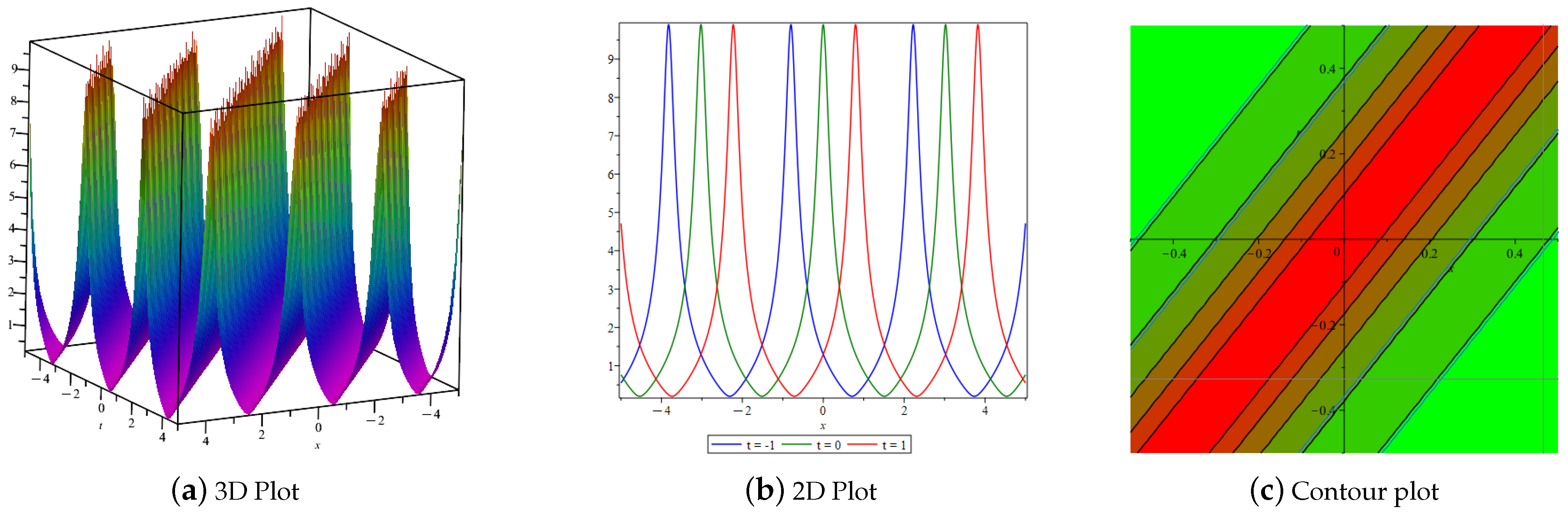
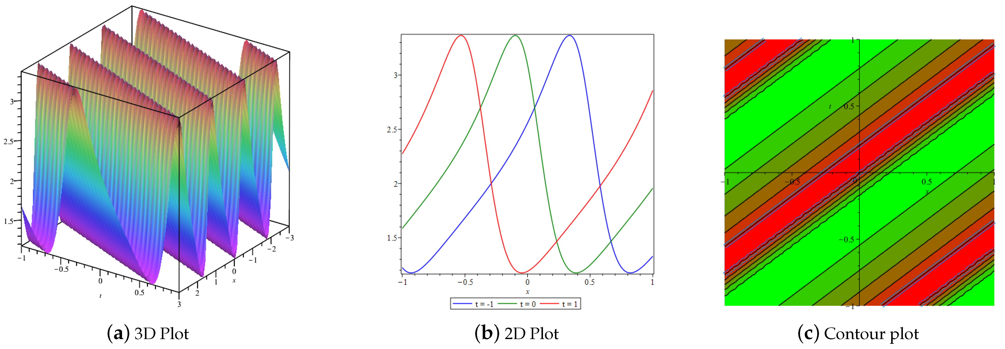
- : When and , thenFigure 5. Graphical visualization of the derived solution of Equation (97) of the NEDAM method, providing periodic wave solutions such as a (a) 3D surface, (b) 2D surface, and (c) contour plot forFigure 5. Graphical visualization of the derived solution of Equation (97) of the NEDAM method, providing periodic wave solutions such as a (a) 3D surface, (b) 2D surface, and (c) contour plot for
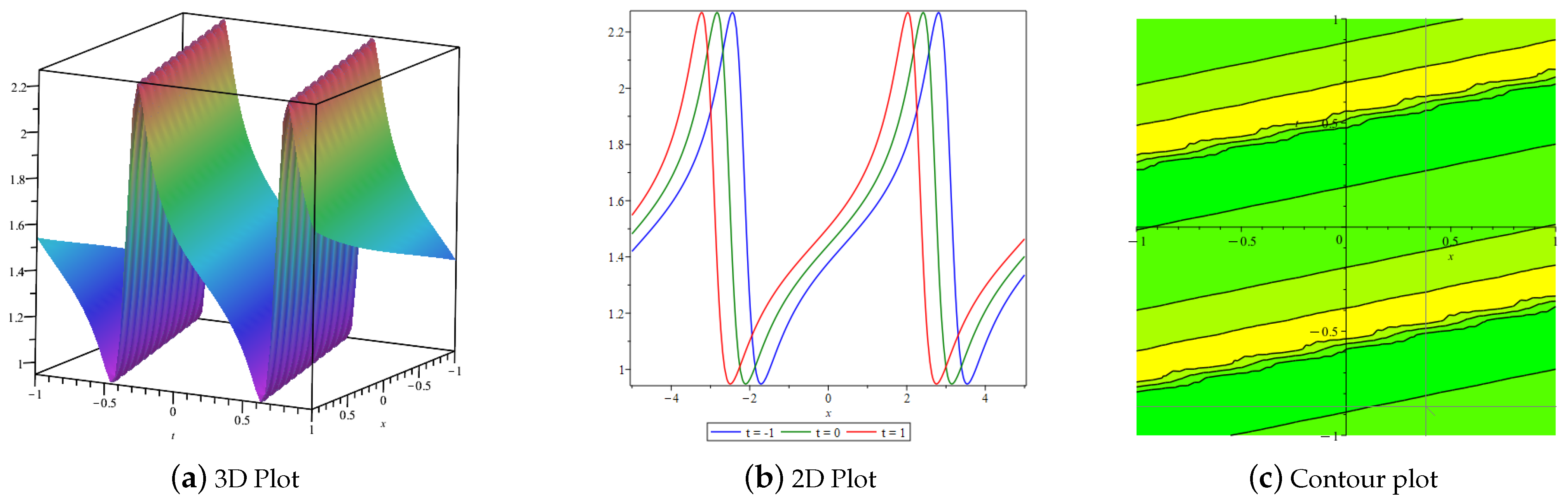
![Axioms 14 00590 g005]() Figure 6. Graphical visualization of the derived solution of Equation (98) of the NEDAM method, providing periodic wave solutions such as a (a) 3D surface, (b) 2D surface, and (c) contour plot forFigure 6. Graphical visualization of the derived solution of Equation (98) of the NEDAM method, providing periodic wave solutions such as a (a) 3D surface, (b) 2D surface, and (c) contour plot for
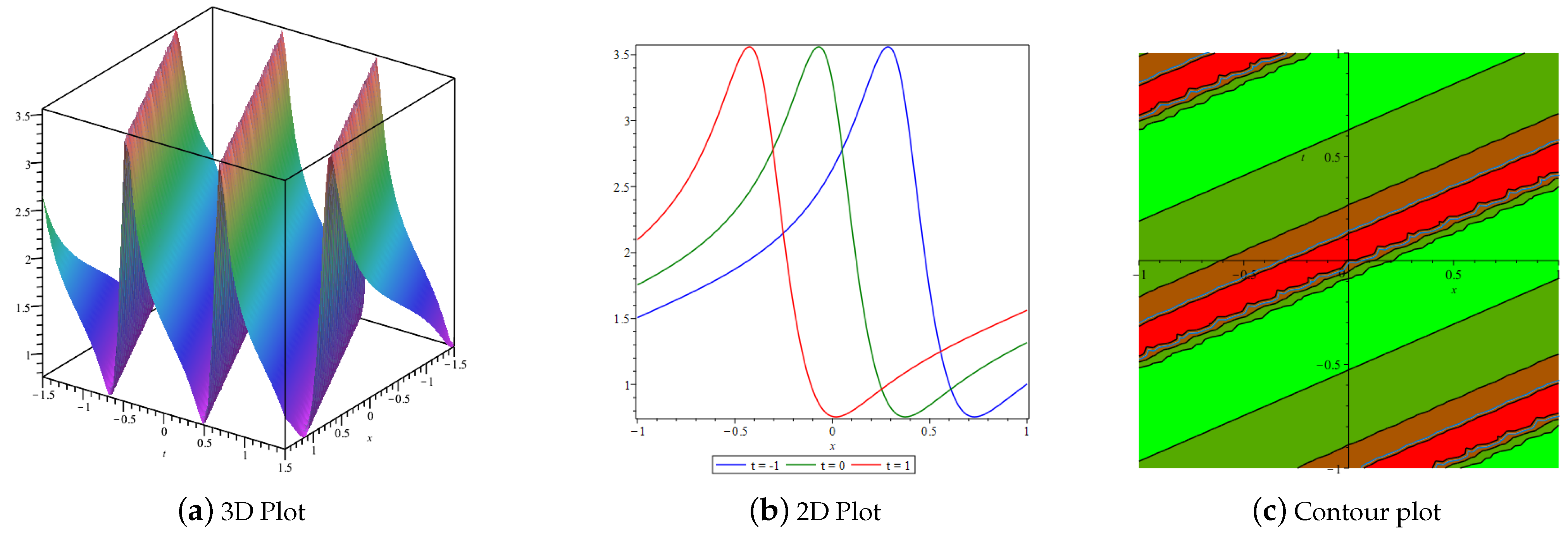
Figure 6. Graphical visualization of the derived solution of Equation (98) of the NEDAM method, providing periodic wave solutions such as a (a) 3D surface, (b) 2D surface, and (c) contour plot forFigure 6. Graphical visualization of the derived solution of Equation (98) of the NEDAM method, providing periodic wave solutions such as a (a) 3D surface, (b) 2D surface, and (c) contour plot for![Axioms 14 00590 g006]() Figure 7. Graphical visualization of the derived solution of Equation (100) of the NEDAM method, providing periodic wave solutions such as a (a) 3D surface, (b) 2D surface, and (c) contour plot forFigure 7. Graphical visualization of the derived solution of Equation (100) of the NEDAM method, providing periodic wave solutions such as a (a) 3D surface, (b) 2D surface, and (c) contour plot for
Figure 7. Graphical visualization of the derived solution of Equation (100) of the NEDAM method, providing periodic wave solutions such as a (a) 3D surface, (b) 2D surface, and (c) contour plot forFigure 7. Graphical visualization of the derived solution of Equation (100) of the NEDAM method, providing periodic wave solutions such as a (a) 3D surface, (b) 2D surface, and (c) contour plot for![Axioms 14 00590 g007]()
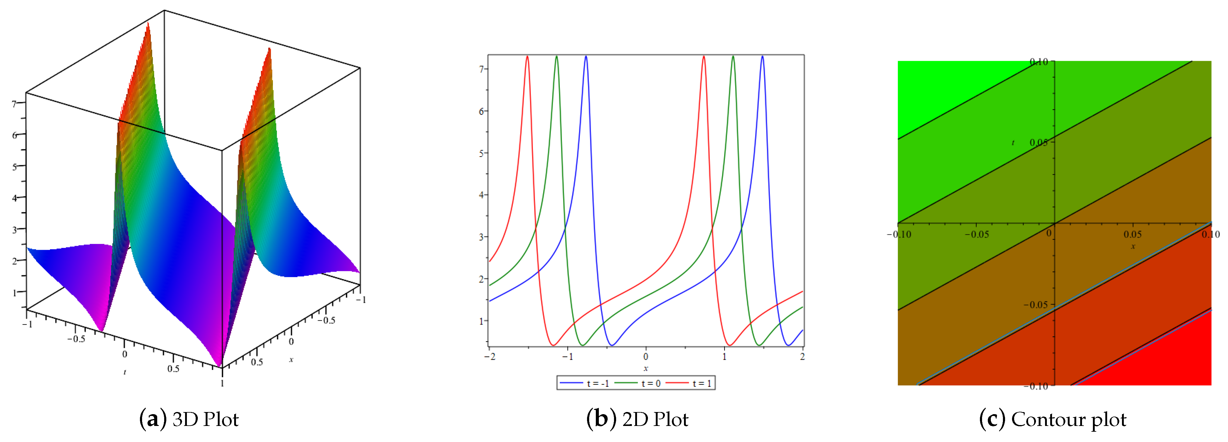
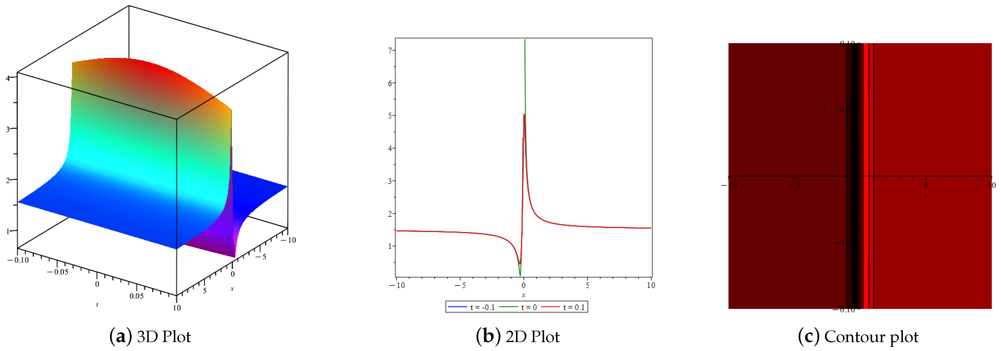
- : When and , thenFigure 8. Graphical visualization of the derived solution of Equation (101) of the NEDAM method, providing periodic wave solutions such as a (a) 3D surface, (b) 2D surface, and (c) contour plot forFigure 8. Graphical visualization of the derived solution of Equation (101) of the NEDAM method, providing periodic wave solutions such as a (a) 3D surface, (b) 2D surface, and (c) contour plot for
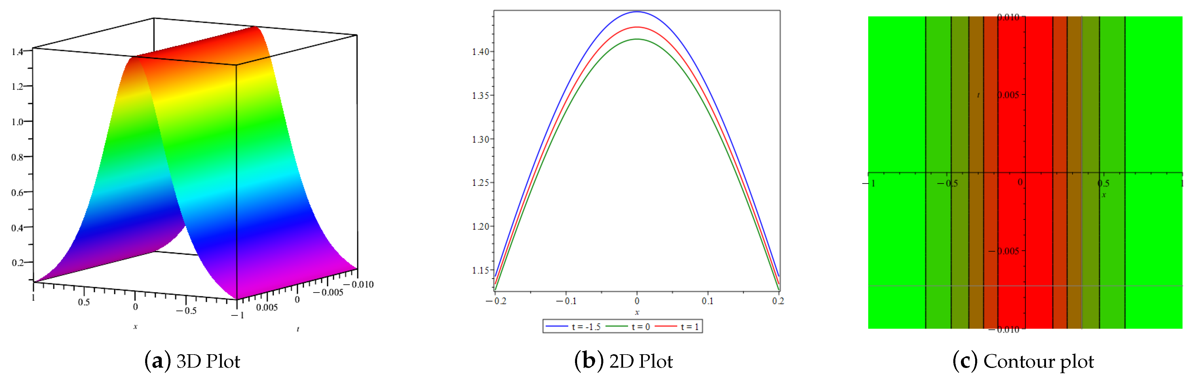
![Axioms 14 00590 g008]() Figure 9. Graphical visualization of the derived solution of Equation (102) of the NEDAM method, providing kink wave solutions such as a (a) 3D surface, (b) 2D surface, and (c) contour plot forFigure 9. Graphical visualization of the derived solution of Equation (102) of the NEDAM method, providing kink wave solutions such as a (a) 3D surface, (b) 2D surface, and (c) contour plot for
Figure 9. Graphical visualization of the derived solution of Equation (102) of the NEDAM method, providing kink wave solutions such as a (a) 3D surface, (b) 2D surface, and (c) contour plot forFigure 9. Graphical visualization of the derived solution of Equation (102) of the NEDAM method, providing kink wave solutions such as a (a) 3D surface, (b) 2D surface, and (c) contour plot for![Axioms 14 00590 g009]()
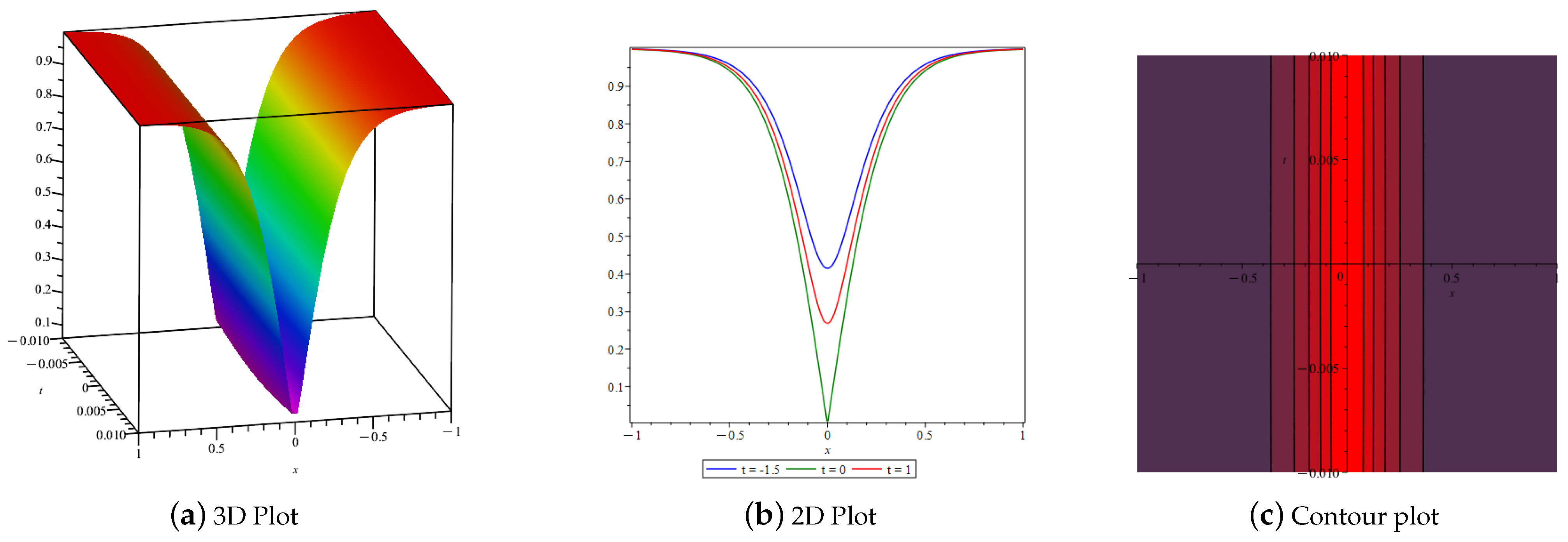
- : When and , thenFigure 10. Graphical visualization of the derived solution of Equation (110) of the NEDAM method, providing dark-bright wave solutions such as a (a) 3D surface, (b) 2D surface, and (c) contour plot forFigure 10. Graphical visualization of the derived solution of Equation (110) of the NEDAM method, providing dark-bright wave solutions such as a (a) 3D surface, (b) 2D surface, and (c) contour plot for
![Axioms 14 00590 g010]()
- : When and , then
- : When and , then
- : When or , then
- : When , and , then
- : When , then
- : When , then
- : When and , then
- : When , , and , then

5. Conclusions
Author Contributions
Funding
Data Availability Statement
Conflicts of Interest
References
- Almatrafi, M.B.; Alharbi, A. New Soliton Wave Solutions to a Nonlinear Equation Arising in Plasma Physics. CMES-Comput. Model. Eng. Sci. 2023, 137, 827–841. [Google Scholar] [CrossRef]
- Hosseini, K.; Hinçal, E.; Ilie, M. Bifurcation analysis, chaotic behaviors, sensitivity analysis, and soliton solutions of a generalized Schrödinger equation. Nonlinear Dyn. 2023, 111, 17455–17462. [Google Scholar] [CrossRef]
- Wangersky, P.J. Lotka-Volterra population models. Annu. Rev. Ecol. Syst. 1978, 9, 189–218. [Google Scholar] [CrossRef]
- Das, S.; Gupta, P.K. A mathematical model on fractional Lotka–Volterra equations. J. Theor. Biol. 2011, 277, 1–6. [Google Scholar] [CrossRef] [PubMed]
- Rezazadeh, H. New solitons solutions of the complex Ginzburg-Landau equation with Kerr law nonlinearity. Optik 2018, 167, 218–227. [Google Scholar] [CrossRef]
- Inc, M.; Iqbal, M.S.; Baber, M.Z.; Qasim, M.; Iqbal, Z.; Tarar, M.A.; Ali, A.H. Exploring the solitary wave solutions of Einstein’s vacuum field equation in the context of ambitious experiments and space missions. Alex. Eng. J. 2023, 82, 186–194. [Google Scholar] [CrossRef]
- Gaillard, P. The mKdV equation and multi-parameters rational solutions. Wave Motion 2021, 100, 102667. [Google Scholar] [CrossRef]
- Ozisik, M. Novel (2+1) and (3+1) forms of the Biswas–Milovic equation and optical soliton solutions via two efficient techniques. Optik 2022, 269, 169798. [Google Scholar] [CrossRef]
- Duran, S. Breaking theory of solitary waves for the Riemann wave equation in fluid dynamics. Int. J. Mod. Phys. B 2021, 35, 2150130. [Google Scholar] [CrossRef]
- Mahmood, I.; Hussain, E.; Mahmood, A.; Anjum, A.; Shah, S.A.A. Optical soliton propagation in the Benjamin–Bona–Mahoney–Peregrine equation using two analytical schemes. Optik 2023, 287, 171099. [Google Scholar] [CrossRef]
- Hosseini, K.; Mirzazadeh, M.; Gómez-Aguilar, J.F. Soliton solutions of the Sasa–Satsuma equation in the monomode optical fibers including the beta-derivatives. Optik 2020, 224, 165425. [Google Scholar] [CrossRef]
- Xiao, Y.; Barak, S.; Hleili, M.; Shah, K. Exploring the dynamical behaviour of optical solitons in integrable kairat-II and kairat-X equations. Phys. Scr. 2024, 99, 095261. [Google Scholar] [CrossRef]
- Chakravarty, S.; Kodama, Y. Soliton solutions of the KP equation and application to shallow water waves. Stud. Appl. Math. 2009, 123, 83–151. [Google Scholar] [CrossRef]
- Hussain, E.; Malik, S.; Yadav, A.; Shah, S.A.A.; Iqbal, M.A.B.; Ragab, A.E.; Mahmoud, H.M.A. Qualitative analysis and soliton solutions of nonlinear extended quantum Zakharov-Kuznetsov equation. Nonlinear Dyn. 2024, 112, 19295–19310. [Google Scholar] [CrossRef]
- Akinyemi, L.; Rezazadeh, H.; Yao, S.W.; Akbar, M.A.; Khater, M.M.A.; Jhangeer, A.; Inc, M.; Ahmad, H. Nonlinear dispersion in parabolic law medium and its optical solitons. Results Phys. 2021, 26, 104411. [Google Scholar] [CrossRef]
- Ren, B.; Ma, W.X.; Yu, J. Characteristics and interactions of solitary and lump waves of a (2+1)-dimensional coupled nonlinear partial differential equation. Nonlinear Dyn. 2019, 96, 717–727. [Google Scholar] [CrossRef]
- Younas, U.; Bilal, M.; Sulaiman, T.A.; Ren, J.; Yusuf, A. On the exact soliton solutions and different wave structures to the double dispersive equation. Opt. Quantum Electron. 2022, 54, 71. [Google Scholar] [CrossRef]
- Sirendaoreji. Unified Riccati equation expansion method and its application to two new classes of Benjamin–Bona–Mahony equations. Nonlinear Dyn. 2017, 89, 333–344. [Google Scholar] [CrossRef]
- Hussain, E.; Arafat, Y.; Malik, S.; Alshammari, F.S. The (2+1)-Dimensional Chiral Nonlinear Schrödinger Equation: Extraction of Soliton Solutions and Sensitivity Analysis. Axioms 2025, 14, 422. [Google Scholar] [CrossRef]
- Cinar, M.; Secer, A.; Ozisik, M.; Bayram, M. Derivation of optical solitons of dimensionless Fokas-Lenells equation with perturbation term using Sardar sub-equation method. Opt. Quantum Electron. 2022, 54, 402. [Google Scholar] [CrossRef]
- Murad, M.A.S. Optical solutions to conformable nonlinear Schrödinger equation with cubic–quintic–septimal in weakly non-local media by new Kudryashov approach. Mod. Phys. Lett. B 2025, 39, 2550063. [Google Scholar] [CrossRef]
- Cai, G.; Wang, Q.; Huang, J. A modified F-expansion method for solving breaking soliton equation. Int. J. Nonlinear Sci. 2006, 2, 122–128. [Google Scholar]
- Farooq, K.; Hussain, E.; Younas, U.; Mukalazi, H.; Khalaf, T.M.; Mutlib, A.; Shah, S.A.A. Exploring the Wave’s Structures to the Nonlinear Coupled System Arising in Surface Geometry. Sci. Rep. 2025, 15, 11624. [Google Scholar] [CrossRef] [PubMed]
- Kabir, M.M.; Khajeh, A.; Abdi Aghdam, E.; Yousefi Koma, A. Modified Kudryashov method for finding exact solitary wave solutions of higher-order nonlinear equations. Math. Methods Appl. Sci. 2011, 34, 213–219. [Google Scholar] [CrossRef]
- Li, Z.; Lyu, J.; Hussain, E. Bifurcation, chaotic behaviors and solitary wave solutions for the fractional Twin-Core couplers with Kerr law non-linearity. Sci. Rep. 2024, 14, 22616. [Google Scholar] [CrossRef]
- Beenish; Hussain, E.; Younas, U.; Tapdigoglu, R.; Garayev, M. Exploring Bifurcation, Quasi-Periodic Patterns, and Wave Dynamics in an Extended Calogero-Bogoyavlenskii-Schiff Model with Sensitivity Analysis. Int. J. Theor. Phys. 2025, 64, 146. [Google Scholar] [CrossRef]
- Shah, S.A.A.; Hussain, E.; Ma, W.X.; Li, Z.; Ragab, A.E.; Khalaf, T.M. Qualitative Analysis and New Variety of Soliton Profiles for the (1+1)-Dimensional Modified Equal Width Equation. Chaos Solitons Fractals 2024, 187, 115353. [Google Scholar] [CrossRef]
- Hosseini, K.; Hincal, E.; Salahshour, S.; Mirzazadeh, M.; Dehingia, K.; Nath, B.J. On the dynamics of soliton waves in a generalized nonlinear Schrödinger equation. Optik 2023, 272, 170215. [Google Scholar] [CrossRef]
- Faridi, W.A.; Iqbal, M.; Mahmoud, H.A. An Invariant Optical Soliton Wave Study on Integrable Model: A Riccati-Bernoulli Sub-Optimal Differential Equation Approach. Int. J. Theor. Phys. 2025, 64, 71. [Google Scholar] [CrossRef]
- Murad, M.A.S.; Mahmood, S.S.; Emadifar, H.; Mohammed, W.W.; Ahmed, K.K. Optical soliton solution for dual-mode time-fractional nonlinear Schrödinger equation by generalized exponential rational function method. Results Eng. 2025, 27, 105591. [Google Scholar] [CrossRef]
- Elboree, M.K. Soliton solutions for some nonlinear partial differential equations in mathematical physics using He’s variational method. Int. J. Nonlinear Sci. Numer. Simul. 2020, 21, 147–158. [Google Scholar] [CrossRef]
- Wazwaz, A.M.; Kaur, L. Optical solitons and Peregrine solitons for nonlinear Schrödinger equation by variational iteration method. Optik 2019, 179, 804–809. [Google Scholar] [CrossRef]
- Kumar, S.; Mohan, B. A generalized nonlinear fifth-order KdV-type equation with multiple soliton solutions: Painlevé analysis and Hirota Bilinear technique. Phys. Scr. 2022, 97, 125214. [Google Scholar] [CrossRef]
- Esen, H.; Ozisik, M.; Secer, A.; Bayram, M. Optical soliton perturbation with Fokas–Lenells equation via enhanced modified extended tanh-expansion approach. Optik 2022, 267, 169615. [Google Scholar] [CrossRef]
- Raza, N.; Salman, F.; Butt, A.R.; Gandarias, M.L. Lie symmetry analysis, soliton solutions and qualitative analysis concerning to the generalized q-deformed Sinh-Gordon equation. Commun. Nonlinear Sci. Numer. Simul. 2023, 116, 106824. [Google Scholar] [CrossRef]
- Ma, W.X. N-soliton solution and the Hirota condition of a (2+1)-dimensional combined equation. Math. Comput. Simul. 2021, 190, 270–279. [Google Scholar] [CrossRef]
- Mustafa, M.A.; Murad, M.A.S. Soliton solutions to the time-fractional Kudryashov equation: Applications of the new direct mapping method. Mod. Phys. Lett. B 2025, 39, 2550147. [Google Scholar] [CrossRef]
- Roshid, M.M.; Rahman, M.; Sheikh, M.; Uddin, M.; Khatun, M.S.; Roshid, H.O. Dynamical analysis of multi-soliton and interaction of solitons solutions of nonlinear model arise in energy particles of physics. Indian J. Phys. 2025, 99, 3409–3421. [Google Scholar] [CrossRef]
- Rehman, H.U.; Iqbal, I.; Subhi A., S.; Mlaiki, N.; Saleem, M.S. Soliton solutions of Klein–Fock–Gordon equation using Sardar subequation method. Mathematics 2022, 10, 3377. [Google Scholar] [CrossRef]
- Kumar, D.; Singh, J.; Kumar, S. Numerical computation of Klein–Gordon equations arising in quantum field theory by using homotopy analysis transform method. Alex. Eng. J. 2014, 53, 469–474. [Google Scholar] [CrossRef]
- Sassaman, R.; Biswas, A. Soliton perturbation theory for phi-four model and nonlinear Klein–Gordon equations. Commun. Nonlinear Sci. Numer. Simulation 2009, 14, 3239–3249. [Google Scholar] [CrossRef]
- Biswas, A.; Zony, C.; Zerrad, E. Soliton perturbation theory for the quadratic nonlinear Klein–Gordon equation. Appl. Math. Comput. 2008, 203, 153–156. [Google Scholar] [CrossRef]
- Biswas, A.; Song, M.; Zerrad, E. Bifurcation analysis and implicit solution of Klein-Gordon equation with dual-power law nonlinearity in relativistic quantum mechanics. Int. J. Nonlinear Sci. Numer. Simul. 2013, 14, 317–322. [Google Scholar] [CrossRef]
- Shahen, N.H.M.; Ali, M.S.; Rahman, M.M. Interaction among lump, periodic, and kink solutions with dynamical analysis to the conformable time-fractional Phi-four equation. Partial. Differ. Equ. Appl. Math. 2021, 4, 100038. [Google Scholar] [CrossRef]
- Hafez, M.G.; Alam, M.N.; Akbar, M. Exact traveling wave solutions to the Klein–Gordon equation using the novel (G’/G)-expansion method. Results Phys. 2014, 4, 177–184. [Google Scholar] [CrossRef]
- Alam, M.d.N.; Bonyah, E.; Fayz-Al-Asad, M.d.; Osman, M.S.; Abualnaja, K.M. Stable and functional solutions of the Klein-Fock-Gordon equation with nonlinear physical phenomena. Phys. Scr. 2021, 96, 055207. [Google Scholar] [CrossRef]
- Seadawy, A.R.; Ali, A.; Zahed, H.; Baleanu, D. The Klein–Fock–Gordon and Tzitzeica dynamical equations with advanced analytical wave solutions. Results Phys. 2020, 19, 103565. [Google Scholar] [CrossRef]
- Ullah, M.S.; Ali, M.Z.; Roshid, H.-O. Bifurcation analysis and new waveforms to the fractional KFG equation. Partial. Differ. Equ. Appl. Math. 2024, 10, 100716. [Google Scholar] [CrossRef]
- Akram, G.; Arshed, S.; Sadaf, M.; Sameen, F. The generalized projective Riccati equations method for solving quadratic-cubic conformable time-fractional Klien-Fock-Gordon equation. Ain Shams Eng. J. 2022, 13, 101658. [Google Scholar] [CrossRef]
- Islam, M.d.E.; Barman, H.K.; Akbar, M.A. Search for interactions of phenomena described by the coupled Higgs field equation through analytical solutions. Opt. Quantum Electron. 2020, 52, 468. [Google Scholar] [CrossRef]
Disclaimer/Publisher’s Note: The statements, opinions and data contained in all publications are solely those of the individual author(s) and contributor(s) and not of MDPI and/or the editor(s). MDPI and/or the editor(s) disclaim responsibility for any injury to people or property resulting from any ideas, methods, instructions or products referred to in the content. |
© 2025 by the authors. Licensee MDPI, Basel, Switzerland. This article is an open access article distributed under the terms and conditions of the Creative Commons Attribution (CC BY) license (https://creativecommons.org/licenses/by/4.0/).
Share and Cite
Uzair, M.; Tedjani, A.H.; Mahmood, I.; Hussain, E. Exact Solutions and Soliton Transmission in Relativistic Wave Phenomena of Klein–Fock–Gordon Equation via Subsequent Sine-Gordon Equation Method. Axioms 2025, 14, 590. https://doi.org/10.3390/axioms14080590
Uzair M, Tedjani AH, Mahmood I, Hussain E. Exact Solutions and Soliton Transmission in Relativistic Wave Phenomena of Klein–Fock–Gordon Equation via Subsequent Sine-Gordon Equation Method. Axioms. 2025; 14(8):590. https://doi.org/10.3390/axioms14080590
Chicago/Turabian StyleUzair, Muhammad, Ali H. Tedjani, Irfan Mahmood, and Ejaz Hussain. 2025. "Exact Solutions and Soliton Transmission in Relativistic Wave Phenomena of Klein–Fock–Gordon Equation via Subsequent Sine-Gordon Equation Method" Axioms 14, no. 8: 590. https://doi.org/10.3390/axioms14080590
APA StyleUzair, M., Tedjani, A. H., Mahmood, I., & Hussain, E. (2025). Exact Solutions and Soliton Transmission in Relativistic Wave Phenomena of Klein–Fock–Gordon Equation via Subsequent Sine-Gordon Equation Method. Axioms, 14(8), 590. https://doi.org/10.3390/axioms14080590