Abstract
This paper presents a stochastic analysis of a two-unit cold standby system incorporating imperfect switching mechanisms. Each unit operates in one of three states: normal, partial failure, or total failure. Employing Markov processes, the study evaluates system reliability by examining the mean time to failure (MTTF) and steady-state availability metrics. Failure and repair times are assumed to follow exponential distributions, while the switching mechanism is modeled as either perfect or imperfect. The results highlight the significant influence of switching reliability on both MTTF and system availability. This analysis is crucial for optimizing the performance of complex systems, such as thermal power plants, where continuous and reliable operation is imperative. The study also aligns with recent research trends emphasizing the integration of preventive maintenance and advanced reliability modeling approaches to enhance overall system resilience.
MSC:
60K10; 90B25; 60H10; 60K05; 68M15
1. Introduction
Standby redundancy is a widely implemented strategy in critical systems to enhance reliability and availability, particularly in high-stakes environments such as thermal and nuclear power plants. Cold standby systems, where one unit remains inactive until required, offer the advantage of reduced wear and tear on backup units. However, the introduction of imperfect switching mechanisms adds complexity, as failures in the switching process may hinder effective transition from a failed unit to the standby unit.
Although previous research has investigated standby system reliability under both controlled and uncontrolled repair conditions, relatively few studies have focused specifically on the impact of imperfect switching mechanisms. This paper aimed to address this gap by analyzing a two-unit, non-identical cold standby system in which switch reliability is treated as a variable parameter. Employing stochastic modeling through Markov processes, we evaluate how imperfect switching influences system availability and mean time to failure (MTTF), providing valuable insights for designing highly reliable systems.
Several earlier studies have explored similar models. For example, Bashir et al. [1] examined a two-unit system with both controlled and uncontrolled repair dynamics. Other works [2,3,4,5,6,7,8,9,10,11,12,13,14,15,16,17,18,19,20,21] have addressed various configurations involving cold standby systems, failures due to human operators or servers, preventive maintenance, and switch reliability issues. Recent studies [18,19,20,21] have further emphasized the importance of integrating preventive maintenance strategies, advanced stochastic modeling, and consideration of imperfect switching to enhance system performance. This study builds upon and extends these investigations by explicitly incorporating switching imperfections into the system model.
Finally, this paper distinguishes between cold, warm, and hot standby configurations, highlighting the unique trade-offs between resource consumption and switching readiness. While hot standby systems enable immediate takeover at the expense of high energy consumption, cold standby systems are more energy-efficient but more vulnerable to the effects of switching failures.
2. System Assumptions
This study examines a two-unit cold standby system consisting of non-identical units, where one unit is operational while the other remains in cold standby. The operational dynamics of the system are based on the following assumptions:
- The system comprises two non-identical units: one active and one in cold standby.
- Each active unit can operate in one of three states: normal, partial failure, or total failure.
- The switching mechanism between units may be either fully functional or defective.
- Upon the failure of the active unit, if the switch functions correctly, the system immediately transfers operation to the standby unit.
- If the switch is defective, the failed active unit cannot be replaced by the standby unit.
- Repairing the switch is prioritized over the replacement or repair of any failed unit.
- Repair times for both the switch and the units follow exponential probability distributions.
- A unit experiencing partial failure will eventually progress to total failure if not repaired.
- A partially failed unit continues to operate, though with degraded performance.
- Once repaired, a unit returns to its normal operational state.
- If a unit undergoing repair for partial failure deteriorates to total failure, the repair process restarts from the beginning.
- If the active unit partially fails while the standby unit is under repair, priority is given to repairing the partially failed unit.
- Repairing partially failed units always takes precedence over totally failed units.
- A unit repaired from total failure resumes operation as either active or standby, depending on the current system status.
2.1. System States and Transitions
The operational behavior of the system is modeled through state transitions that depend on the condition of each unit and the status of the switching mechanism. The key notations used to represent the states are as follows:
- -
- N: Normal operation.
- -
- P: Partial failure.
- -
- F: Total failure.
- -
- S: Standby.
- -
- Sr: Switch under repair.
2.2. Notation
The following symbols are used throughout the analysis:
- -
- αi: Failure rate from normal to partial failure for unit i (i = 1, 2).
- -
- βi: Transition rate from partial to total failure for unit i.
- -
- γi: Repair rate from partial failure to normal for unit i.
- -
- θi: Repair rate from total failure to either normal or standby for unit i.
- -
- µ: Repair rate of the switch.
- -
- p: Probability that the switch successfully connects the standby unit.
- -
- q: Probability of switch failure, with p + q = 1.
The system can transition through multiple states such as the following:
- -
- S0 (N, S): Active unit is normal, backup is standby.
- -
- S1 (P, S): Active unit has a partial failure, backup is standby.
- -
- S2 (F, Sr, S): Active unit fails, switch is being repaired, standby idle.
- -
- S3 (F, N): Standby is activated while the failed unit is under repair.
- -
- S4 (F, P): Standby is partially failed and under repair; failed unit is paused.
- -
- S5 (F, F): Both units are in total failure.
3. Reliability Analysis (MTTF)
In this section, we analyze the system’s mean time to failure (MTTF) under two scenarios: one with an imperfect switching mechanism and the other with a perfect switching mechanism.
3.1. MTTF for System with Imperfect Switch
We used the following transition diagram (Figure 1):
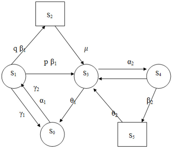
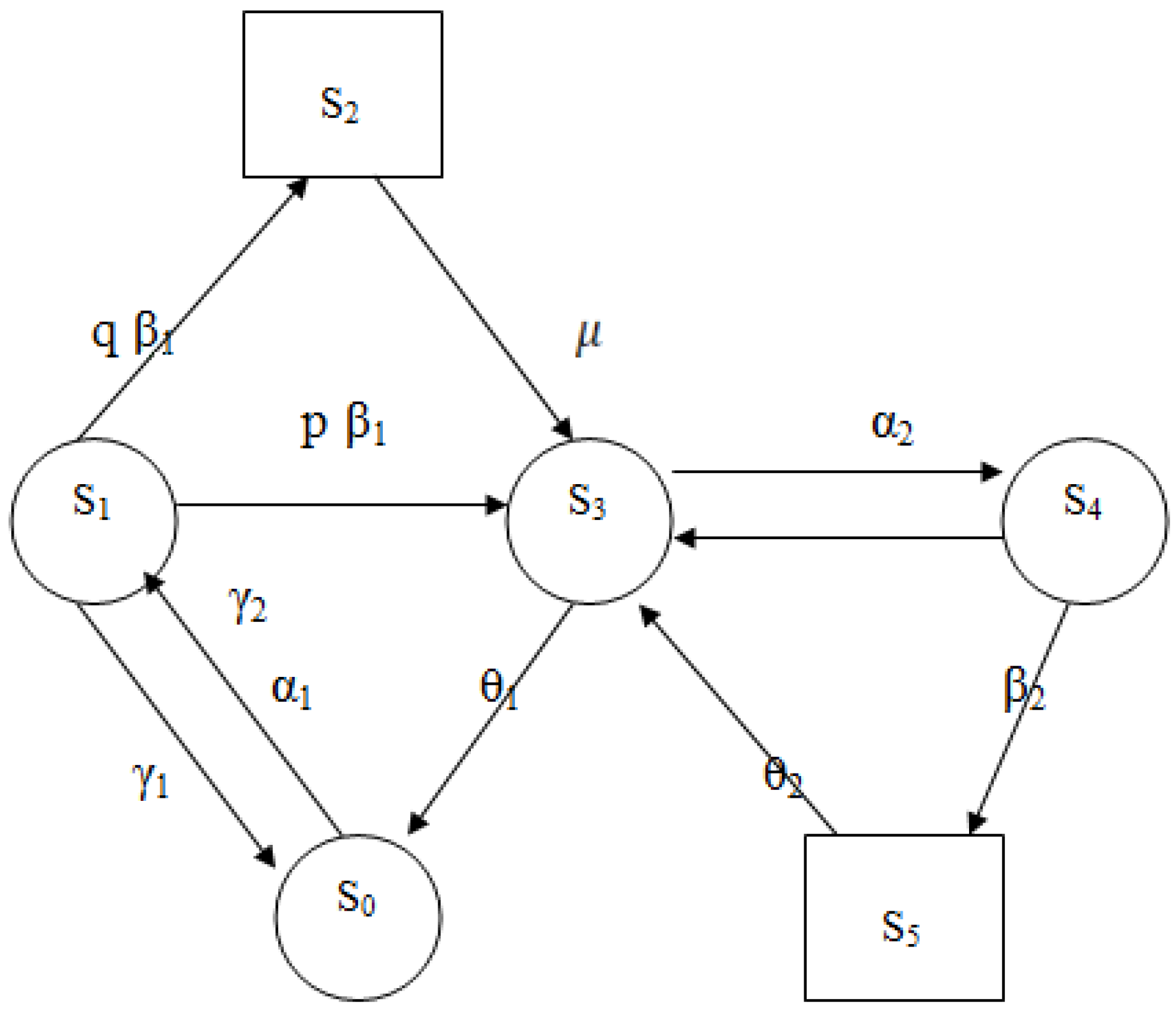
Figure 1.
Transition diagram—imperfect switch.
The system’s behavior is represented through a set of differential equations. The initial probability vector is given as follows:
Assume that the system starts in the fully operational state. States S2 and S5 are considered absorbing. The differential equations can be arranged in matrix form as P’(t) = QP(t), where Q is the generator matrix excluding absorbing states.
Solving for MTTF involves inverting a sub-matrix of Q (denoted as A) and applying the formula
where
where the result gives the expected time to absorption. The derived expression for MTTF in the imperfect switch case is
3.2. MTTF for System with Perfect Switch
In the case of a perfect switch (p = 1), the system transitions are simplified, and only five states are considered.
By substituting p = 1 into the general expression, we obtain a cleaner closed-form formula:
These equations highlight the critical impact of switch reliability. As p increases, the expected system uptime improves significantly.
In the case of a perfect switch (p = 1), the matrix Q is simplified, and the MTTF increases significantly, reflecting enhanced resilience.
4. Availability Analysis
This section analyzes the steady-state availability of the two-unit cold standby system under both imperfect and perfect switching conditions.
4.1. Availability of System with Imperfect Switch
Using the same initial condition vector P(0) = [1, 0, 0, 0, 0, 0], and the system state diagram in Figure 1, we develop a set of differential equations that describe the probability transitions between operational and failed states.
The differential equations form can be expressed as follows:
The steady-state availability A is given by
Or, in the matrix form, it can be stated as follows:
We use the normalizing condition
Then by substituting by (19) in any one of the redundant rows of Q in (18), we have
Solution (20) provides the steady-state availability of the system, the states of which are described by Figure 2, and the explicit expression is
where P4 and P5 represent the probabilities of both units being unavailable. The system of linear equations is solved using the steady-state condition QP(∞) = 0 along with the normalization constraint ∑Pi = 1. The closed-form expression for availability is derived as follows:
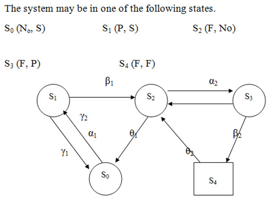
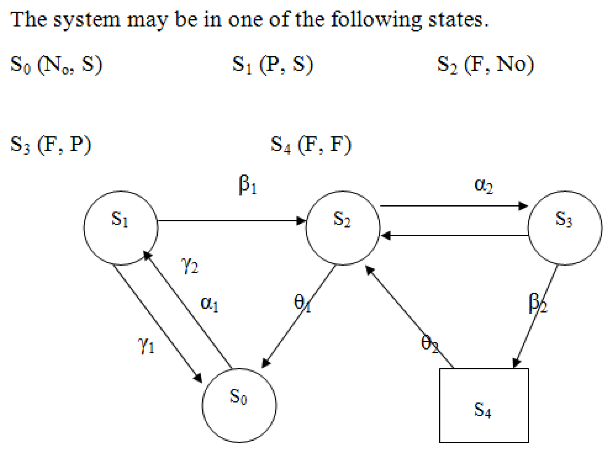
Figure 2.
Transition diagram—perfect switch.
4.2. Availability of System with Perfect Switch
When the switch is perfect (p = 1), we substitute this value into the availability expression, resulting in a simplified form:
where
This refined expression of availability demonstrates unequivocally that enhancing switch reliability leads to higher overall system availability, reaching maximum levels under conditions of perfect switching. This finding holds particular significance for applications where uninterrupted operation is essential, including power generation plants.
Special Case
- -
- The system with two-identical units is as follows:
5. Reliability Modeling and MTTF
5.1. Calculations for System
For Figure 1, we can calculate the MTTF for the system from Equation (9); the explicit expression is given by
5.2. Calculations for System with Perfect Switch
For Figure 2, we can calculate the MTTF for the system from Equation (10); the explicit expression is given by
6. System Availability Investigation
6.1. Computed Values for Imperfect Switch
Derivation of MTTF and Availability Expressions
The derivation of the closed-form expressions for the MTTF and steady-state availability follows a structured Monrovian modeling framework. Initially, the system states were enumerated, incorporating the modes of each unit (normal, partial failure, total failure) and the condition of the switch (functional or defective). For the imperfect switch configuration, the generator matrix Q was formulated by excluding the absorbing states representing total system failure.
A set of coupled differential equations was established to represent the state probabilities over time. These equations are equivalent to the matrix form:
where P (t) is the probability vector
P′ (t) = QP (t)
For the MTTF calculation, the sub-matrix corresponding to transient states was extracted. The expected time to absorption (system failure) was computed using the formula
where P (0) denotes the initial state vector, and 1 is a column vector of ones. This procedure directly led to Equations (9), (10), (22) and (23).
Similarly, the steady-state probabilities were derived by solving
with the normalization condition
QP (∞) = 0,
∑Pi = 1.
This system yielded explicit closed-form formulas for availability, presented as Equations (20), (24) and (25).
Special cases for identical units and perfect switching were obtained by substituting the parameter values (e.g., p = 1) into the general expressions. The full derivation steps are detailed in the original chapter, from constructing the state transition diagram to solving the matrix equations analytically.
For Figure 1, we can calculate the steady-state availability of the system from Equation (20); the explicit expression is given by
where
6.2. Computed Values for Perfect Switch
For Figure 2, we can calculate the steady-state availability of the system from Equation (21); the explicit expression is given by
where
7. System Behavior Through Graphs
To better elucidate the effects of switching reliability and unit configuration, the system’s performance is examined using graphical analyses of the mean time to failure (MTTF) and steady-state availability metrics.
7.1. Non-Identical Units with Imperfect Switch
Figure 3: MTTF vs. failure rate (α1) for p = 0.4, 0.6, 0.8.
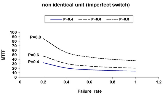
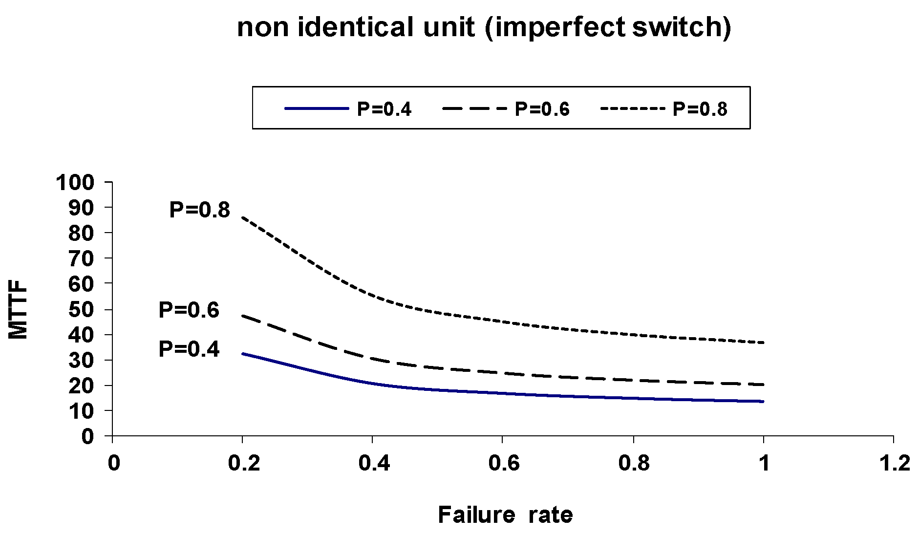
Figure 3.
MTTF versus Failure Rate α1 for Non-Identical Units with Imperfect Switching.
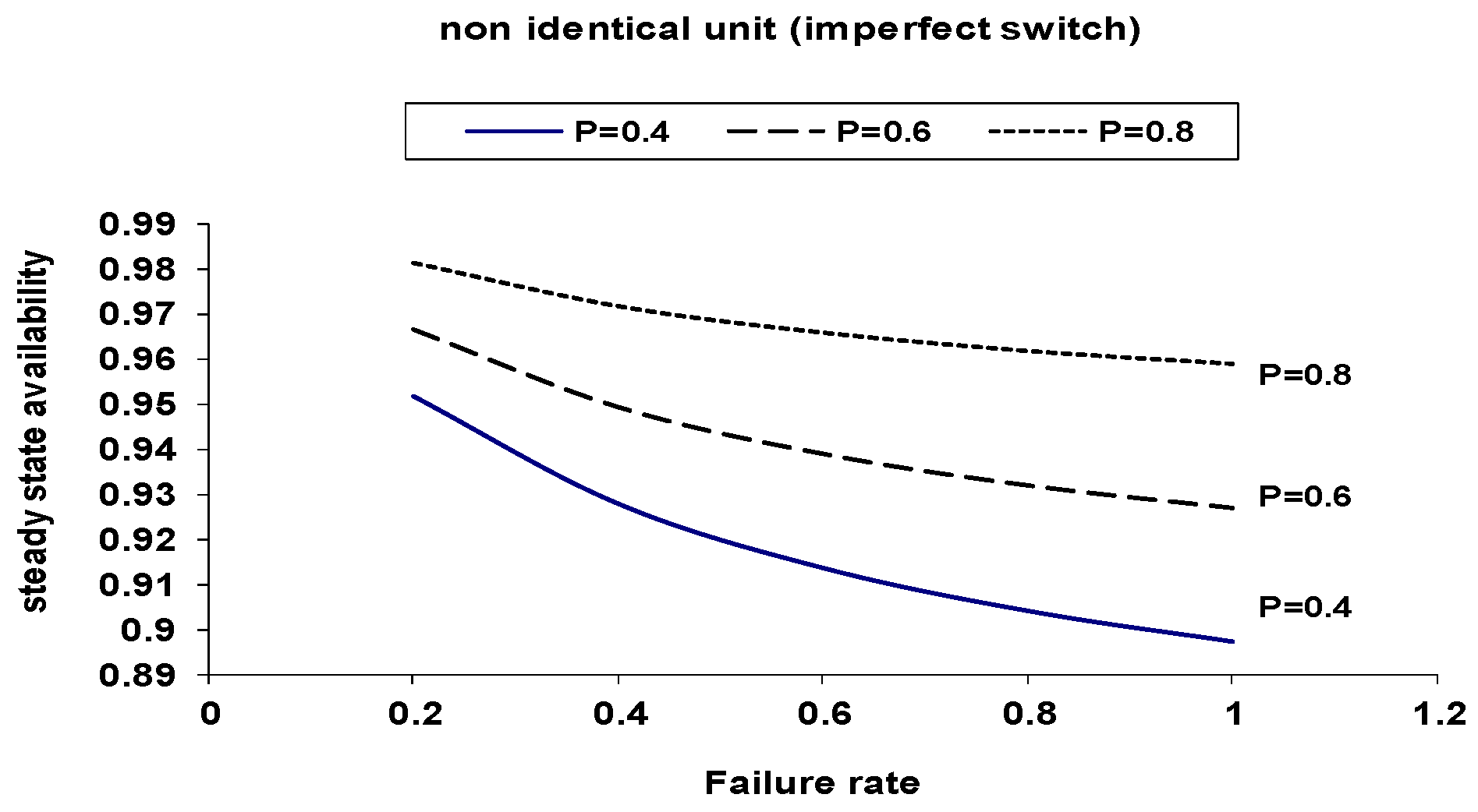
Figure 4: Availability vs. failure rate (α1) for p = 0.4, 0.6, 0.8.
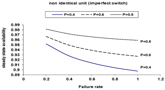
Figure 4.
Steady-State Availability versus Failure Rate α1 for Non-Identical Units with Imperfect Switching.
These graphs show that increasing switch reliability improves both the MTTF and availability, although the system remains sensitive to failure rate changes.
7.2. Identical Units with Imperfect Switch
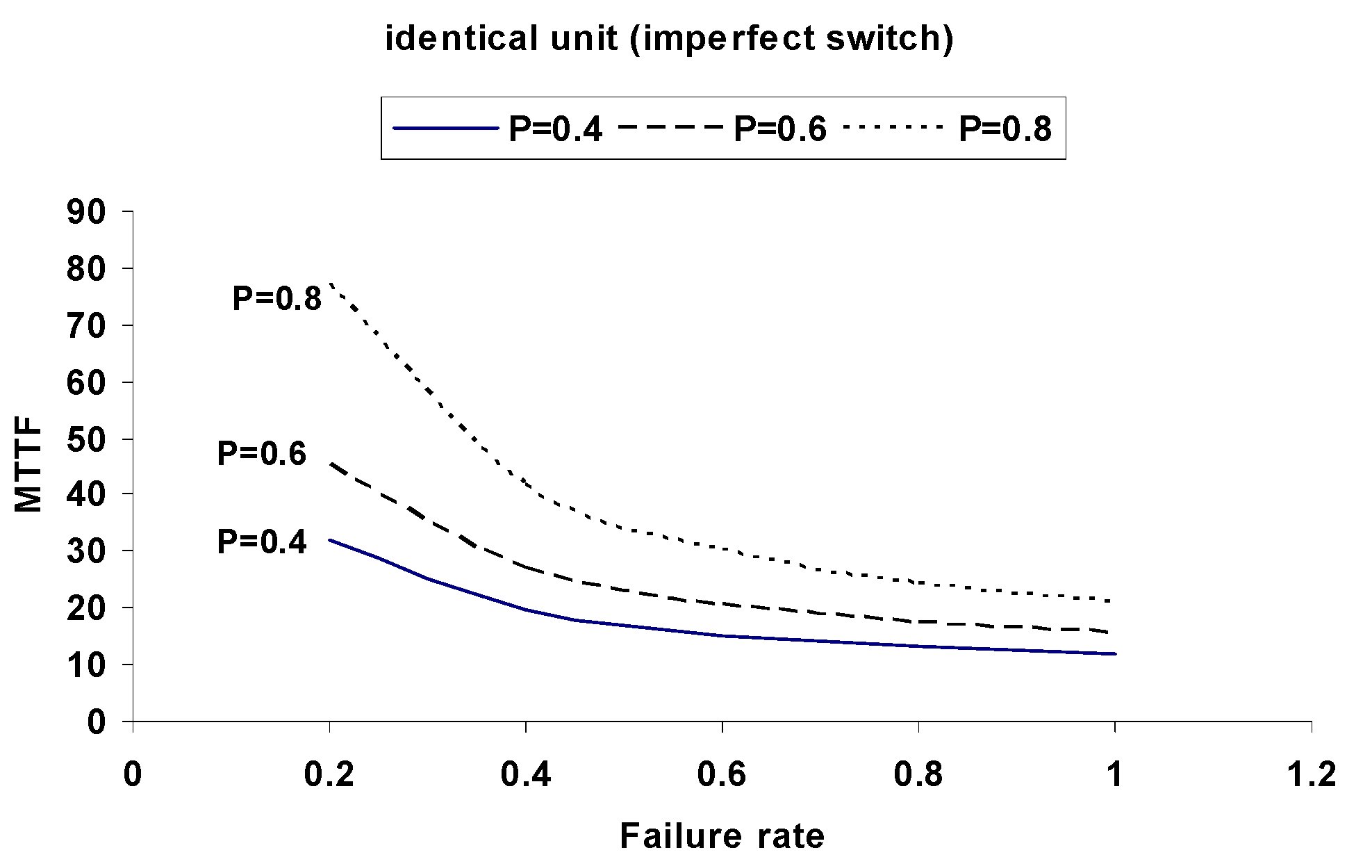
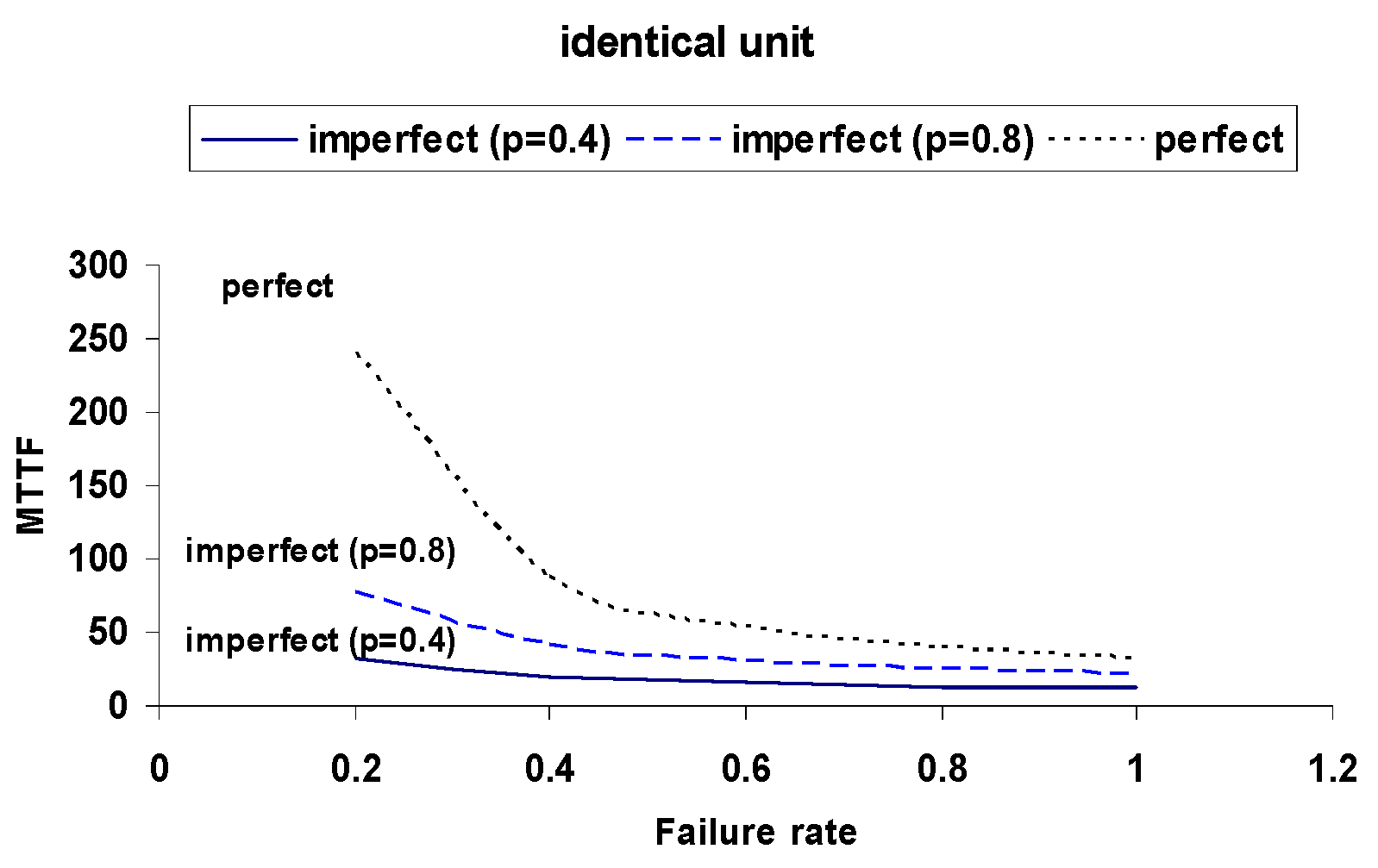
Figure 5: MTTF vs. failure rate (α) for p = 0.4, 0.6, 0.8.
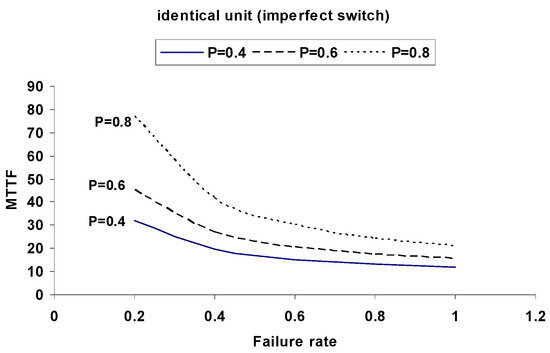
Figure 5.
MTTF versus Failure Rate α for Identical Units with Imperfect Switching.
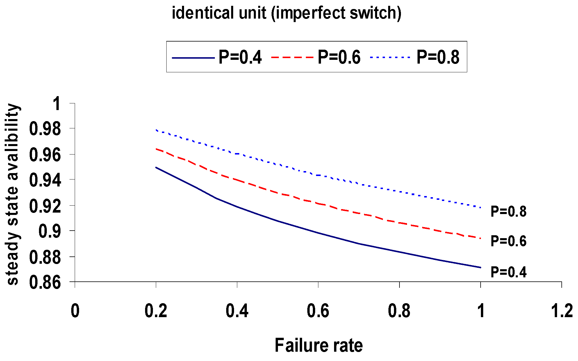
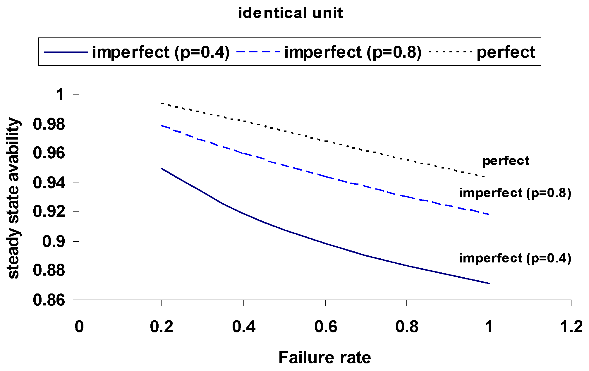
Figure 6: Availability vs. failure rate (α) for p = 0.4, 0.6, 0.8.
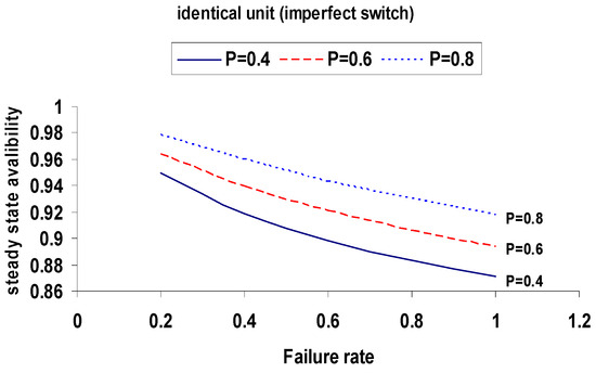
Figure 6.
Steady-State Availability versus Failure Rate α for Identical Units with Imperfect Switching.
Identical units yield higher and more stable MTTF and availability values compared to non-identical units.
7.3. Comparison with Perfect Switch
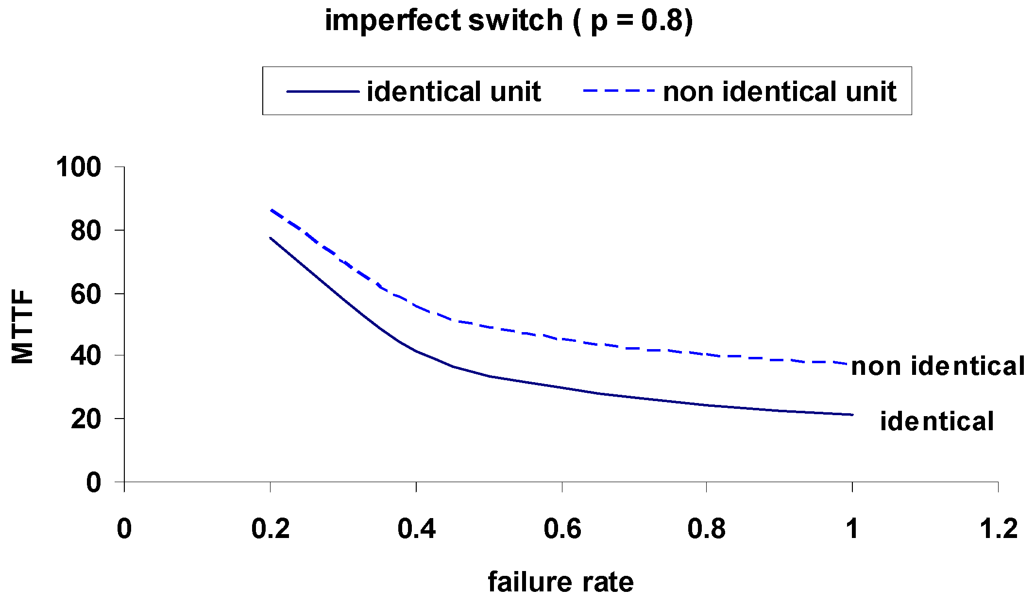
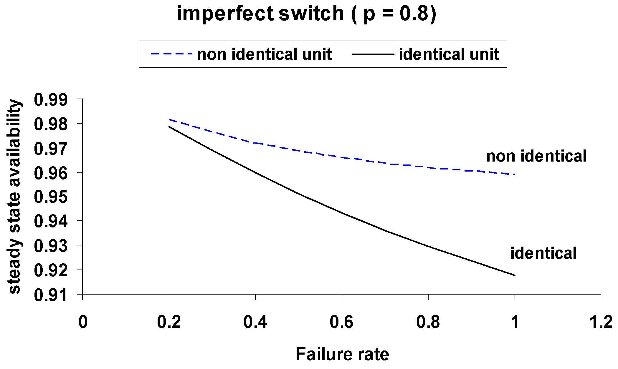
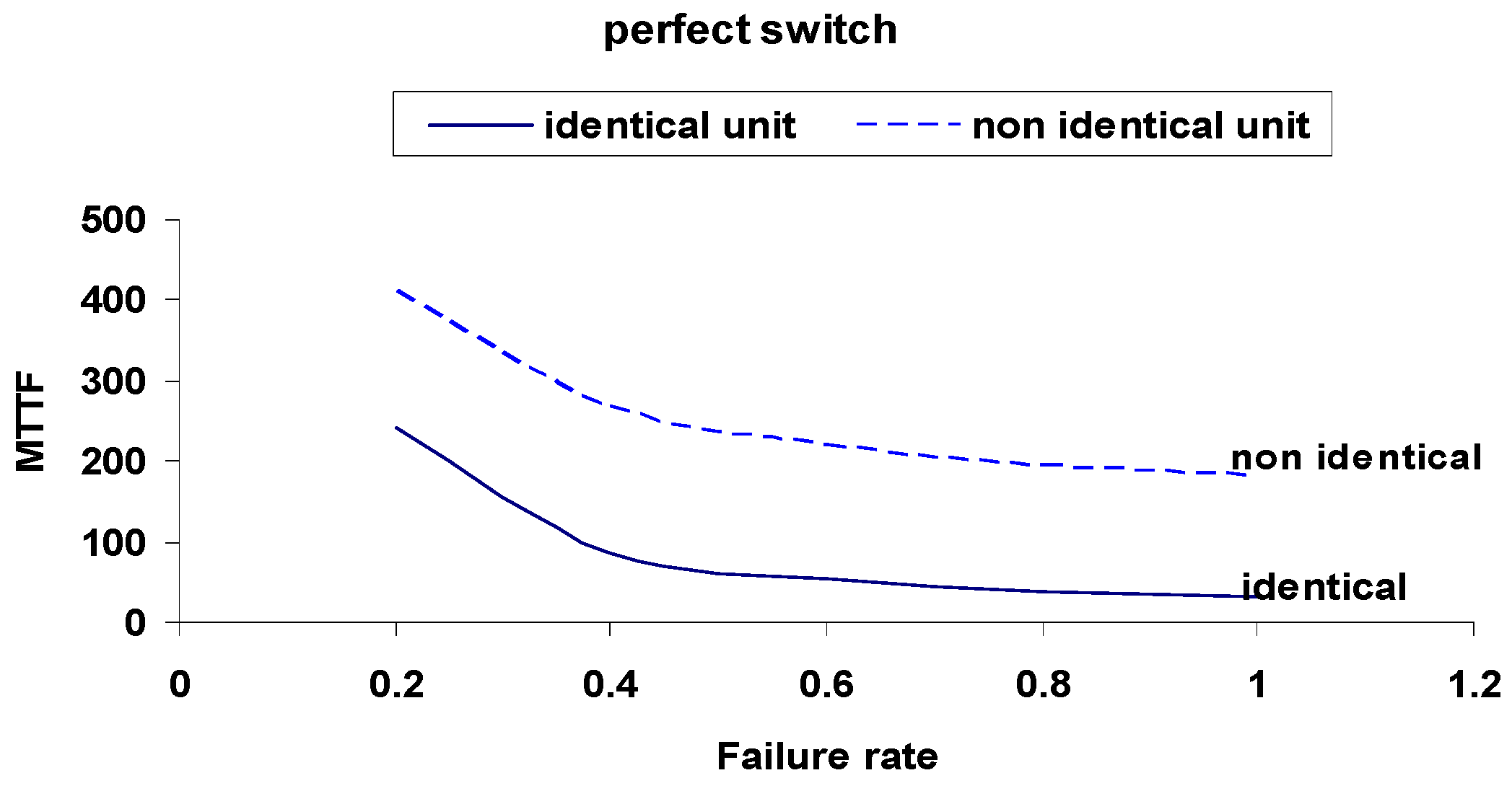
Figure 7 and Figure 8: Comparison of the MTTF and availability between non-identical and identical units at p = 0.8.
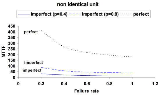
Figure 7.
Comparison of MTTF for Identical and Non-Identical Units with Imperfect and Perfect Switching (p = 0.4, 0.8, 1).

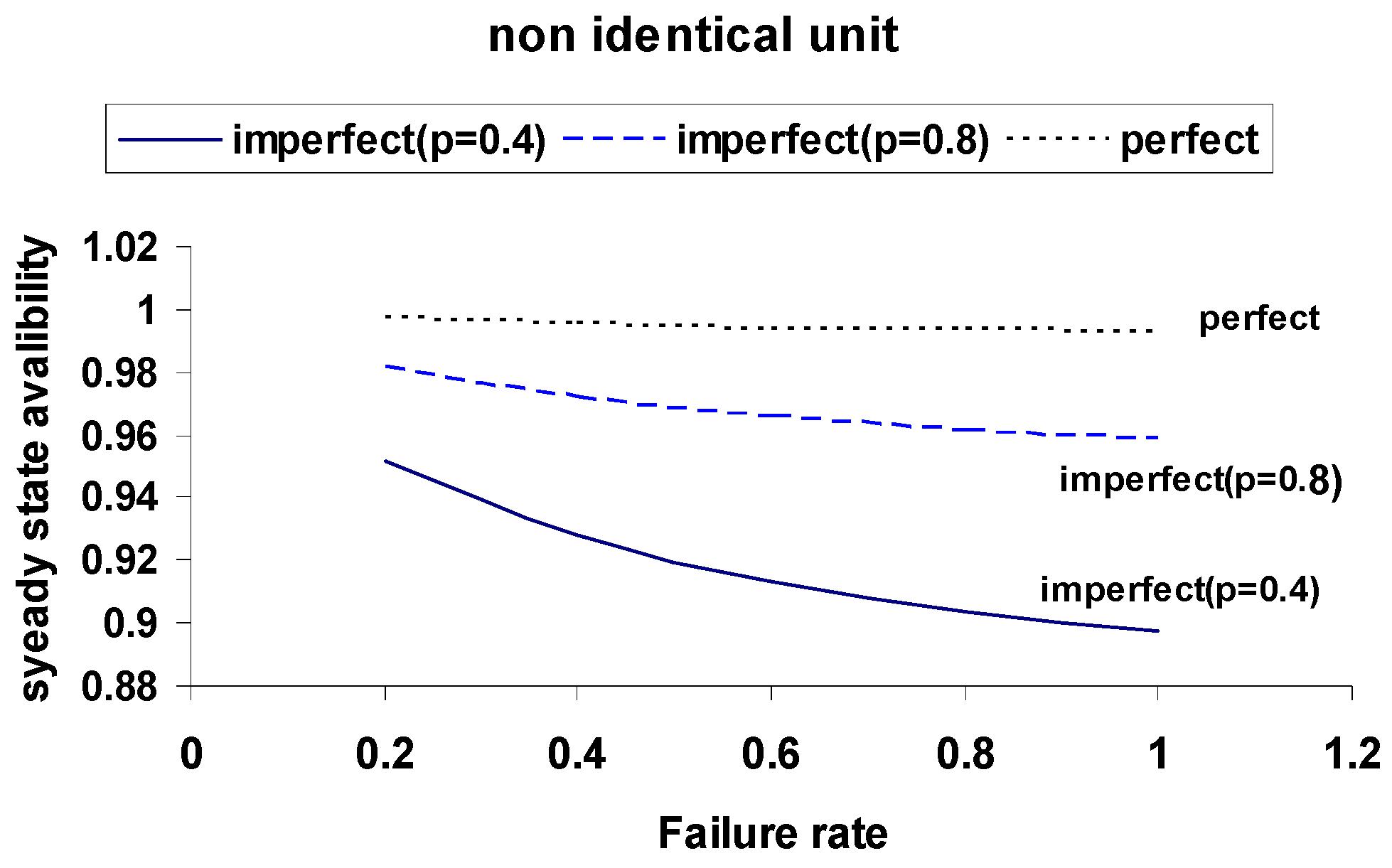
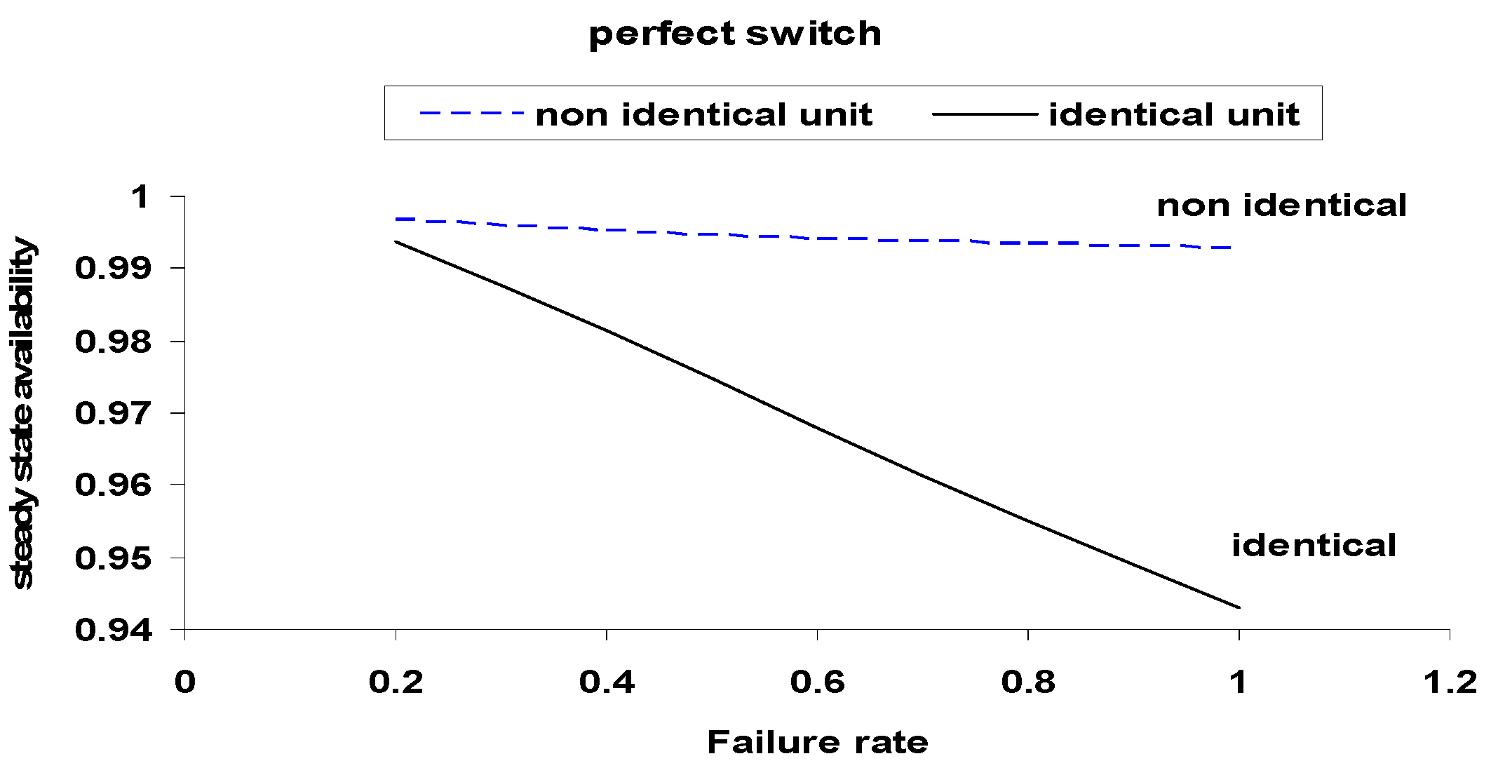
Figure 8.
Comparison of Steady-State Availability for Identical and Non-Identical Units with Imperfect and Perfect Switching.
Figure 9, Figure 10, Figure 11, Figure 12, Figure 13 and Figure 14: MTTF and availability of both unit types under perfect switching (p = 1).
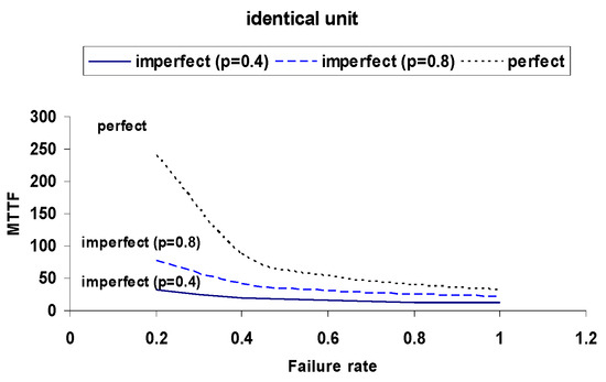
Figure 9.
MTTF versus Failure Rate for Identical Units under Different Switching Probabilities (p = 0.4, 0.8, 1).
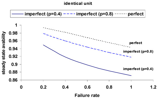
Figure 10.
Steady-State Availability for Identical Units under Different Switching Probabilities.
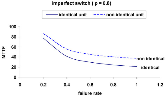
Figure 11.
Comparison of MTTF for Identical and Non-Identical Units with Imperfect Switch (p = 0.8).
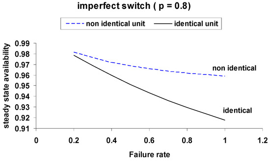
Figure 12.
Comparison of Steady-State Availability for Identical and Non-Identical Units with Imperfect Switch (p = 0.8).
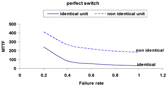
Figure 13.
Comparison of MTTF for Identical and Non-Identical Units with Perfect Switch (p = 1).
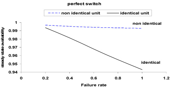
Figure 14.
Comparison of Steady-State Availability for Identical and Non-Identical Units with Perfect Switch.
These comparisons emphasize the substantial improvement in system performance under perfect switching, with identical units achieving the highest metrics. Perfect switches consistently offer better resilience across all failure rates.
Parameter Settings
The following parameters were used to generate the plots:
- -
- For non-identical units: α2 = 0.1, β1 = 0.21, β2 = 0.31, γ1 = 0.41, γ2 = 0.51, θ1 = 0.7, θ2 = 0.8, µ = 0.6.
- -
- For identical units: β1 = β2 = 0.21, γ1 = γ2 = 0.41, θ1 = θ2 = 0.7.
All of the graphs validate the theoretical model, showing the importance of switch reliability and unit similarity in optimizing system performance.
8. Discussion
The analysis clearly demonstrates that the reliability of the switching mechanism has a significant influence on overall system performance. In systems with imperfect switches, both the mean time to failure (MTTF) and steady-state availability degrade noticeably, particularly as the probability of switch failure increases. This degradation is illustrated through the comparison of curves in Figure 3, Figure 4, Figure 5, Figure 6, Figure 7, Figure 8, Figure 9, Figure 10, Figure 11, Figure 12, Figure 13 and Figure 14.
Perfect switching mechanisms lead to consistently higher MTTF and availability values, affirming their importance in critical applications. Non-identical units, due to their variability in failure and repair rates, exhibit more fluctuations and are more sensitive to switching imperfections. Identical units, by contrast, provide more stable performance, especially when coupled with high switch reliability.
These findings are consistent with previous studies, such as Singh et al. [6], which also observed that systems with non-identical units are more prone to performance degradation under imperfect conditions. However, unlike the approach in Bashir et al. [1] and Barak et al. [5], the present work applies Markov modeling techniques to derive closed-form expressions for both the MTTF and steady-state availability. This combination enables a more precise characterization of system behavior across a wider range of failure and switching scenarios.
A notable contribution of this study lies in its systematic comparison of identical and non-identical units under both perfect and imperfect switching configurations, supported by detailed graphical analyses. Prior work, such as Chaudhary and Tomar [4], typically focused on specific configurations (e.g., identical units) or simpler Markov models without explicitly quantifying the incremental improvements offered by perfect switching.
The advantages of this approach include greater modeling flexibility, the ability to capture complex failure dependencies, and enhanced insight into system resilience. For example, compared to the stochastic models proposed by Kadyan et al. [2] and Singh et al. [15], this study provides clearer evidence of how incremental improvements in switch reliability can translate into substantial gains in uptime and reliability metrics. Furthermore, recent research [18,19,20,21] supports the growing need to incorporate factors such as preventive maintenance, repair delays, and imperfect switching into reliability assessments, confirming the relevance of the modeling strategies used in this study.
Overall, the results offer valuable guidance for the design and optimization of critical standby systems, especially in applications where minimizing downtime is essential, such as power generation facilities. Comparisons with the prior literature confirm the relevance of these findings while highlighting the unique contributions and strengths of the proposed methodology.
9. Conclusions
This study underscores the critical role of switching reliability in determining the performance of two-unit cold standby systems. Incorporating imperfect switching mechanisms significantly affects key reliability metrics, including the mean time to failure (MTTF) and steady-state availability. The analytical models demonstrate that even modest improvements in switch reliability can result in substantial gains in system uptime and stability.
Perfect switches, by enabling seamless transitions between units, consistently outperform imperfect counterparts across all tested configurations. Furthermore, systems composed of identical units exhibit superior performance due to their uniform behavior under failure and repair conditions.
These findings are particularly relevant for applications in which uninterrupted service is essential, such as thermal and nuclear power plants. The results highlight the importance of strategic investments in more reliable switching mechanisms or maintenance policies designed to minimize switching failures. These conclusions are aligned with recent studies [18,19,20,21], which emphasize the integration of preventive maintenance and advanced reliability modeling in improving system resilience.
Future research could extend the proposed model to multi-unit systems, incorporate preventive maintenance strategies, or analyze hybrid standby configurations that combine cold and hot redundancy to further enhance reliability and operational efficiency.
Author Contributions
Conceptualization, N.M.R., E.S., A.A.A. and S.S. All authors have read and agreed to the published version of the manuscript.
Funding
This work was supported and funded by the Deanship of Scientific Research at Imam Mohammad Ibn Saud Islamic University (IMSIU) (grant number IMSIU-DDRSP2501).
Data Availability Statement
The original contributions presented in this study are included in the article. Further inquiries can be directed to the corresponding author.
Acknowledgments
This work was supported and funded by the Deanship of Scientific Research at Imam Mohammad Ibn Saud Islamic University (IMSIU) (grant number IMSIU-DDRSP2501).
Conflicts of Interest
The authors declare that there are no conflicts of interest related to the publication of this paper. All research activities were conducted and contributions made in accordance with established ethical standards and principles of academic integrity.
References
- Bashir, N.; Joorel, J.; Jan, T. Reliability Analysis of Two Unit Standby Model with Controlled and Uncontrolled Failure and Replacement Facility. Pak. J. Stat. Oper. Res. 2021, 17, 625–632. [Google Scholar] [CrossRef]
- Kadyan, S.; Malik, S.C.; Gitanjali. Stochastic Analysis of a Three-Unit Non-Identical Repairable System with Simultaneous Working of Cold Standby Units. J. Reliab. Stat. Stud. 2021, 13, 385–400. [Google Scholar] [CrossRef]
- Gahlot, M.; Singh, V.V.; Ayagi, H.I.; Abdullahi, I. Stochastic Analysis of a Two-Units Complex Repairable System with Switch and Human Failure Using Copula Approach. Life Cycle Reliab. Saf. Eng. 2020, 9, 1–11. [Google Scholar] [CrossRef]
- Chaudhary, P.; Tomar, R. A Two Identical Unit Cold Standby System Subject to Two Types of Failures. Reliab. Theory Appl. 2019, 14, 34–43. [Google Scholar]
- Barak, M.S.; Yadav, D.; Kumari, S. Stochastic Analysis of a Two-Unit System with Standby and Server Failure Subject to Inspection. Life Cycle Reliab. Saf. Eng. 2018, 7, 23–32. [Google Scholar] [CrossRef]
- Singh, N.; Singh, D.; Saini, A. Cost-Benefit Analysis of Two Non-Identical Units Cold Standby System Subject to Heavy Rain with Partial Operation After Repair. Glob. J. Pure Appl. Math. 2017, 13, 137–147. [Google Scholar]
- Barak, M.S.; Yadav, D. Stochastic Analysis of a Cold Standby System with Server Failure. Int. J. Math. Stat. Invent. 2016, 4, 18–23. [Google Scholar]
- Ali, U.; Bala, N.; Yusuf, I. Reliability Analysis of a Two Dissimilar Unit Cold Standby System with Three Modes Using Kolmogorov Forward Equation Method. Niger. J. Basic Appl. Sci. 2013, 21, 197–206. [Google Scholar] [CrossRef]
- Manglik, M.; Ram, M. Reliability Analysis of a Two Unit Cold Standby System Using Markov Process. J. Reliab. Stat. Stud. 2013, 6, 65–80. [Google Scholar]
- Ali, U.; Suleiman, K.; Yusuf, I. Mean Time to System Failure and Availability Modeling of a Repairable Non-Identical Three Unit Warm Standby Redundant System. Niger. J. Basic Appl. Sci. 2012, 20, 315–323. [Google Scholar]
- Kumar, A.; Pawar, D.; Malik, S.C. Weathering Server System with Non-identical Units and Priority to Repair of Main Unit. J. Adv. Res. Dyn. Control Syst. 2019, 11, 352–358. [Google Scholar] [CrossRef]
- Bashir, R.; Joorel, J.P.S.; Kour, R. Probabilistic Analysis of Single Unit Model with Controlled and Uncontrolled Demand Factor and Inspection Policy. Int. J. Comput. Theor. Stat. 2016, 3. [Google Scholar]
- Gitanjali; Malik, S.C. Stochastic Behavior of Parallel System with Expert Repair and Maintenance. Soc. Reliab. Saf. 2018, 8, 55–64. [Google Scholar] [CrossRef]
- Kadyan, S.; Barak, M.S.; Gitanjali. Stochastic Analysis of a Non-Identical Repairable System of Three Units with Priority for Operation and Simultaneous Working of Cold Standby Units. Int. J. Stat. Reliab. Eng. 2020, 7, 269–274. [Google Scholar]
- Singh, V.V.; Poonia, P.K.; Adbullahi, A.H. Performance Analysis of a Complex Repairable System with Two Subsystems in Series Configuration with an Imperfect Switch. J. Math. Comput. Sci. 2020, 10, 359–383. [Google Scholar]
- Deswal, S.; Malik, S.C. Reliability Measures of a System of Two Non-Identical Units with Priority Subject to Weather Conditions. J. Reliab. Stat. Stud. 2015, 8, 181–190. [Google Scholar]
- Qiu, Q.; Cui, L.; Shen, J. Availability and Maintenance Modeling for Systems Subject to Dependent Hard and Soft Failures. Appl. Stoch. Models Bus. Ind. 2018, 34, 513–527. [Google Scholar] [CrossRef]
- Sultan, K.S.; Moshref, M.E. Stochastic analysis of a priority standby system under preventive maintenance. Appl. Sci. 2021, 11, 3861. [Google Scholar] [CrossRef]
- Mahmoud, M.A.W.; Rashad, A.M.; Hussien, Z.M. Stochastic analysis of a repairable cold standby system attacked by Poisson shocks considering inspection and post repair. Int. J. Comput. Appl. 2015, 132, 33–40. [Google Scholar] [CrossRef]
- Gupta, R.; Mumtaz, S.Z. Stochastic analysis of a two-unit cold standby system with maximum repair time and correlated failures and repairs. J. Qual. Maint. Eng. 1996, 2, 66–76. [Google Scholar] [CrossRef]
- Zhao, L.; Wang, X. A comprehensive review of reliability modeling for repairable systems with multiple failure modes. Reliab. Eng. Syst. Saf. 2022, 223, 108498. [Google Scholar] [CrossRef]

Disclaimer/Publisher’s Note: The statements, opinions and data contained in all publications are solely those of the individual author(s) and contributor(s) and not of MDPI and/or the editor(s). MDPI and/or the editor(s) disclaim responsibility for any injury to people or property resulting from any ideas, methods, instructions or products referred to in the content. |
© 2025 by the authors. Licensee MDPI, Basel, Switzerland. This article is an open access article distributed under the terms and conditions of the Creative Commons Attribution (CC BY) license (https://creativecommons.org/licenses/by/4.0/).