On the Canonical Form of Singular Distributed Parameter Systems

Abstract

This study addresses the standardization of Singular Distributed Parameter Systems (SDPSs). It focuses on classifying and simplifying first- and second-order linear SDPSs using characteristic matrix theory. First, the study classifies first-order linear SDPSs into three canonical forms based on characteristic curve theory, with an example illustrating the standardization process for parabolic SDPSs. Second, under regular conditions, first-order SDPSs can be decomposed into fast and slow subsystems, where the fast subsystem reduces to an Ordinary Differential Equation (ODE) system, while the slow subsystem retains the spatiotemporal characteristics of the original system. Third, the standardization and classification of second-order SDPSs is proposed using three reversible transformations that achieve structural equivalence. Finally, an illustrative example of a building temperature control is built with SDPSs. The simulation results show the importance of system standardization in real-world applications. This research provides a theoretical foundation for SDPS standardization and offers insights into the practical implementation of distributed temperature systems.

1. Introduction

Various industrial systems, including chemical reaction processes [1], thermal convection [2], acoustic medium model [3], and fluid flows [4], are classified as distributed parameter systems (DPSs). The state of the system changes with both time and space. Therefore, instead of the ODE models given by lumped parameter representation, the state of a DPS is described by partial differential equations (PDEs). SDPSs (also called partial differential algebraic systems (PDAEs) or generalized distributed parameter systems) are a generalization of distributed parameter systems in form. This kind of system has been widely applied in industrial applications [5,6], and the corresponding theoretical research has attracted the attention of many scholars [7,8,9,10,11,12].

Practically, an SDPS is usually used to describe a mixed-type coupled PDE system. The following are two examples of SDSPs.

Example 1.

The following is the Navier–Stokes equation [13]:

$$\begin{array}{ccc}\hfill {\displaystyle \frac{\partial u}{\partial t}}+u·\nabla u+\nabla p-{\displaystyle \frac{1}{R}}{\nabla }^{2}u& =& 0,\hfill \end{array}$$

(1)

$$\begin{array}{ccc}\hfill \nabla ·u& =& 0.\hfill \end{array}$$

(2)

where u is the velocity vector, p is the pressure, ∇ denotes the gradient, and R is the Reynolds number. Equation (1) shows that, as the velocities develop, they are affected not only by a diffusion term ${\nabla }^{2}u$ and an advection term $u·\nabla u$ but also by the pressure gradient $\nabla p$. Equation (2) imposes an algebraic constraint on the system and comes from the continuity equation and the incompressible flow constraint. Let $x={[u,p]}^T$ be the state vector; the system matrix expression form in 1D space is as follows:

$$\left[\begin{array}{cc}1& 0\\ 0& 0\end{array}\right]{\displaystyle \frac{\partial x}{\partial t}}-\gamma \left[\begin{array}{cc}1& 0\\ 0& 0\end{array}\right]{\displaystyle \frac{{\partial }^{2}x}{\partial z^2}}+\left[\begin{array}{cc}u& 1\\ 1& 0\end{array}\right]{\displaystyle \frac{\partial x}{\partial z}}=0.$$

(3)

The linearized form of (3) is

$$\left[\begin{array}{cc}1& 0\\ 0& 0\end{array}\right]{\displaystyle \frac{\partial x}{\partial t}}-\gamma \left[\begin{array}{cc}1& 0\\ 0& 0\end{array}\right]{\displaystyle \frac{{\partial }^{2}x}{\partial z^2}}+\left[\begin{array}{cc}\alpha & 1\\ 1& 0\end{array}\right]{\displaystyle \frac{\partial x}{\partial z}}=0.$$

(4)

The system (4) is a standard linear time-invariant SDPS system.

Example 2.

Chemotaxis system of the parabolic–elliptic type [13].

The so-called Keller–Segel model describes the evolution of chemical populations using parabolic–elliptic systems.

$$\begin{array}{ccc}\hfill u_t& =& \nabla ·\left(D\right(u)\nabla (u\left)\right)-\nabla ·(\chi u\nabla v)+\nabla ·(\xi u\nabla w),x\in \mathrm{\Omega },t>0,\hfill \end{array}$$

(5)

$$\begin{array}{ccc}\hfill 0& =& \Delta v+\alpha u-\beta v,x\in \mathrm{\Omega },t>0,\hfill \end{array}$$

(6)

$$\begin{array}{ccc}\hfill 0& =& \Delta w+\gamma u-\delta w,x\in \mathrm{\Omega },t>0,\hfill \end{array}$$

(7)

$$\begin{array}{ccc}\hfill & & {\displaystyle \frac{\partial u}{\partial n}}={\displaystyle \frac{\partial v}{\partial n}}={\displaystyle \frac{\partial w}{\partial n}},x\in \partial \mathrm{\Omega },t>0.\hfill \end{array}$$

(8)

Here, the unknown functions $u=u(x,t)$,$v=v(x,t)$$w=w(x,t)$ denote the cell density, the concentration of an attractive signal, and the concentration of a repulsive chemical, respectively. Ω is a bounded domain with a smooth boundary $\partial \mathrm{\Omega }$, and ${\displaystyle \frac{\partial }{\partial n}}$ represents the derivative with respect to the outer normal of $\partial \mathrm{\Omega }$. As usual, $\chi ,\xi \ge 0$ and $\alpha ,\beta ,\gamma ,\delta$ are positive parameters, and $D\left(u\right)>0$ is the diffusion coefficient. The system (5)–(8) is a nonlinear SDPS system.

Recent studies have focused on the development of novel mathematical frameworks to describe and analyze SDPSs [13,14,15,16,17,18,19]. One such framework involves the use of backstepping methods and neural operator theory [20] and the adaptive finite element method for distributed elliptic optimal control problems with variable energy regularization [19]. Furthermore, the data-derived method has provided new information on the numerical approximation of SDPSs [20,21,22].

A notable trend in the literature is the exploration of optimal control strategies for SDPSs. Specifically, researchers have investigated linear quadratic optimal control problems in the context of SDPSs, with a focus on handling singularity in the performance index [15]. These studies have led to the development of frequency-based criteria to assess the well-posedness and solvability of optimal control problems [11]. Moreover, the identification of closed-loop optimal solutions under certain conditions has further broadened the scope of optimal control for SDPSs.

Another significant area of research is the application of SDPS to ecological and environmental modeling. The spatial heterogeneity and temporal dynamics inherent in ecological systems make SDPS an ideal framework for studying these complex systems [13]. Researchers have used the flexibility of SDPS models to capture intricate interactions between species, habitats, and environmental factors. This has provided insights into population dynamics, species invasions, and the impact of anthropogenic activities on ecosystems.

In [22], the study extends the DeepONet framework to design backstepping controllers and observers for first-order hyperbolic partial integro-differential equations (PIDEs) with delays and recycling terms. By learning the control kernel functions and observer gains through neural operators, the authors achieve accurate approximations of the control laws, ensuring closed-loop stability. Numerical simulations demonstrate significant computational savings compared to traditional PDE solvers. Ref. [23] analyze finite element discretization for elliptic optimal control problems, introducing a mesh-dependent variable regularization parameter in the energy norm. This approach ensures optimal error estimates in the $L^2\left(\mathrm{\Omega }\right)$ norm, which are particularly beneficial when using adaptive meshes to approximate discontinuous target functions. Numerical results validate the theoretical findings and demonstrate the efficiency of the proposed method. Ref. [21] presents the zeroing dynamics and zeroing-gradient dynamics methods as alternative design approaches for velocity control in hyperbolic distributed parameter systems. Addressing the control singularity problem inherent in traditional methods, the authors demonstrate the effectiveness of their approach through applications to a steam-jacketed heat exchanger and a non-isothermal plug flow reactor. In [24], the study proposes an adaptive spatial model-based predictive control strategy for complex distributed parameter systems (DPSs). By incorporating real-time linearization and adaptive mechanisms, the controller effectively handles the spatial–temporal dynamics of DPSs, enhancing control performance in complex industrial processes. Ref. [25] introduces a reduced-order in-domain control approach for one-dimensional distributed parameter systems modeled within the port-Hamiltonian framework. Ref. [26] addresses the estimation problem in nonlinear systems with actuator and sensor faults by designing a distributed fault-tolerant observer. In [27], the state estimation problem of linear fractional-order singular (FOS) systems is investigated. The researcher demonstrates that the filter and the Riccati equation are stable and converge when an equivalent system is detectable and stabilizable.

SDPSs often refer to different types of PDEs, PDEs and ODEs, and PDEs coupled with algebraic equations. For the same SDPSs, different system parameters or spatial boundary conditions can lead to completely different state results. Therefore, in this study, we assume that all systems are well-posed initial-boundary value problems. Some SDPSs only have generalized solutions, or mild solutions are not considered. Despite this progress, there is still a lack of formal methodologies for the standardization and classification of SDPS in the system-theoretic sense, i.e., methods that provide canonical forms analogous to those in ordinary differential-algebraic systems. This study addresses this gap by developing a characteristic matrix-based framework for simplifying and categorizing first- and second-order linear SDPSs. Specifically, we:

• Classify first-order linear SDPSs into three canonical types based on characteristic curve theory and provide examples such as parabolic-type SDPSs.
• Decompose first-order SDPSs under regularity assumptions into fast (ODE-like) and slow (distributed) subsystems.
• Propose structural equivalence transformations to standardize second-order SDPSs.
• Illustrate the theoretical constructs using a building temperature control system, demonstrating the utility of SDPS standardization in real-world applications.

This research contributes both to the theoretical foundations of SDPS standardization and to the practical implementation of distributed control systems, particularly in fields where spatial–stemporal constraints and algebraic coupling are intrinsic to the system dynamics.

The main content of this study is as follows. First, with the PDE characteristic theory, we analyze the standardization of first-order constant coefficient linear SDPS with two independent variables. Mainly, it uses the theory of the characteristic matrix pair to classify first-order SDPSs into three canonical forms. Specifically, for the parabolic-form SDPSs, we propose an example to intuitively illustrate the standardization process. Second, by extending the simplification of the second-order linear SDPSs of two independent variables, the simplification of the second-order linear SDPSs of two independent variables is studied. Finally, as an illustrative example, we show the necessity of SDPS normalization. The illustrated model is a building temperature SDPS system. With different types of system matrices, the singular distributed temperature control systems show some different dynamical properties.

2. Characteristic and Canonical Forms of First-Order SDPSs

Consider the general form of the first-order linear a space-time SDPS

$$E{\displaystyle \frac{\partial X}{\partial t}}+A{\displaystyle \frac{\partial X}{\partial z}}+BX+C=0$$

(9)

Here $t\in [0,+\infty ),z\in \mathbb{R}$,$X(t,z)\in H^1\left(\mathrm{\Omega }\right)$ are the solution functions vector of the system; $A=\left(a_{ij}(t,z)\right)$ is the spatial derivative matrix of the system, $E=\left(e_{ij}(t,z)\right)$ is the time derivative matrix of the system (singular or non-singular); B is the state variable matrix of the system; and $C=\left(c_{ij}(t,z)\right)$ is the term of the nonhomogeneous matrix.

2.1. System Characteristic Matrix

Inspired by the study of the matrix pair $(sE,A)$ in descriptor systems [8], for SDPSs (9), we first introduce the matrix pair regular theory.

For two given square matrices E and A of the same order, the matrix $(sE-A)$ is referred to as a matrix pencil. Here, $s\in \mathbb{C}$ is a constant. If E and A are square matrices and there exists a constant $s_0$ such that

$$det(s_{0}E-A)\ne 0$$

then the matrix pencil $(sE-A)$ is said to be regular. Clearly, when the matrix pencil $(sE-A)$ is regular, all points except for a finite number in the complex plane satisfy the equation. At this point, the equation

$$det(sE-A)=0$$

is called the characteristic equation of the regular matrix pencil $(sE-A)$. the roots of the characteristic equation are referred to as the generalized eigenvalues of the regular matrix pencil $(sE-A)$; the set of generalized eigenvalues of the regular matrix pencil $(sE-A)$ is generally denoted by $\lambda (E,A)$; and the polynomial $P\left(s\right)=det(sE-A)$ is called the characteristic polynomial of the regular matrix pencil $(sE-A)$. Matrix pencils are divided into two categories: regular and non-regular. Regular matrix pencils have the following properties.

Lemma 1.

The necessary and sufficient condition for the matrix pencil $(sE-A)$ to be regular is that there exist two invertible matrices P and Q such that

$$P\left[EA\right]Q=\left[\begin{array}{ccccc}I& 0& ⋮& A_1& 0\\ 0& E_2& ⋮& 0& I\end{array}\right]$$

where $A_1\in {\mathbb{R}}^{n_1\times n_1}$, $E_2\in {\mathbb{R}}^{n_2\times n_2}$; $E_2$ is a nilpotent matrix.

Definition 1.

For the SDPS system (9), if there exists a curve $\varphi (t,z)=0$ such that the solution of (9) is continuous on the curve, but the first kind of discontinuity exists, in other words, if the curve $\varphi (t,z)=0$ can be used as a weak discontinuous curve of $X(t,z)$, then the first partial derivative of $X(t,z)$ on $\varphi (t,z)=0$ can not be uniquely determined under the constraint $\varphi (t,z)=0$.

Now, we determine the characteristic curve. For a given smooth curve l

$$\left\{\begin{array}{cc}\hfill t=& t\left(\sigma \right),\hfill \\ \hfill z=& z\left(\sigma \right).\hfill \end{array}\right.$$

(10)

$$X(t\left(\sigma \right),z\left(\sigma \right))=F\left(\sigma \right):={(f_1\left(\sigma \right),\cdots ,f_n\left(\sigma \right))}^T$$

where $t\left(\sigma \right),z\left(\sigma \right),F\left(\sigma \right)$ are differentiable functions (function vector) corresponding to the parameter $\sigma$. Considering the weak discontinuous curve

$${\displaystyle \frac{\partial X}{\partial t}}{t}^{\prime }\left(\sigma \right)+{\displaystyle \frac{\partial X}{\partial z}}{z}^{\prime }\left(\sigma \right)=F^{\prime }\left(\sigma \right).$$

(11)

Suppose ${\left(t^{\prime }\left(\sigma \right)\right)}^2+{\left(z^{\prime }\left(\sigma \right)\right)}^2\ne 0$, and substitute (11) in Equation (9); the linear system of ${\displaystyle \frac{\partial X}{\partial z}}$ can be obtained. The determination of this linear system is

$$\mathrm{Det}(A{t}^{\prime }\left(\sigma \right)-E{z}^{\prime }\left(\sigma \right))$$

(12)

Thus, if $\mathrm{Det}(A{t}^{\prime }\left(\sigma \right)-E{z}^{\prime }\left(\sigma \right))\ne 0$ along the curve l, then the partial derivative ${\displaystyle \frac{\partial X}{\partial t}}$, ${\displaystyle \frac{\partial X}{\partial t}}$ can be uniquely determined. Conversely, $Det(A{t}^{\prime }\left(\sigma \right)-E{z}^{\prime }\left(\sigma \right))=0$ or

$$\mathrm{Det}(A-E{\displaystyle \frac{dz}{dt}})=0$$

(13)

imply that ${\displaystyle \frac{\partial X}{\partial t}}$, ${\displaystyle \frac{\partial X}{\partial t}}$ cannot be uniquely determined along the curve l.

2.2. Classification and Standardization of Space-Time First-Order SDPSs

For SDPS (9), let

$$\mathrm{Det}(A-\lambda E)=0$$

(14)

be the general characteristic equation of the system. According to the generalized eigenvalue theory in [8], suppose that (E,A) is regular and impulse-free; then, there exists an invertible matrix $P,Q$ such that

$$PEQ=\left(\begin{array}{cc}{I}_r& 0\\ 0& 0\end{array}\right),PAQ=\left(\begin{array}{cc}{A}_1& 0\\ 0& I_{n-r}\end{array}\right).$$

(15)

This decomposition is called the fast and slow subsystem decomposition. When the system is decomposed into fast and slow subsystems, the slow subsystem usually maintains the original space-time characteristics, while the fast subsystem degenerates into an ordinary differential system. According to the slow subsystem, SDPS (9) is classified as follows.

Definition 2.

An SDPS is strict hyperbolic at each point in the region if and only if the characteristic equation of the slow subsystem $Det(\lambda I_r-A_1)=0$ has different real eigenvalues in this region. If the real roots are not necessarily different from each other, but the eigenvectors corresponding to the eigenvalues are independent of each other, then the SDPS is hyperbolic. If the characteristic equation has no real characteristic root at each point in the region, then it is of the elliptic type.

Example 3.

Consider the following regular SDPS system:

$$\left(\begin{array}{cccc}1& 0& 0& 0\\ 0& 0& 1& 0\\ 0& 0& 0& 0\\ 0& 0& 0& 0\end{array}\right){\displaystyle \frac{\partial X(t,z)}{\partial t}}=\left(\begin{array}{cccc}0& 1& 0& 0\\ 1& 0& 0& 0\\ -1& 0& 0& 0\\ 0& 0& 0& 0\end{array}\right){\displaystyle \frac{\partial X(t,z)}{\partial z}}+\left(\begin{array}{cccc}0& 0& 0& 0\\ 0& 0& 0& 0\\ 0& 0& 0& 1\\ 0& 0& 0& 1\end{array}\right)X(t,z)$$

For the above SDPS, there exist two invertible matrices

$$P=\left(\begin{array}{cccc}1& 0& 1& -1\\ 0& 1& 0& 0\\ 0& 0& -1& 1\\ 0& 0& 1& 0\end{array}\right),Q=\left(\begin{array}{cccc}1& 0& 0& 0\\ -1& -1& 1& 0\\ 0& 1& 0& 0\\ 1& 0& 0& 1\end{array}\right)$$

such that the original SDPS can be transformed into the following slow–fast system

$${\displaystyle \frac{\partial X_1(t,z)}{\partial t}}=\left(\begin{array}{cc}-1& 1\\ 1& 0\end{array}\right){\displaystyle \frac{\partial X_1(t,z)}{\partial z}},0={\displaystyle \frac{\partial X_2(t,z)}{\partial t}}+\left(\begin{array}{cccc}0& 0& 0& 0\\ 1& 0& 0& 1\end{array}\right)X(t,z)$$

(16)

Furthermore, by Def. 2, the original SDPS is of the hyperbolic type because the slow subsystem has the system matrix $\left(\begin{array}{cc}-1& 1\\ 1& 0\end{array}\right)$ with two differential real eigenvalues.

Notes: The decomposition of slow and fast subsystems helps reveal the multi-time-scale structure of singular systems. This is particularly useful for model reduction, control design, and numerical simulation, where fast transients and slow dynamics need to be treated separately for accuracy and efficiency. In singular systems, this decomposition also assists in identifying algebraic constraints and separating differential components from static relationships.

3. Equivalence Analysis of Second Order SDPS

Consider the general second-order linear SDPS

$$A{\displaystyle \frac{{\partial }^{2}X(t,z)}{\partial t^2}}+2B{\displaystyle \frac{{\partial }^{2}X(t,z)}{\partial t\partial z}}+C{\displaystyle \frac{{\partial }^{2}X(t,z)}{\partial z^2}}+\cdots =0.$$

(17)

with state vector $X\left(t,z\right)={\left(x_1\left(t,z\right),x_2\left(t,z\right)\right)}^{\mathrm{T}}$. Here, $\left(t,z\right)$ are the independent variables; $A,B,C\in {\mathbb{R}}^{2\times 2}$ are the coefficient matrices (maybe singular); and ⋯ represent low-order partial derivative parts of the system. Consider another SDPS is represented by

$$A_1{\displaystyle \frac{{\partial }^2\tilde{X}(\tilde{t},\tilde{z})}{\partial {\tilde{t}}^2}}+2B_1{\displaystyle \frac{{\partial }^2\tilde{X}(\tilde{t},\tilde{z})}{\partial \tilde{t}\partial \tilde{z}}}+C_1{\displaystyle \frac{{\partial }^2\tilde{X}(\tilde{t},\tilde{z})}{\partial {\tilde{z}}^2}}+\cdots =0.$$

(18)

Now, we focus on the equivalence relation between SDPSs (17) and (18).

Consider the following three equivalence relation transformations:

(T1): (System Matrix Equivalent Transformation): There exists an invertible matrix P such that

$$A_1=PA,B_1=PB,C_1=PC.$$

(19)

(T2): (State Vector Equivalent Transformation): There exists an invertible matrix Q such that

$$X\left(t,z\right)=Q\tilde{X}(\tilde{t},\tilde{z}),A_1=AQ,B_1=BQ,C_1=CQ.$$

(20)

(T3): (Independent Variables Equivalent Transformation): There exists an invertible matrix $R=\left(\begin{array}{cc}{r}_{11}& r_{12}\\ r_{21}& r_{22}\end{array}\right)$ such that

$${(\tilde{t},\tilde{z})}^{\mathrm{T}}=R(t,z).$$

(21)

And

$$\left\{\begin{array}{cc}\hfill {\displaystyle \frac{{\partial }^2}{\partial t^2}}=& r_{11}^2{\displaystyle \frac{{\partial }^2}{\partial {\tilde{t}}^2}}+2r_{11}{r}_{21}{\displaystyle \frac{{\partial }^2}{\partial \tilde{t}\partial \tilde{z}}}+r_{21}^2{\displaystyle \frac{{\partial }^2}{\partial {\tilde{z}}^2}},\hfill \\ \hfill {\displaystyle \frac{{\partial }^2}{\partial t\partial z}}=& r_{11}{r}_{12}{\displaystyle \frac{{\partial }^2}{\partial {\tilde{t}}^2}}+(r_{11}{r}_{22}+r_{12}{r}_{21}){\displaystyle \frac{{\partial }^2}{\partial \tilde{t}\partial \tilde{z}}}+r_{21}{r}_{22}{\displaystyle \frac{{\partial }^2}{\partial {\tilde{z}}^2}},\hfill \\ \hfill {\displaystyle \frac{{\partial }^2}{\partial z^2}}=& r_{12}^2{\displaystyle \frac{{\partial }^2}{\partial {\tilde{t}}^2}}+2r_{12}{r}_{22}{\displaystyle \frac{{\partial }^2}{\partial \tilde{t}\partial \tilde{z}}}+r_{22}^2{\displaystyle \frac{{\partial }^2}{\partial {\tilde{z}}^2}}.\hfill \end{array}\right.$$

(22)

$$\left\{\begin{array}{c}{A}_1=r_{11}^{2}A+2r_{11}{r}_{21}B+r_{21}^{2}C,\hfill \\ B_1=r_{11}{r}_{12}A+(r_{11}{r}_{22}+r_{12}{r}_{21})B+r_{21}{r}_{22}C,\hfill \\ C_1=r_{12}^{2}A+2r_{12}{r}_{22}B+r_{22}^{2}C.\hfill \end{array}\right.$$

(23)

Definition 3

(SDPS Equivalent Form). If SDPS (17) can be transformed into (18) through three transformations, (T1), (T2), and (T3); then, SDPS (17) is equivalent to (18).

Definition 4

(SDPS Decouplable). If SDPS (17) is equivalent to the following SDPS; then, SDPS (17) is decoupled

$$A_1{\displaystyle \frac{{\partial }^2\tilde{X}(\tilde{t},\tilde{z})}{\partial {\tilde{t}}^2}}+2B_1{\displaystyle \frac{{\partial }^2\tilde{X}(\tilde{t},\tilde{z})}{\partial \tilde{t}\partial \tilde{z}}}+C_1{\displaystyle \frac{{\partial }^2\tilde{X}(\tilde{t},\tilde{z})}{\partial {\tilde{z}}^2}}+\dots =0.$$

(24)

where $A_1=\left(\begin{array}{cc}{\overline{a}}_{11}& 0\\ {\overline{a}}_{21}& {\overline{a}}_{22}\end{array}\right),B_1=\left(\begin{array}{cc}{\overline{b}}_{11}& 0\\ {\overline{b}}_{21}& {\overline{b}}_{22}\end{array}\right),C_1=\left(\begin{array}{cc}{\overline{c}}_{11}& 0\\ {\overline{c}}_{21}& {\overline{c}}_{22}\end{array}\right).$

Theorem 1.

SDPS (17) is decoupled if and only if there exist two non-zero vectors U,V such that

$$UA=\alpha V,UB=\beta V,UC=\gamma V,$$

(25)

where α, β, γ are constants.

Proof. 

Necessary: Suppose that SDPS (17) is decoupled; i.e., SDPS (17) can be transformed into (24) by three transformations (T1), (T2) and (T3). Construct an auxiliary vector $U=(1,0)$; one can get

$$(1,0)A_1=a_{11}(1,0),(1,0)B_1=b_{11}(1,0),(1,0)C_1=c_{11}(1,0).$$

(26)

If $(A_1,B_1,C_1)$ is obtained by the transformations (T1) and (T2), then there existsa non-singular matrix pair $(P,Q)$ such that

$$A_1=PAQ, B_1=PBQ, C_1=PCQ, \left|P\right|\ne 0, \left|Q\right|\ne 0.$$

(27)

Thus, the two non-zero vectors U,V are obtained by

$$U=(0,1)P,V=(1,0)Q^{-1}.$$

(28)

Otherwise, if $(A_1,B_1,C_1)$ are obtained by the transformation (T3), noticing that (23) is an invertible transformation, then the following inverse transformation exists.

$$\left\{\begin{array}{c}A={\overline{r}}_{11}^2{A}_1+2{\overline{r}}_{11}{\overline{r}}_{21}{B}_1+{\overline{r}}_{21}^2{C}_1,\hfill \\ B={\overline{r}}_{11}{\overline{r}}_{12}{A}_1+\left({\overline{r}}_{11}{\overline{r}}_{22}+{\overline{r}}_{12}{\overline{r}}_{21}\right)B_1+{\overline{r}}_{21}{\overline{r}}_{22}{C}_1,\hfill \\ C={\overline{r}}_{12}^2{A}_1+2{\overline{r}}_{12}{\overline{r}}_{22}{B}_1+{\overline{r}}_{22}^2{C}_1.\hfill \end{array}\right.$$

(29)

here $\overline{R}=\left(\begin{array}{cc}{\overline{r}}_{11}& {\overline{r}}_{12}\\ {\overline{r}}_{21}& {\overline{r}}_{22}\end{array}\right)={\left(\begin{array}{cc}{r}_{11}& r_{12}\\ r_{21}& r_{22}\end{array}\right)}^{-1}$ and

$$A_1=\left(\begin{array}{cc}{\overline{a}}_{11}& 0\\ {\overline{a}}_{21}& {\overline{a}}_{22}\end{array}\right),B_1=\left(\begin{array}{cc}{\overline{b}}_{11}& 0\\ {\overline{b}}_{21}& {\overline{b}}_{22}\end{array}\right),C_1=\left(\begin{array}{cc}{\overline{c}}_{11}& 0\\ {\overline{c}}_{21}& {\overline{c}}_{22}\end{array}\right).$$

(30)

Thus, there exist two non-zero vectors U = (1,0), V = (1,0), which meet the conditions.

Sufficiency: If there exist two non-zero vectors U, V that satisfy (25), then we can choose $\left|P\right|\ne 0$, $\left|Q\right|\ne 0$, such that $U=(1,0)P, V=(1,0)Q^{-1}$. Substituting it into (25), one can get

$$(1,0)PA=\alpha (1,0)Q^{-1},(1,0)PB=\beta (1,0)Q^{-1},(1,0)PC=\gamma (1,0)Q^{-1}.$$

(31)

Let $A_1=PAQ,B_1=PBQ,C_1=PCQ$. It follows that

$$A_1=\left(\begin{array}{cc}{\overline{a}}_{11}& 0\\ {\overline{a}}_{21}& {\overline{a}}_{22}\end{array}\right),B_1=\left(\begin{array}{cc}{\overline{b}}_{11}& 0\\ {\overline{b}}_{21}& {\overline{b}}_{22}\end{array}\right),C_1=\left(\begin{array}{cc}{\overline{c}}_{11}& 0\\ {\overline{c}}_{21}& {\overline{c}}_{22}\end{array}\right).$$

(32)

The proof is complete. □

Example 4

(SDPS Decoupling). Consider the following second-order spatiotemporal linear SDPS:

$$\left(\begin{array}{cc}1& 0\\ 0& 1\end{array}\right){\displaystyle \frac{{\partial }^{2}x}{\partial t^2}}+2\left(\begin{array}{cc}0& 1\\ 1& 0\end{array}\right){\displaystyle \frac{{\partial }^{2}x}{\partial t\partial z}}+\left(\begin{array}{cc}1& 0\\ 0& 1\end{array}\right){\displaystyle \frac{{\partial }^{2}x}{\partial z^2}}=0,$$

(33)

Here, $x={[x_1(t,z),x_2(t,z)]}^{\mathrm{T}}$ is the state vector of the SDPS. With system matrix equivalent transformation (T1):

$$P=\left(\begin{array}{cc}{\displaystyle \frac{\sqrt{2}}{2}}& {\displaystyle \frac{\sqrt{2}}{2}}\\ -{\displaystyle \frac{\sqrt{2}}{2}}& {\displaystyle \frac{\sqrt{2}}{2}}\end{array}\right)$$

(34)

and $x=P^{-1}y$, the system (33) is transformed into

$$\left(\begin{array}{cc}1& 0\\ 0& 1\end{array}\right){\displaystyle \frac{{\partial }^{2}y}{\partial t^2}}+2\left(\begin{array}{cc}0& 1\\ 1& 0\end{array}\right){\displaystyle \frac{{\partial }^{2}y}{\partial t\partial z}}+\left(\begin{array}{cc}1& 0\\ 0& 1\end{array}\right){\displaystyle \frac{{\partial }^{2}y}{\partial z^2}}=0,$$

(35)

where $y={(y_1(t,z),y_2(t,z))}^{\mathrm{T}}$. In fact, the system is the combination of the following parabolic PDEs:

$${\displaystyle \frac{{\partial }^2{y}_1}{\partial t^2}}+2{\displaystyle \frac{{\partial }^2{y}_1}{\partial t\partial z}}+{\displaystyle \frac{{\partial }^2{y}_1}{\partial z^2}}=0,{\displaystyle \frac{{\partial }^2{y}_2}{\partial t^2}}+2{\displaystyle \frac{{\partial }^2{y}_2}{\partial t\partial z}}+{\displaystyle \frac{{\partial }^2{y}_2}{\partial z^2}}=0.$$

(36)

Note: The coupling of the system reflects the degree of mutual influence and correlation between several relative systems. However, for the general form SDPS (17), the lower order partial derivative terms cannot generally be decoupled unless special conditions are met. System decoupling is an important method to eliminate coupling between systems, making each system an independent and uncorrelated subsystem.

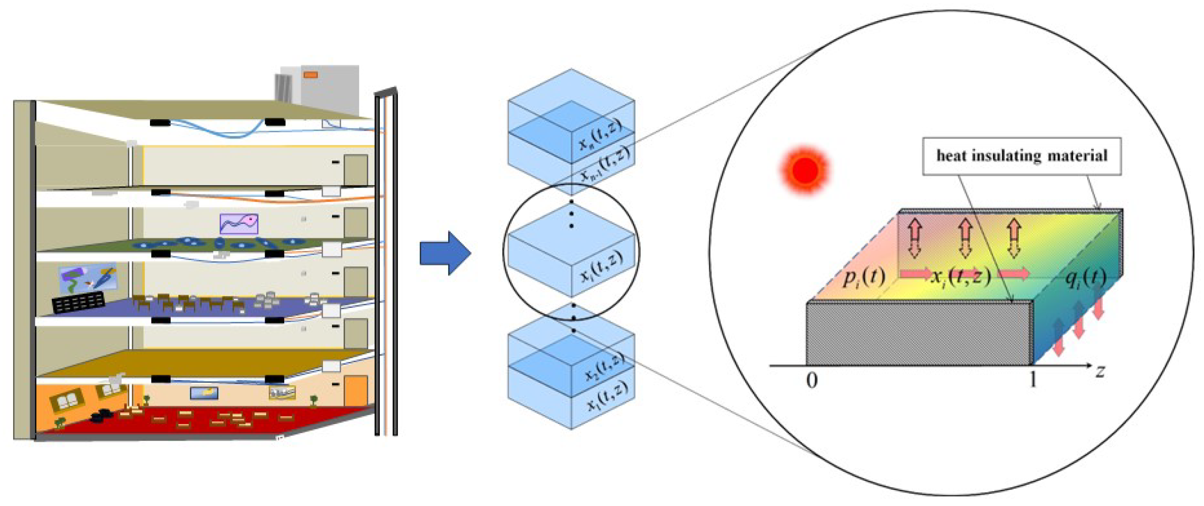
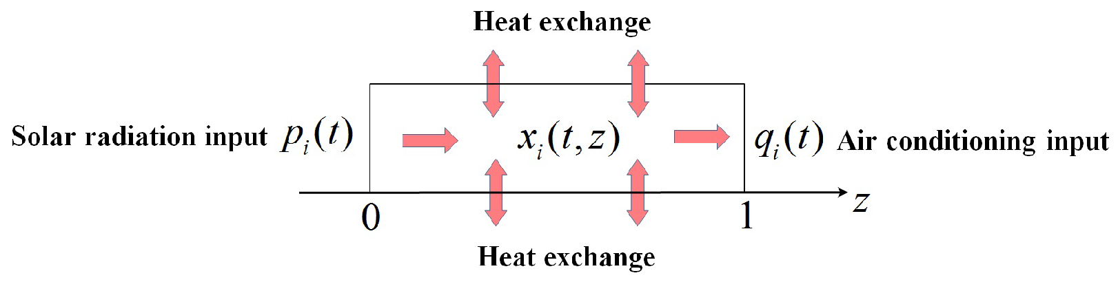
4. Illustrative Example: SDPS Temperature System

Buildings such as company office buildings and university buildings are inhabited by multiple residents who typically have different temperature preferences. Through distributed air conditioning systems, the energy manager can realize collaborative energy and thermal optimization management [28]. In [28], the original model focuses on centralized control strategies, whereas our adaptation incorporates a distributed architecture under the SDPS framework, highlighting its ability to describe the spatio-temporal evolution of the temperature at the floor level. The following SDPS model extends traditional approaches.

In Figure 1, for a building of n stores, let $x_i(t,z)(i=1,\dots ,n)$ represent the spatio-temporal distribution of the temperature of i on the first floor. The discussion focuses on the temperature interaction between multiple modules in addition to the heat balance in a single module. Then, heat transfer on the i-th floor $x_i(t,z)$ can be described by the following parabolic type PDE [15] (See Figure 2).

$${\displaystyle \frac{\partial x_i}{\partial t}}=d_i{\displaystyle \frac{{\partial }^2{x}_i}{\partial z^2}}+a_{i,i}{x}_{i-i}+a_{i,i}{x}_{i,i}+a_{i,i+1}{x}_{i,i+1},t\in R^{+},z\in (0,1)$$

(37)

with boundary conditions in the form of the Dirichlet type,

$$x_i(t,0)=p_i\left(t\right),x_i(t,1)=q_i\left(t\right)$$

(38)

where $d_i$ > 0 is the diffusion coefficient of the i-th floor, which is related to the heat capacity of the medium and the heat transfer rate. Heat exchange between adjacent floors is described by the linear part:

$$a_{i,i-1}{x}_{i-1}(t,z)+a_{i,i}{x}_i(t,z)+a_{i,i+1}{x}_{i+1}(t,z)$$

A special situation is that of special requirements of the floor. For example, the temperature of the j-th floor needs to reach a steady state in a relatively short time.

$${\displaystyle \frac{\partial x_j}{\partial t}}=d_j{\displaystyle \frac{{\partial }^2{x}_j}{\partial z^2}}=a_{j,j-1}{x}_{j-1}+a_{j,j}{x}_j+a_{j,j+1}{x}_{j+1},t\in R^{+},z\in (0,1)$$

(39)

Here, the diffusion coefficient $d_j$ is a large, sufficient, positive number, and $d_j\gg d_i(i\ne j)$. To describe the process accurately, practically, an effective method is to establish the singular perturbation model (with the same method as in [11]). With both sides of Equation (39) divided by $d_j$, one derives

$$\epsilon {\displaystyle \frac{\partial x_j}{\partial t}}={\displaystyle \frac{{\partial }^2{x}_j}{\partial z^2}}+{\displaystyle \frac{a_{j,j-1}}{d_j}}{x}_j+{\displaystyle \frac{a_{j,j}}{d_j}}{x}_j+{\displaystyle \frac{a_{j,j+1}}{d_j}}{x}_{j+1}$$

After the integration of multiple floor temperature subsystems, the following SDPS temperature system is proposed

$$\left\{\begin{array}{l}E{X}_t=D{X}_{zz}+AX,t\in R^{+},z\in (0,1),\\ X(t,0)=P\left(t\right),X(t,1)=Q\left(t\right),t\in R^{+},\\ EX(0,z)=\varphi \left(t\right).\end{array}\right.$$

(40)

Here, $X={[x_1(t,z),\cdots ,x_n(t,z)]}^T$ is the temperature distributed vector of the system. $D=diag(d_1,\cdots ,d_n)$ is the diffusion matrix. The derivative matrix E is a diagonal matrix that possesses the diagonal elements that are identically zero or one. The system’s matrix A has the trigonal type with

$$A=\left[\begin{array}{ccccc}{a}_{11}& a_{12}& & & \\ a_{21}& a_{22}& a_{23}& & \\ & \ddots & \ddots & \ddots & \\ & & a_{n-1,n-2}& a_{n-1,n-1}& a_{n-1,n}\\ & & & a_{n,n-1}& a_{nn}\end{array}\right].$$

The two sides’ input vectors at the left and right boundaries of the system are, respectively,

$$P\left(t\right)={\left(\begin{array}{c}{p}_1\left(t\right),\dots ,p_n\left(t\right)\end{array}\right)}^T,Q\left(t\right)={\left(\begin{array}{c}{q}_1\left(t\right),\dots ,q_n\left(t\right)\end{array}\right)}^T.$$

Practically, these represent the solar radiation input and the air conditioning system input, respectively.

To verify the theoretical results in Section 3, we consider designing the SDPS for a three-layer building temperature distribution system. Specifically, the derivative matrices of the system (40) are set as $E=E_1$ and $E=E_2$ as follows

$$E_1=\left(\begin{array}{ccc}1& 0& 0\\ 0& 1& 0\\ 0& 0& 0\end{array}\right),\mathrm{or}{E}_2=\left(\begin{array}{ccc}1& 0& 0\\ 0& 1& 0\\ 0& 0& 1\end{array}\right).$$

And denote the diffusion matrix D and the system matrix A as

$$D=\left(\begin{array}{ccc}1& 0& 0\\ 0& 2& 0\\ 0& 0& 3\end{array}\right),A=\left(\begin{array}{ccc}2& 2& 0\\ 2& 5& 3\\ 0& 3& 6\end{array}\right).$$

The time-varying boundary temperature inputs are given by

$$P\left(t\right)=\left(\begin{array}{c}1+sin\left(2\pi t\right)\\ 1+sin\left(2\pi t\right)\\ 1+sin\left(2\pi t\right)\end{array}\right)$$

(41)

and

$$Q\left(t\right)=\left(\begin{array}{c}1+cos\left(2\pi t\right)\\ 1+cos\left(2\pi t\right)\\ 1\end{array}\right)$$

(42)

The initial state input $\mathrm{\Phi }\left(z\right)$ is set to

$$\mathrm{\Phi }\left(z\right)=EX(t,z)=\left(\begin{array}{c}1+z(1-z)\\ 1+z(1-z)\\ 0\end{array}\right)$$

(43)

According to the SDPS theory in Section 3, the matrix A has eigenvalues with positive real parts. Therefore, SDPS $(E_1,D,A)$ is parabolic type, while SDPS $(E_2,D,A)$ is parabolic–elliptic type under time-varying boundary inputs $P\left(t\right)$ and $Q\left(t\right)$. We use a second-order accurate finite difference method to discretize the spatial domain $[0,1]$. After spatial discretization, the resulting semi-discrete equations are solved using the ode15s solver in MATLAB (2022) (see

Table 1. Outline of the numerical techniques.

Discretization Schemes	Time Step and Grid Resolution	Relative Error Tolerance
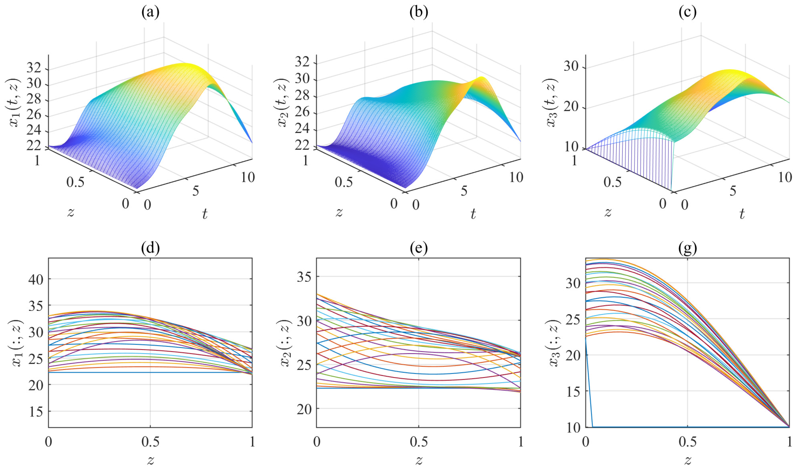
finite difference method	$\Delta t=0.05$, $\Delta x=0.03$	1 × 10−5

for an outline of numerical method parameters).

The simulation results in Figure 3 and Figure 4 intuitively show that the space-time evolution surfaces of the system state variables $x_i(t,z)$ (for $i=1,2,3$) exhibit different properties with different types.

In Figure 3, when the parabolic–elliptic type, the system matrix is $E_1$, the temperature $x_3(t,z)$ instantly reaches a stable state in time and space. However, in Figure 4, with the system matrix of parabolic types $E_2$, the temperature $x_3(t,z)$ evolves slowly.

5. Conclusions

This study mainly studies the standardization problem of SDPS. On the one hand, inspired by the weak discontinuity theory and combined with the restricted equivalence transformation of generalized systems, the concept of characteristic equations for a first-order linear time-invariant SDPS is proposed. Under regular and impulse free constraints, the system can be divided into fast and slow subsystems. The system type depends on the system structure of the slow subsystem. Unlike the general descriptor system, the fast and slow subsystems here are, respectively, the ODE system and the PDE system.

On the other hand, for the second-order SDPS, its standardized equivalent transformation and classification mainly depend on the highest-order partial derivative term coefficient matrix. For the second-order system, there are three reversible structural transformations: system relationship transformation, state variable transformation, and space-time dimension transformation. The equivalent structural transformation of the system depends on the comprehensive results of the three transformations. Finally, in this discussion, the standardization and equivalent transformation theory of the two types of SDPSs cannot be extended directly to the case of time-varying systems. This is primarily due to the significant additional complexities that time-varying parameters introduce, particularly in the analysis of characteristic equations, system stability, and the derivation of canonical forms, which often require fundamentally different mathematical tools and assumptions. Because the system type mainly depends on the highest-order partial derivative term, the conditions for the definite solution of the two types of systems are not discussed here, but under different definite solution conditions, SDPSs have different state responses, and their solution methods are also different.