Article

Equivalence Test and Sample Size Determination Based on Odds Ratio in an AB/BA Crossover Study with Binary Outcomes

1
Department of Statistics and Data Science, Chongqing University of Technology, Chongqing 400054, China
2
Department of Statistics, The Chinese University of Hong Kong, Hong Kong, China
*
Author to whom correspondence should be addressed.
Axioms 2025, 14(8), 582; https://doi.org/10.3390/axioms14080582
Submission received: 30 June 2025 / Revised: 20 July 2025 / Accepted: 25 July 2025 / Published: 27 July 2025
(This article belongs to the Special Issue Recent Developments in Statistical Research)

Abstract

Crossover trials are specifically designed to evaluate treatment effects within individual participants through within-subject comparisons. In a standard AB/BA crossover trial, participants are randomly allocated to one of two treatment sequences: either the AB sequence (where patients receive treatment A first and then cross over to treatment B after a washout period) or the BA sequence (where patients receive B first and then cross over to A after a washout period). Asymptotic and approximate unconditional test procedures, based on two Wald-type statistics, the likelihood ratio statistic, and the score test statistic for the odds ratio (OR), are developed to evaluate the equality of treatment effects in this trial design. Additionally, confidence intervals for OR are constructed, accompanied by an approximate sample size calculation methodology to control the interval width at a pre-specified precision. Empirical analyses demonstrate that asymptotic test procedures exhibit robust performance in moderate to large sample sizes, though they occasionally yield unsatisfactory type I error rates when the sample size is small. In such cases, approximate unconditional test procedures emerge as a rigorous alternative. All proposed confidence intervals achieve satisfactory coverage probabilities, and the approximate sample size estimation method demonstrates high accuracy, as evidenced by empirical coverage probabilities aligning closely with pre-specified confidence levels under estimated sample sizes. To validate practical utility, two real examples are used to illustrate the proposed methodologies.

1. Introduction

In a parallel-group trial design, each participant is randomly assigned to receive a single experimental treatment. This methodology serves as a cornerstone of clinical research, particularly in medical and health science investigations, due to its ability to isolate treatment effects through randomization. By contrast, crossover trials employ a distinct approach wherein each participant sequentially receives multiple experimental treatments under controlled conditions, enabling within-subject comparisons while minimizing inter-individual variability. The design’s methodological strength stems from its ability to isolate treatment effects through paired within-subject comparisons, enhancing both statistical precision and resource efficiency in clinical investigations (Hills and Armitage [1]; Fleiss [2]; Senn [3]). It can significantly reduce both costs and required sample sizes due to within-patient comparison (Sever et al. [4]). For example, in a study by Ménard et al. [5], a crossover design with alternating 2-week active treatment phases and 2-week placebo washout periods was employed to assess antihypertensive efficacy. Their findings indicated that a reduction of 5 mmHg in diastolic blood pressure between active treatment and placebo could be detected with 27 clinic patients and 20 self-monitored home patients under usual statistical risk ( α = 0.05 , β = 0.10 ). At the conclusion of the 3-month follow-up period, each participant could continue receiving the treatment that was the most effective and the best tolerated. This demonstrates that implementing a crossover trial design (with 15-day washout periods between active treatments) combined with precise blood pressure recording not only minimizes the number of patients required for hypertension trials but also enables personalized treatment optimization for individual patients. Recent work by Grenet et al. [6] established that when within-patient correlation ranges from 0.5 to 0.9, crossover trials require only 5–25% as many participants as parallel-group trials to achieve equivalent statistical power for detecting interaction effects.
Crossover trials are commonly utilized in clinical research to compare treatments for chronic diseases. This design is particularly valuable when evaluating new versus existing therapies, as seen in conditions such as asthma and hypertension. The choice of sequences in crossover designs depends on treatment number, sequence length, and trial objectives. The simplest design is the AB/BA crossover, where participants are randomized to either AB or BA sequences to receive two treatments. For the AB treatment group, patients first receive treatment A and then cross over to treatment B after a washout period; for the BA treatment group, patients first receive treatment B and then cross over to treatment A after a washout period. The AB/BA crossover design is also known as a simple crossover or 2 × 2 design (Jones and Kenward [7]). Due to its simplicity, the AB/BA crossover design constitutes a substantial portion of crossover trials in practice (Hills and Armitage [1]; Senn [3,8]; Mills et al. [9]). For example, Fava and Patel [10] reported that over half of 72 crossover trials in a survey of 12 major U.S. pharmaceutical companies used this design (Jones and Kenward [11]).
Significant and productive research has focused on AB/BA crossover trial designs. Under the assumption that carryover effects are absent (typically ensured by an adequate washout period eliminating the impact of the first-stage treatment on the second stage), Kershner and Federer [12] compared the variances for direct, residual, and cumulative treatment effects in two-treatment crossover designs. They considered variance estimates for the second-order residual effects and the interaction effects between period and first-order residuals. To analyze ordinal categorical data from AB/BA crossover trials, Ezzet and Whitehead [13] fitted a random effects model and used the Newton–Raphson algorithm for maximum likelihood estimation. For binomial data, Becker and Balagtas [14] developed likelihood-based methods for hypothesis testing and parameter estimation using two models: a log-linear model for marginal response probabilities and a linear model for log-odds ratios. For AB/BA crossover trials with continuous data, Jaki, Pallmann, and Wolfsegger [15] developed three parameter estimation methods and derived corresponding confidence intervals assuming a normal distribution. Lui and Chang [16] addressed methodological issues in hypothesis testing and parameter estimation for AB/BA crossover trials with ordinal outcomes.
Recently, Lui [17] investigated methods for testing inequality, non-inferiority, and equivalence of treatment effects across continuous, ordinal, binomial, and count data types. The author also provided interval estimation methods for the mean difference between two treatments and explored sample size estimation formulas using the power of the tests. Furthermore, the findings on AB/BA crossover designs were extended to crossover designs involving multiple treatments. Li et al. [18] developed a likelihood ratio test and score test for assessing non-inferiority or equivalence specifically based on the square root of the odds ratio in binomial data in AB/BA crossover trials. Lui [19,20], Lui and Chang [21] developed large-sample and exact small-sample testing procedures for equivalence and non-inferiority assessments of binomial and ordinal categorical data in incomplete block crossover designs. Using Monte Carlo simulations with maximum likelihood estimation, Zhu and Lui [22] quantified the effects of violated normality assumptions for random effects on hypothesis testing and parameter estimation in logistic regression models analyzing binomial data in AB/BA crossover designs. Although extensive research exists on treatment effects in AB/BA crossover trials, there remains a need to investigate equivalence testing based on odds ratios (OR), develop corresponding confidence intervals, and establish sample size determination methods based on interval precision. Focusing on binomial outcome data without carryover effects, this paper introduces OR-based equivalence test statistics and procedures; specifically, approximate unconditional test procedures are developed for small-sample applications. We also develop confidence interval methods for the OR and establish sample size determination techniques with controlled interval precision.
This paper is organized as follows. Model and parameter estimations are presented in Section 2, and the hypothesis test statistics and test procedures for the equivalence test based on OR are provided in Section 3. Confidence interval construction and sample size, which control the interval width, are given in Section 4 and Section 5, respectively. The performance of the proposed methods is evaluated by simulation studies in Section 6. Two examples based on real data about two new devices delivering salbutamol and relieving heartburn are analyzed in Section 7. We summarize our conclusions and a brief discussion in Section 8.

2. Model and Parameter Estimation

In this article, we consider the two-period two-treatment or AB/BA crossover trial design for comparing two treatments. Suppose that n 1 patients are randomly assigned to receive the treatment with the order AB (i.e., Group 1 ( g = 1 )), in which patients receive treatment A at the first period and then receive treatment B at the second period, and n 2 patients are randomly assigned to receive the treatment with the order BA (i.e., Group 2 ( g = 2 )), in which patients receive treatment B at the first period and then receive treatment A at the second period. After an adequate wash-out period, we assume that there is no carry-out effect. Let Y i z ( g ) = 1 if the ith patient in the zth period in Group g has the positive response of interest, and Y i z ( g ) = 0 ; otherwise, ( i = 1 , 2 , , n g , z ,   g = 1 , 2 ), n r c ( g ) denote the number of patients among n ( g ) patients in Group g with the response vector ( Y i 1 ( g ) = r , Y i 2 ( g ) = c ) ( r , c = 0 , 1 ). Then, the random frequencies { n r c ( g ) } r , c = 0 , 1 follow the multinomial distribution with parameters n g and { π r c ( g ) } r , c = 0 , 1 , where π r c ( g ) denote the cell probability that a randomly selected patient from the gth group has the response vector ( Y i 1 ( g ) = r , Y i 2 ( g ) = c ) . The data structure is given in Table 1.
The results (0, 0) and (1, 1) imply that there is no significant difference between the two groups. Therefore, the results (0, 1) or (1, 0) are of greater interest. The ratio of probabilities in the cell (0, 1) to the cell (1, 0) in Group g is π 01 ( g ) / π 10 ( g ) ( g = 1 , 2 ). Obviously, the two probability ratios, i.e., π 01 ( 1 ) / π 10 ( 1 ) and π 01 ( 2 ) / π 10 ( 2 ) should be equal if there is no significant difference between the two treatments; otherwise, it means that the treatment effects of the two treatments are different. Let
ϕ = π 01 ( 1 ) / π 10 ( 1 ) π 01 ( 2 ) / π 10 ( 2 ) = π 01 ( 1 ) π 10 ( 2 ) π 10 ( 1 ) π 01 ( 2 ) .
Obviously, ϕ = 1 denotes that there is no significant difference between the two treatment effects. Therefore, we are interested in the following hypothesis testing:
H 0 : ϕ = 1   versus   H 1 : ϕ 1 .
Let m = ( n 00 ( 1 ) , n 01 ( 1 ) , n 10 ( 1 ) , n 11 ( 1 ) , n 00 ( 2 ) , n 01 ( 2 ) , n 10 ( 2 ) , n 11 ( 2 ) ) be the collection of the observed frequencies in Table 1, with ( n 00 ( 1 ) , n 10 ( 1 ) , n 01 ( 1 ) , n 11 ( 1 ) ) M ( n 1 ; π 00 ( 1 ) , π 01 ( 1 ) , π 10 ( 1 ) , π 11 ( 1 ) ) , ( n 00 ( 2 ) , n 10 ( 2 ) , n 01 ( 2 ) , n 11 ( 2 ) ) M ( n 2 ; π 00 ( 2 ) , π 01 ( 2 ) , π 10 ( 2 ) , π 11 ( 2 ) ) , where r , c { 0 , 1 } π r c ( g ) = 1 , g = 1 , 2 , r , c = 0 , 1 , M denotes the multinomial distribution. The likelihood function based on the observed data m is given by
L ( m ; π r c ( g ) ) = Π k { 1 , 2 } Π r , c { 0 , 1 } n 1 ! n 2 ! n r c ( g ) ! π r c ( g ) n r c ( g ) ,
where r , c { 0 , 1 } π r c ( g ) = 1 , g = 1 , 2 and r , c { 0 , 1 } n r c ( g ) = n g , g = 1 , 2 are the two constraints of the parameter. And then, the log-likelihood function based on the observed data m is given by
l 1 = C 1 + n 00 ( 1 ) log π 00 ( 1 ) + n 01 ( 1 ) log π 01 ( 1 ) + n 10 ( 1 ) log π 10 ( 1 ) + n 11 ( 1 ) log π 11 ( 1 ) + n 00 ( 2 ) log π 00 ( 2 ) + + n 01 ( 2 ) log π 01 ( 2 ) + n 10 ( 2 ) log π 10 ( 2 ) + n 11 ( 2 ) log π 11 ( 2 ) ,
where C 1 is a constant that does not involve the unknown parameters. The maximum likelihood estimators (MLEs) { π ^ r c ( g ) : r ,   c = 0 ,   1 ,   g = 1 ,   2 } and ϕ ^ of the parameters { π r c ( g ) : r ,   c = 0 ,   1 ,   g = 1 ,   2 } and ϕ are given by the following:
π ^ r c ( g ) = n r c ( g ) n g and ϕ ^ = π ^ 01 ( 1 ) π ^ 10 ( 2 ) π ^ 10 ( 1 ) π ^ 01 ( 2 ) = n 01 ( 1 ) n 10 ( 2 ) n 10 ( 1 ) n 01 ( 2 ) .
Similar to Li et al. [18], let M 1 = 1 π 00 ( 1 ) π 11 ( 1 ) and M 2 = 1 π 00 ( 2 ) π 11 ( 2 ) , then we can re-parameterize the log-likelihood function as
l 2 ( m ; ϕ , π 10 ( 2 ) , π 00 ( 1 ) , π 11 ( 1 ) , π 00 ( 2 ) , π 11 ( 2 ) ) = n 01 ( 1 ) log ( ϕ ( M 2 π 10 ( 2 ) ) M 1 π 10 ( 2 ) + ϕ ( M 2 π 10 ( 2 ) ) ) + n 00 ( 1 ) log π 00 ( 1 ) + n 10 ( 1 ) log ( π 10 ( 2 ) M 1 π 10 ( 2 ) + ϕ ( M 2 π 10 ( 2 ) ) ) + n 11 ( 1 ) log π 11 ( 1 ) + n 00 ( 2 ) log π 00 ( 2 ) + n 10 ( 2 ) log π 10 ( 2 ) + n 11 ( 2 ) log π 11 ( 2 ) + n 01 ( 2 ) log ( M 2 π 10 ( 2 ) ) + C 1 .
This log-likelihood function contains six parameters ( ϕ , π 10 ( 2 ) , π 00 ( 1 ) , π 11 ( 1 ) , π 00 ( 2 ) , π 11 ( 2 ) ), where ϕ is the interest parameter. Given the value of ϕ , the constrained maximum likelihood estimator (CMLE) of π 10 ( 2 ) can be obtained by solving the following equation:
n 01 ( 1 ) + n 01 ( 2 ) m 2 π 10 ( 2 ) n 10 ( 1 ) + n 10 ( 2 ) π 10 ( 2 ) + ( n 10 ( 1 ) + n 01 ( 1 ) ) ( 1 ϕ ) π 10 ( 2 ) + ϕ ( m 2 π 10 ( 2 ) ) = 0 ,
where m 1 = ( n 10 ( 1 ) + n 01 ( 1 ) ) / n 1 , m 2 = ( n 10 ( 2 ) + n 01 ( 2 ) ) / n 2 . Let A = ( ϕ 1 ) ( n 01 ( 2 ) + n 10 ( 2 ) ) , B = m 2 ( n 10 ( 2 ) n 01 ( 1 ) ) m 2 ( n 01 ( 2 ) + n 10 ( 1 ) + 2 n 10 ( 2 ) ) ϕ , and C = ϕ ( n 10 ( 1 ) + n 10 ( 2 ) ) m 2 2 , then the above equation is given by A ( π 10 ( 2 ) ) 2 + B ( π 10 ( 2 ) ) + C = 0 . Therefore, when A 0 , the CMLE π ˜ 10 ( 2 ) of π 10 ( 2 ) given the value of ϕ can be given by π ˜ 10 ( 2 ) = ( B B 2 4 A C ) / ( 2 A ) (please refer to Appendix A for details); otherwise, π ˜ 10 ( 2 ) = C / B , and then the CMLEs of the other parameters given ϕ are given by
π ˜ 01 ( 1 ) ( ϕ ) = ϕ ( m 2 π ˜ 10 ( 2 ) ( ϕ ) ) m 1 π ˜ 10 ( 2 ) ( ϕ ) + ϕ ( m 2 π ˜ 10 ( 2 ) ( ϕ ) ) , π ˜ 10 ( 1 ) ( ϕ ) = π ˜ 10 ( 2 ) ( ϕ ) m 1 π ˜ 10 ( 2 ) ( ϕ ) + ϕ ( m 2 π ˜ 10 ( 2 ) ( ϕ ) ) , π ˜ 01 ( 2 ) ( ϕ ) = m 2 π ˜ 10 ( 2 ) ( ϕ ) , π ˜ 00 ( 1 ) ( ϕ ) = n 00 ( 1 ) n 1 , π ˜ 11 ( 1 ) ( ϕ ) = n 11 ( 1 ) n 1 , π ˜ 00 ( 2 ) ( ϕ ) = n 00 ( 2 ) n 2 , π ˜ 11 ( 2 ) ( ϕ ) = n 11 ( 2 ) n 2 ,
respectively. Specially, when ϕ = 1 , the CMLEs of the parameters π 01 ( 1 ) , π 10 ( 1 ) , π 01 ( 2 ) , π 10 ( 2 ) are given by
π ˜ 10 ( 2 ) = ( n 10 ( 2 ) + n 10 ( 1 ) ) m 2 n 10 ( 2 ) + n 10 ( 1 ) + n 01 ( 1 ) + n 01 ( 2 ) , π ˜ 01 ( 1 ) = ( m 2 π ˜ 10 ( 2 ) ) m 1 m 2 , π ˜ 10 ( 1 ) = π ˜ 10 ( 2 ) m 1 m 2 , π ˜ 01 ( 2 ) = m 2 π ˜ 10 ( 2 ) .

3. Hypothesis Testing

3.1. Test Statistics

For the hypothesis testing H 0 : ϕ = 1 versus H 1 : ϕ 1 , we consider the following test statistics.
(i) 
Wald-type test statistic ( T w 1 )
Let c = ( 1 , 1 , 1 , 1 ) , and β = ( log ( π 01 ( 1 ) ) , log ( π 10 ( 1 ) ) , log ( π 01 ( 2 ) ) , log ( π 10 ( 2 ) ) ) , then the above hypothesis is equivalent to the following hypothesis test:
H 0 : c β = 0 versus H 1 : c β 0 .
The estimator of β is given by β ^ = ( log ( π ^ 01 ( 1 ) ) , log ( π ^ 10 ( 1 ) ) , log ( π ^ 01 ( 2 ) ) , log ( π ^ 10 ( 2 ) ) ) . Using the delta method, it is easily shown that the covariance matrix of β ^ is given by
Σ = V a r ( β ^ ) = 1 π 01 ( 1 ) n 1 π 01 ( 1 ) 1 n 1 0 0 1 n 1 1 π 10 ( 1 ) n 1 π 10 ( 1 ) 0 0 0 0 1 π 01 ( 2 ) n 2 π 01 ( 2 ) 1 n 2 0 0 1 n 2 1 π 10 ( 2 ) n 2 π 10 ( 2 ) .
V a r ( β ^ ) can be estimated by replacing the parameters with their MLEs given by Equation (3), which is given by
Σ ^ = V a r ^ ( β ^ ) = 1 n 01 ( 1 ) 1 n 1 1 n 1 0 0 1 n 1 1 n 10 ( 1 ) 1 n 1 0 0 0 0 1 n 01 ( 2 ) 1 n 2 1 n 2 0 0 1 n 2 1 n 10 ( 2 ) 1 n 2 .
Therefore, the Wald test statistic for testing H 0 : c β = 0 is given by
T w 1 = ( c β ^ ) 2 c V a r ^ ( β ^ ) c = ( c β ^ ) 2 c Σ ^ c .
Under the null hypothesis H 0 : c β = 0 , T w 1 is asymptotically distributed as the χ 2 distribution with one degree of freedom when min { n 1 , n 2 } (please refer to Appendix B for details).
(ii) 
Wald-type test statistic ( T w 2 )
Let π ˜ 01 ( 1 ) , π ˜ 10 ( 1 ) , π ˜ 01 ( 2 ) , π ˜ 10 ( 2 ) be the constrained MLEs of the parameters π 01 ( 1 ) , π 10 ( 1 ) , π 01 ( 2 ) , π 10 ( 2 ) under H 0 : c β = 0 . The variance of β ^ can be estimated by replacing the parameters with their CMLEs given in Equation (7), i.e., Σ ˜ = V a r ^ ( β ^ | H 0 ) . Therefore, another Wald-type statistic for testing H 0 : c β = 0 is given by
T w 2 = ( c β ^ ) 2 c V a r ^ ( β ^ | H 0 ) c = ( c β ^ ) 2 c Σ ˜ c ,
where
Σ ˜ = V a r ^ ( β ^ | H 0 ) = 1 π ˜ 01 ( 1 ) n 1 π ˜ 01 ( 1 ) 1 n 1 0 0 1 n 1 1 π ˜ 10 ( 1 ) n 1 π ˜ 10 ( 1 ) 0 0 0 0 1 π ˜ 01 ( 2 ) n 2 π ˜ 01 ( 2 ) 1 n 2 0 0 1 n 2 1 π ˜ 10 ( 2 ) n 2 π ˜ 10 ( 2 ) .
Under the null hypothesis, T w 2 is asymptotically distributed as the χ 2 distribution with one degree of freedom when min { n 1 , n 2 } (please refer to Appendix B for details).
(iii) 
Likelihood ratio test statistic ( T l )
The likelihood ratio statistic for testing the hypothesis H 0 : ϕ = 1 versus H 1 : ϕ 1 can be given by
T l = 2 { l 2 ( m ; ϕ ^ , π ^ 10 ( 2 ) , π ^ 00 ( 1 ) , π ^ 11 ( 1 ) , π ^ 00 ( 2 ) , π ^ 11 ( 2 ) ) l 2 ( m ; 1 , π ˜ 10 ( 2 ) , π ˜ 00 ( 1 ) , π ˜ 11 ( 1 ) , π ˜ 00 ( 2 ) , π ˜ 11 ( 2 ) ) } = 2 { n 10 ( 1 ) log ( π ^ 10 ( 1 ) ) + n 01 ( 1 ) log ( π ^ 01 ( 1 ) ) + n 10 ( 2 ) log ( π ^ 10 ( 2 ) ) + n 01 ( 2 ) log ( π ^ 01 ( 2 ) ) n 10 ( 1 ) log ( π ˜ 10 ( 1 ) ) n 01 ( 1 ) log ( π ˜ 01 ( 1 ) ) n 10 ( 2 ) log ( π ˜ 10 ( 2 ) ) n 01 ( 2 ) log ( π ˜ 01 ( 2 ) ) } .
Under the null hypothesis H 0 : ϕ = 1 , T l is asymptotically distributed as a chi-square distribution with one degree of freedom when min { n 1 , n 2 } .
(iv) 
Score test statistic ( T s c )
Taking the partial derivative of the log-likelihood function given in Equation (4) with respect to ϕ , we can obtain the following score function:
S ϕ = l 2 ( ϕ ; π 10 ( 2 ) , π 00 ( 1 ) , π 11 ( 1 ) , π 00 ( 2 ) , π 11 ( 2 ) ) ϕ = n 01 ( 2 ) ϕ ( n 01 ( 1 ) + n 10 ( 1 ) ) ( M 2 π 10 ( 2 ) ) π 10 ( 2 ) + ϕ ( M 2 π 10 ( 2 ) ) .
According to the general theory of score test (Rao [23]), the score test statistic for testing H 0 : ϕ = 1 can be given by
T s c = S ϕ I 11 | ϕ = 1 , π 10 ( 2 ) = π ˜ 10 ( 2 ) , π 00 ( 1 ) = π ˜ 00 ( 1 ) , π 11 ( 1 ) = π ˜ 11 ( 1 ) , π 00 ( 2 ) = π ˜ 00 ( 2 ) , π 11 ( 2 ) = π ˜ 11 ( 2 ) ,
where I 11 is the first main diagonal element of the inverse of the Fisher information matrix (please refer to Appendix C for details). Under the null hypothesis H 0 : ϕ = 1 , T s c is asymptotically distributed as a standard normal distribution when min { n 1 , n 2 } .

3.2. Test Procedures

3.2.1. Asymptotic Test Procedure

Assume that χ 1 , α 2 is the upper α quantile of the chi-square distribution with one degree of freedom, and z α / 2 is the upper α / 2 quantile of the standard normal distribution. For the asymptotical test procedure, we reject the null hypothesis H 0 : ϕ = 1 at the significance level α when t i > χ 1 , α 2 ( i = w 1 , w 2 , l ) , or | t s c | > z α / 2 . It is well known that the asymptotic test procedure is easily implemented; however, it usually does not perform well for small sample size designs or sparse data structures. Therefore, we consider the following approximate unconditional test procedure.

3.2.2. Approximate Unconditional Test Procedure

Similar to Tang et al. [24], we consider the approximate unconditional test procedure when sample size is small. Let
Ω = { m = ( n 00 ( 1 ) , n 01 ( 1 ) , n 10 ( 1 ) , n 11 ( 1 ) , n 00 ( 2 ) , n 01 ( 2 ) , n 10 ( 2 ) , n 11 ( 2 ) ) : 0 n 00 ( 1 ) , n 10 ( 1 ) , n 01 ( 1 ) , n 11 ( 1 ) n 1 , 0 n 00 ( 2 ) , n 10 ( 2 ) , n 01 ( 2 ) , n 11 ( 2 ) n 2 } ,
where Ω is the set of all possible observations given N and n 1 . Given the observed value t i ( i = w 1 , w 2 , l , s c ), we find all possible m such that the test statistic T i satisfies T i t i for i = w 1 , w 2 , l or | T s c | | t s c | . For each m satisfying T i t i ( i = w 1 , w 2 , l ) or | T s c | | t s c | , we calculate the probability under H 0 : ϕ = 1 by using the corresponding likelihood function value. The approximate unconditional p-value is computed by
p i A U = Pr ( T i t i | ϕ = 1 , π r c ( g ) = π ˜ r c ( g ) ) ( i = w 1 , w 2 , l ) = m Ω ( T i t i ) L ( m ; ϕ = 1 , π ˜ r c ( g ) )
or
p s c A U = Pr ( | T s c | | t s c | | ϕ = 1 , π r c ( g ) = π ˜ r c ( g ) ) = m Ω ( | T s c | | t s c | ) L ( m ; ϕ = 1 , π ˜ r c ( g ) ) ,
If p i A U α ( i = w 1 , w 2 , l , s c ), then the null hypothesis H 0 : ϕ = 1 is rejected at the nominal level α .

4. Confidence Interval

As pointed in several articles, for example, Alhija and Levy [25], Odgaard and Fowler [26], Sun et al. [27], Dunst and Hamby [28], and Fritz et al. [29], it is necessary to include some measures of effect size and confidence intervals for all primary outcomes, which is recommended in editorial guidelines and methodological recommendations of several prominent educational and psychological journals. Indeed, based on the Publication Manual of the American Psychological Association [30], it is well documented that confidence intervals are more informative than simple hypothesis tests, and are the best reporting strategy for the description of location and precision of the statistic. Therefore, we investigate confidence interval construction for ϕ in this section.

4.1. Wald CIs

Let n 1 = N 1 + r and n 2 = r N 1 + r , and the variance in c β ^ can be given by V a r ( c β ^ ) = c V a r ( β ^ ) c , where c = ( 1 , 1 , 1 , 1 ) and β ^ = ( log ( π ^ 01 ( 1 ) ) , log ( π ^ 10 ( 1 ) ) , log ( π ^ 01 ( 2 ) ) , log ( π ^ 10 ( 2 ) ) ) . If we estimate the covariance matrix V a r ( β ^ ) by the unconstrained MLEs given in (3), then the variance in c β ^ can be estimated by
V a r ^ ( c β ^ ) = c V a r ^ ( β ^ ) c = ( 1 + r ) N ( 1 π ^ 01 ( 1 ) + 1 π ^ 10 ( 1 ) + 1 r π ^ 01 ( 2 ) + 1 r π ^ 10 ( 2 ) )
According to the Central Limits Theorem,
( c β ^ log ϕ ) c V a r ^ ( β ^ ) c = N ( c β ^ log ϕ ) ( 1 + r ) ( 1 π ^ 01 ( 1 ) + 1 π ^ 10 ( 1 ) + 1 r π ^ 01 ( 2 ) + 1 r π ^ 10 ( 2 ) )
is asymptotically followed as the standard normal distribution. Therefore, the 100 ( 1 α ) % confidence interval for log ϕ can be given by
l , u = c β ^ z α / 2 c V a r ^ ( β ^ ) c , c β ^ + z α / 2 c V a r ^ ( β ^ ) c .
Then, the 100 ( 1 α ) % confidence interval for ϕ is given by [ ϕ l , ϕ u ] = [ e x p ( l ) , e x p ( u ) ] , which is denoted as C I w 1 .
Let π ˜ 10 ( 1 ) ( ϕ ) , π ˜ 01 ( 1 ) ( ϕ ) , π ˜ 01 ( 2 ) ( ϕ ) , and π ˜ 10 ( 2 ) ( ϕ ) are the constrained MLEs of parameters π 10 ( 1 ) , π 01 ( 1 ) , π 01 ( 2 ) , and π 10 ( 2 ) given ϕ . The variance of c β ^ given ϕ can be estimated by
V a r ^ ( c β ^ | ϕ ) = c V a r ^ ( β ^ | ϕ ) c
where
V a r ^ ( β ^ | ϕ ) = 1 π ˜ 01 ( 1 ) ( ϕ ) n 1 π ˜ 01 ( 1 ) ( ϕ ) 1 n 1 0 0 1 n 1 1 π ˜ 10 ( 1 ) ( ϕ ) n 1 π ˜ 10 ( 1 ) ( ϕ ) 0 0 0 0 1 π ˜ 01 ( 2 ) ( ϕ ) n 2 π ˜ 01 ( 2 ) ( ϕ ) 1 n 2 0 0 1 n 2 1 π ˜ 10 ( 2 ) ( ϕ ) n 2 π ˜ 10 ( 2 ) ( ϕ ) .
According to the Central Limits Theorem,
c β ^ log ϕ c V a r ^ ( β ^ | ϕ ) c = N ( c β ^ log ϕ ) ( 1 + r ) ( 1 π ˜ 01 ( 1 ) ( ϕ ) + 1 π ˜ 10 ( 1 ) ( ϕ ) + 1 r π ˜ 01 ( 2 ) ( ϕ ) + 1 r π ˜ 10 ( 2 ) ( ϕ ) )
is asymptotically followed as the standard normal distribution. Therefore, the lower and upper confidence limits for ϕ can be calculated by solving the equation
N ( c β ^ log ϕ ) 2 ( 1 + r ) ( 1 π ˜ 01 ( 1 ) ( ϕ ) + 1 π ˜ 10 ( 1 ) ( ϕ ) + 1 r π ˜ 01 ( 2 ) ( ϕ ) + 1 r π ˜ 10 ( 2 ) ( ϕ ) ) χ 1 , α 2 ,
where π ˜ 01 ( 1 ) ( ϕ ) , π ˜ 10 ( 1 ) ( ϕ ) , π ˜ 01 ( 2 ) ( ϕ ) and π ˜ 10 ( 2 ) ( ϕ ) are the constrained MLEs of π 01 ( 1 ) , π 10 ( 1 ) , π 01 ( 2 ) and π 10 ( 2 ) given by (6) and (7). The 100 ( 1 α ) % confidence interval for ϕ is denoted as [ ϕ l , ϕ u ] , where 0 < ϕ l < ϕ u < + . No closed form exists; an iterative algorithm, for example, the Newton–Raphson iterative algorithm can be used to find the solutions. This CI is denoted as C I w 2 .

4.2. CI Based on Likelihood Ratio Test T l

The likelihood ratio statistic for testing the null hypothesis H 0 : ϕ = ϕ 0 is given by
T l = 2 { l 2 ( m ; ϕ ^ , π ^ 10 ( 2 ) , π ^ 00 ( 1 ) , π ^ 11 ( 1 ) , π ^ 00 ( 2 ) , π ^ 11 ( 2 ) ) l 2 ( m ; ϕ 0 , π ˜ 10 ( 2 ) ( ϕ 0 ) , π ˜ 00 ( 1 ) ( ϕ 0 ) , π ˜ 11 ( 1 ) ( ϕ 0 ) , π ˜ 00 ( 2 ) ( ϕ 0 ) , π ˜ 11 ( 2 ) ( ϕ 0 ) ) } .
Since T l asymptotically follows the chi-square distribution with one degree of freedom when N under H 0 , then the 100 ( 1 α ) % confidence interval for ϕ is given by [ ϕ l , ϕ u ], where 0 < ϕ l < ϕ u < + are the smaller and the larger roots of the following equation with respect to ϕ :
2 { l 2 ( m ; ϕ ^ , π ^ 10 ( 2 ) , π ^ 00 ( 1 ) , π ^ 11 ( 1 ) , π ^ 00 ( 2 ) , π ^ 11 ( 2 ) ) l 2 ( m ; ϕ 0 , π ˜ 10 ( 2 ) ( ϕ 0 ) , π ˜ 00 ( 1 ) ( ϕ 0 ) , π ˜ 11 ( 1 ) ( ϕ 0 ) , π ˜ 00 ( 2 ) ( ϕ 0 ) , π ˜ 11 ( 2 ) ( ϕ 0 ) ) } χ 1 , α 2 ,
Similar to that of Wald CIs, no closed form exists; an iterative algorithm (e.g., Newton–Raphson algorithm) can be used to find the solutions. This CI is denoted as CI l .

4.3. CI Based on Score Test T s c

Differentiating the log-likelihood function given in (4) with respect to ϕ , we obtain the following score function:
S ϕ = l 2 ( ϕ ; π 10 ( 2 ) , π 00 ( 1 ) , π 11 ( 1 ) , π 00 ( 2 ) , π 11 ( 2 ) ) ϕ = n 01 ( 2 ) ϕ ( n 01 ( 1 ) + n 10 ( 1 ) ) ( M 2 π 10 ( 2 ) ) π 10 ( 2 ) + ϕ ( M 2 π 10 ( 2 ) ) .
Let I ( ϕ , π 10 ( 2 ) , π 00 ( 1 ) , π 11 ( 1 ) , π 00 ( 2 ) , π 11 ( 2 ) ) be the Fisher information matrix, which can be given by
I ( ϕ , π 10 ( 2 ) , π 00 ( 1 ) , π 11 ( 1 ) , π 00 ( 2 ) , π 11 ( 2 ) ) = I 11 I 12 I 21 I 22 ,
where I 11 = E ( 2 l 2 ϕ 2 ) = n 01 ( 1 ) ϕ 2 + ( n 01 ( 1 ) + n 10 ( 1 ) ) ( M 2 π 10 ( 2 ) ) 2 ( π 10 ( 2 ) + ϕ ( M 2 π 10 ( 2 ) ) ) 2 , I 12 = I 21 is a 5 × 1 matrix and I 22 is a 5 × 5 symmetric matrix.
According to the general theory of efficient scores (Rao [23]), the score statistic for testing H 0 : ϕ = ϕ 0 is given by
T s c ( ϕ 0 ) = S ϕ I 11 | ϕ = ϕ 0 , π ˜ 10 ( 2 ) ( ϕ 0 ) , π ˜ 00 ( 1 ) ( ϕ 0 ) , π ˜ 11 ( 1 ) ( ϕ 0 ) , π ˜ 00 ( 2 ) ( ϕ 0 ) , π ˜ 11 ( 2 ) ( ϕ 0 ) ,
where I 11 = ( I 11 I 12 I 22 1 I 21 ) 1 is the first main diagonal element of the inverse of the Fisher information matrix, T s c is asymptotically distributed as the standard normal distribution under H 0 : ϕ = ϕ 0 when N . Therefore, the 100 ( 1 α ) % confidence interval for ϕ is given by [ ϕ l , ϕ u ] , with the lower limit ϕ l and the upper limit ϕ u can be obtained by solving the following equation:
T s c ( ϕ 0 ) = z α / 2 , T s c ( ϕ 0 ) = z α / 2 ,
respectively. The solutions for the equations in (14) can be obtained by the secant method (Traub [31]), and this CI is denoted as CI s c .

5. Sample Size Determination

It is an important step in clinical trials to determine the required number of participants. In this section, we investigate the determination of sample sizes for equivalence evaluation based on ϕ in AB/BA crossover trials. Lui and Chang [32]; Li et al. [18] have investigated the determination of the sample size from the perspective of testing hypothesis, so we find the sample size that can control the width of a confidence interval with a pre-specified confidence level. Let n 1 : n 2 = 1 : r and n 1 + n 2 = N , i.e., n 1 = N 1 + r and n 2 = r N 1 + r . We investigate sample sizes that can control the width of the confidence interval ( ϕ l , ϕ u ) within 2 ω with a pre-specified confidence level 1 α , i.e., the sample size N satisfies the following condition:
{ N : ϕ u ϕ l 2 ω } .
No closed form exists since confidence intervals C I w 2 , C I l and C I s c would be obtained via iterative algorithms. The following search algorithm can be used to find the approximate solution.
Step 1. For given π 00 ( 1 ) , π 11 ( 1 ) , π 00 ( 2 ) , π 10 ( 2 ) , π 11 ( 2 ) , r, ϕ and N, generate K random samples m = ( n 00 ( 1 ) , n 10 ( 1 ) , n 01 ( 1 ) , n 11 ( 1 ) , n 00 ( 2 ) , n 10 ( 2 ) , n 01 ( 2 ) , n 11 ( 2 ) ) , where ( n 00 ( 1 ) , n 10 ( 1 ) , n 01 ( 1 ) , n 11 ( 1 ) ) M ( 1 r + 1 N ; π 00 ( 1 ) , π 01 ( 1 ) , π 10 ( 1 ) , π 11 ( 1 ) ) and ( n 00 ( 2 ) , n 10 ( 2 ) , n 01 ( 2 ) , n 11 ( 2 ) ) M ( r 1 + r N ; π 00 ( 2 ) , π 01 ( 2 ) , π 10 ( 2 ) , π 11 ( 2 ) ) with π 01 ( 2 ) = 1.0 π 00 ( 2 ) π 11 ( 2 ) π 10 ( 2 ) , π 10 ( 1 ) = π 10 ( 2 ) ( 1 π 00 ( 1 ) π 11 ( 1 ) ) π 10 ( 2 ) + ϕ π 01 ( 2 ) and π 01 ( 1 ) = ϕ π 10 ( 1 ) π 01 ( 2 ) π 10 ( 2 ) .
Step 2. Based on each sample generated in Step 1, compute the confidence intervals using equations given in Section 4 and approximate the interval width by averaging the widths obtained from the K samples, which is denoted as 2 ω * ( N ) .
Step 3. Repeat Steps 1 and 2 via smaller (or larger) N if the 2 ω * ( N ) is less (or greater) than 2 ω .
Step 4. Repeat Step 3 until the approximate half-interval-width ω * ( N ) is close to ω , i.e., N = min { N : | ω * ( N ) ω | 0.001 } . The resulting N is the approximate sample size.
The sample sizes of Wald CIs, CI based on T l , and CI based on T s c obtained by the above algorithm are denoted as N w 1 , N w 2 , N l and N s c , respectively.

6. Simulation Studies

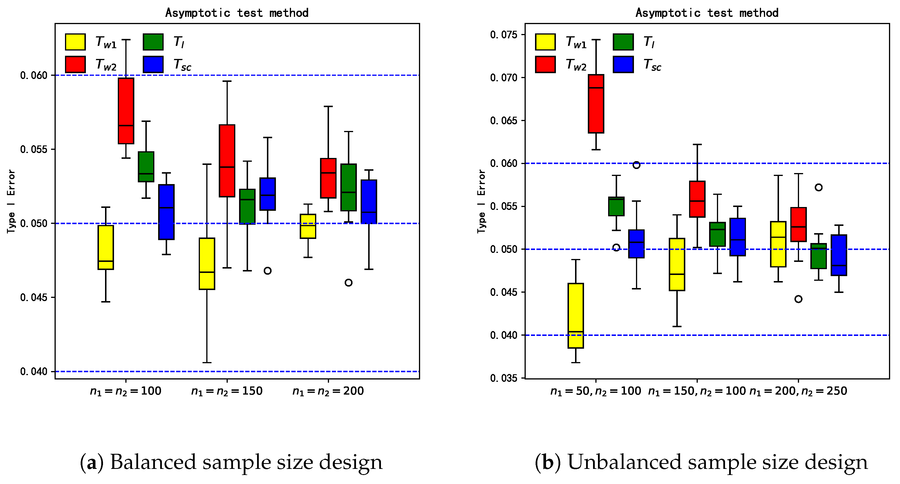
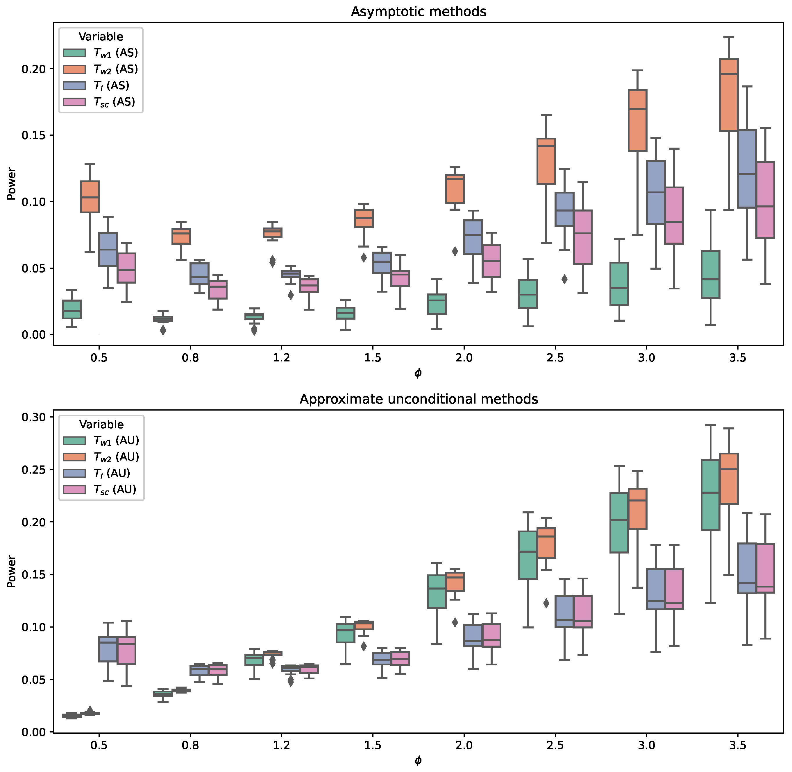
6.1. Empirical Study for Hypothesis Testing

In this section, we investigate the performance of various test procedures for the hypothesis testing H 0 : ϕ = 1 versus H 1 : ϕ 1 proposed in Section 3. We consider the following sample size designs: three balanced sample size designs, i.e., (i) moderate sample size n 1 = n 2 = 100 ; (ii) large sample size n 1 = n 2 = 150 ; (iii) large sample size n 1 = n 2 = 200 and three unbalanced sample size designs, i.e., (iv) moderate sample size n 1 = 50 and n 2 = 100 ; (v) large sample size n 1 = 150 and n 2 = 100 ; (vi) large sample size n 1 = 200 and n 2 = 250 . We do not consider the approximate unconditional methods for moderate to large sample sizes due to the extremely large number of possible values for m = ( n 00 ( 1 ) , n 10 ( 1 ) , n 01 ( 1 ) , n 11 ( 1 ) , n 00 ( 2 ) , n 10 ( 2 ) , n 01 ( 2 ) , n 11 ( 2 ) ) . However, the comparisons between the asymptotic (AS) and approximate unconditional (AU) methods are considered for small sample settings, including (vii) n 1 = n 2 = 10 and (viii) n 1 = n 2 = 15 . For each sample size design, we consider twelve different settings for the nuisance parameters ( π 00 ( 1 ) , π 11 ( 1 ) , π 00 ( 2 ) , π 11 ( 2 ) , π 10 ( 2 ) ) to investigate the performance of the various test procedures, and it is given in Table 2.
First, we examine the behavior of the actual test size, that is, the actual type I error rate of the testing procedure. For each sample size design and parameter setting, we generate M = 5000 observed samples for all test statistics. For the asymptotical test procedures, the empirical type I error rate for a given test T i ( i = w 1 , w 2 , l , s c ) , at significance level α = 0.05 for the settings under consideration, is simply estimated by (the number of rejections of H 0 by test T i at the α level)/M when ϕ = 1 . The results for moderate to large sample sizes are displayed in Figure 1. According to the Reviewer’s suggestion, we report the CMLEs and the MLEs of parameters π 00 ( 1 ) , π 11 ( 1 ) , π 01 ( 1 ) , π 10 ( 1 ) , π 00 ( 2 ) , π 11 ( 2 ) , π 01 ( 2 ) , π 10 ( 2 ) under small, moderate and large sample size designs via the online Supplemental Materials, respectively. Note that the CMLEs of parameters π 00 ( 1 ) , π 11 ( 1 ) , π 00 ( 2 ) and π 11 ( 2 ) are the same as their MLEs; we only report the results of parameters π 01 ( 1 ) , π 10 ( 1 ) , π 01 ( 2 ) and π 10 ( 2 ) . For the approximate unconditional test procedures, the actual type I error rate at the α level can be obtained by
m I { T i ( m ) ; α } [ exp ( l 2 ( m ; ϕ = 1 , π 10 ( 2 ) , π 00 ( 1 ) , π 11 ( 1 ) , π 00 ( 2 ) , π 11 ( 2 ) ) ) ] .
where I { T i ( m ) ; α } = 1 when the null hypothesis is rejected at α level, and I { T i ( m ) ; α } = 0 otherwise. According to Tang et al. [24], a test is liberal if its actual type I error rate exceeds 0.06, conservative if it falls below 0.04, and robust if it lies within the interval [0.04, 0.06] at 0.05 significant level. We summarize the results for n 1 = n 2 = 10 and are n 1 = n 2 = 15 in Table 3.
For the actual power performance of various test procedures, we consider the above sample size designs and the above nuisance parameter settings and ϕ 1 = 0.5 , 0.8 , 1.2 , 1.5 ( 0.5 ) 3.5 , where a ( b ) c denotes the value is from a to c with step size b. For the asymptotical test procedures, the empirical power for a given test T i ( i = w 1 ,   w 2 ,   l ,   s c ) , at significance level α = 0.05 for the settings under consideration, is estimated by (the number of rejections of H 0 by test T i at the α level)/M when ϕ = ϕ 1 . The simulation results for moderate to large sample sizes are displayed in Figure 2. For the approximate unconditional test procedures, the actual power at the α level can be obtained by
m I { T i ( m ) ; α } [ exp ( l 2 ( m ; ϕ = ϕ 1 , π 10 ( 2 ) , π 00 ( 1 ) , π 11 ( 1 ) , π 00 ( 2 ) , π 11 ( 2 ) ) ) ] .
We only reported the simulation results for the sample size design n 1 = n 2 = 15 by Figure 3 due to the space limitation. According to Figure 1 and Figure 2, we can observe that the asymptotical test procedures based on all test statistics perform well in the sense that the empirical type I errors are close to the nominal level under large sample sizes, and T w 2 has a slightly inflated type I error under some moderate sample sizes (e.g., n 1 = 50 , n 2 = 100 ). All test procedures have similar empirical powers under moderate to large sample sizes, except that T w 2 has slightly more power than the other test procedures. As expected, the empirical powers increase in all test procedures with the increase in the absolute difference between ϕ = 1 and ϕ 1 . When the sample size is large (e.g., sample sizes n 1 = 200 and n 2 = 250 ), four test statistics have similar performance; when the sample size increases, as expected, these four testing procedures are asymptotically equivalent. According to Table 3 and Figure 3, since the sample size is very small, the power performance was not satisfactory in some cases for both asymptotical and approximate unconditional test procedures. However, approximate unconditional procedures usually outperform the asymptotic test procedures in the sense that their empirical type I errors are closer to the nominal level and have higher powers under these small sample sizes. Therefore, when the sample size is small, the approximate unconditional test procedures based on these four test statistics are recommended for practical applications.

6.2. Empirical Study for Confidence Interval

In this section, we investigate the performance of these CIs for ϕ under various settings. The same parameter settings as those in Section 6.1 are considered. Four sample size designs were also considered, i.e., (i) n 1 = n 2 = 100 ; (ii) n 1 = n 2 = 200 ; (iii) n 1 = 150 and n 2 = 100 ; (iv) n 1 = 200 and n 2 = 250 . Under each sample size setting and each parameter combination, the empirical coverage probability, the empirical coverage width and the left and right non-coverage probability of the confidence interval are calculated by repeated simulation K = 5000 times. The three indices are calculated as follows:
(i)
Empirical coverage probability (ECP)
ECP = 1 K k = 1 K I { ϕ [ ϕ l ( m ( k ) ) , ϕ u ( m ( k ) ) ] } ,
where [ ϕ l ( m ( k ) ) , ϕ u ( m ( k ) ) ] is the confidence interval of ϕ at the kth replication, I ( · ) is the indicator function, m ( k ) = ( n 00 ( 1 ) , n 10 ( 1 ) , n 01 ( 1 ) , n 11 ( 1 ) , n 00 ( 2 ) , n 10 ( 2 ) , n 01 ( 2 ) , n 11 ( 2 ) ) ( k ) . Since the empirical coverage probability is defined as the proportion that the K confidence interval includes the true value of the interest parameter, then the closer the empirical coverage probability is to the nominal confidence level (e.g., 95%), the better the performance of the proposed method.
(ii)
Empirical coverage width (ECW)
ECW = 1 K k = 1 K { ϕ [ ϕ u ( m ( k ) ) ϕ l ( m ( k ) ) ] } .
It is obvious that a small empirical coverage width suggests a better confidence interval procedure if coverage can be maintained.
(iii)
Left and right non-coverage probability (LNCP, RNCP)
LNCP = 1 K k = 1 K I { ϕ < ϕ l ( m ( k ) ) } , RNCP = 1 K k = 1 K I { ϕ > ϕ u ( m ( k ) ) } .
Since left and right non-coverage probabilities are calculated as the proportions that the lower limit is above and the upper limit is below the true parameter value, respectively, so the confidence interval is regarded as having satisfactory interval location if the confidence interval procedure has equal left and right non-coverage probabilities.
Note that when n 01 ( 1 ) = 0 or n 10 ( 1 ) = 0 or n 01 ( 2 ) = 0 or n 10 ( 2 ) = 0 , the variance V a r ( c β ^ ) is undefined and its corresponding test statistics are undefined, so all Wald CIs are undefined. In this case, we use the commonly used adjustment for sparse data structures in contingency table analysis by adding 0.5 to each cell. For space limitations, we only present the simulation results for balanced sample sizes ( n 1 , n 2 ) = ( 100 , 100 ) , ( 200 , 200 ) and unbalanced sample sizes ( n 1 , n 2 ) = ( 150 , 100 ) in Table 4, Table 5 and Table 6, respectively. When the sample size is large, we can observe that (i) all CIs perform well in the sense that their empirical coverage probabilities are very close to the nominal confidence level; (ii) all CIs have satisfactory interval locations due to producing approximately symmetrical left-right non-coverage probabilities; (iii) similar interval widths for all CIs. However, when the sample size is not large (e.g., n 1 = n 2 = 100 ), CI w 2 based on the Wald statistic appears to perform poorly in some parameter settings, for example, A 2 , A 8 , A 9 and A 11 . Also, there is a slightly unbalance is observed in terms of left and right non-coverage probabilities and their expected confidence width is relatively wider than other CIs under those parameter sittings.

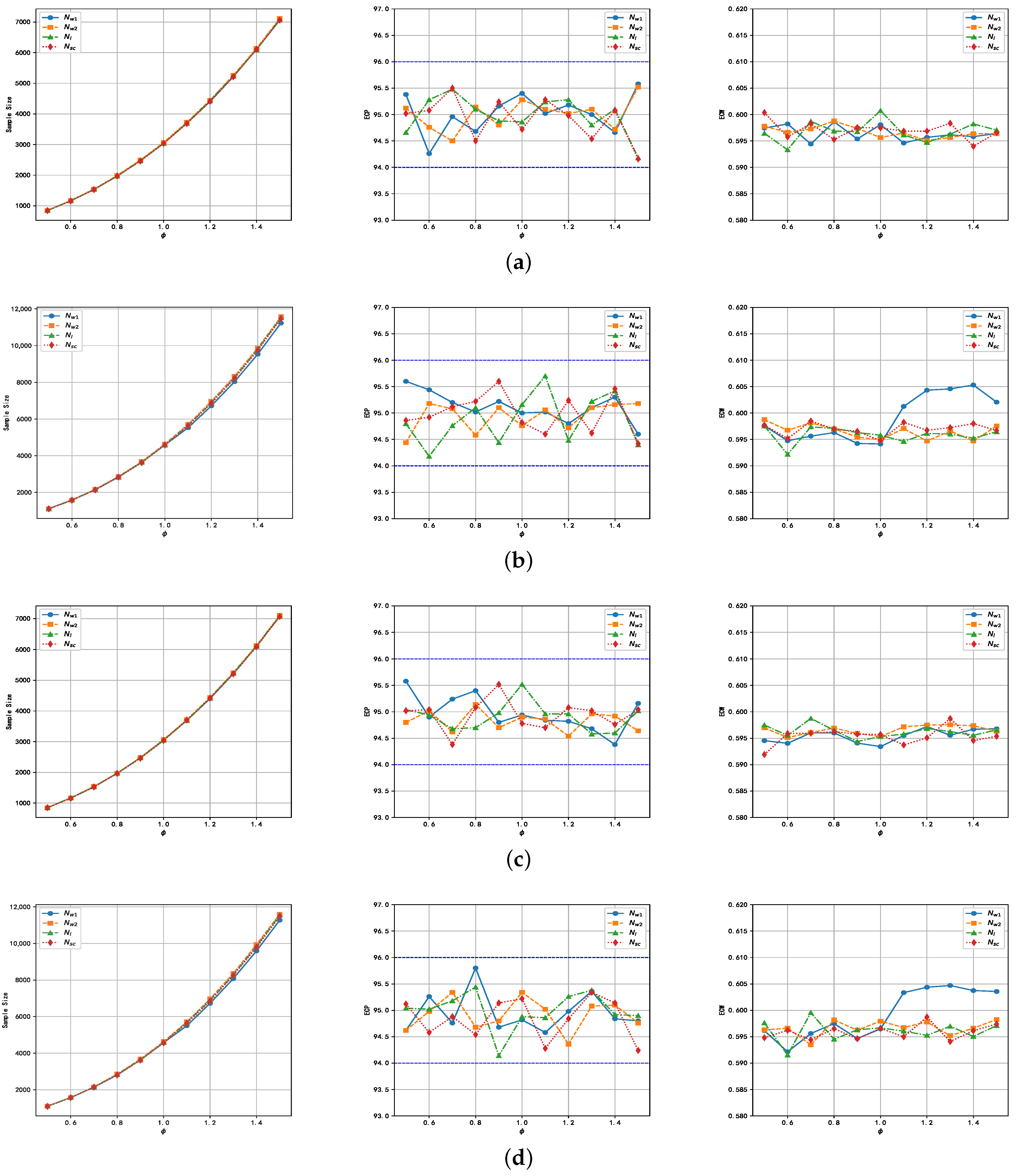
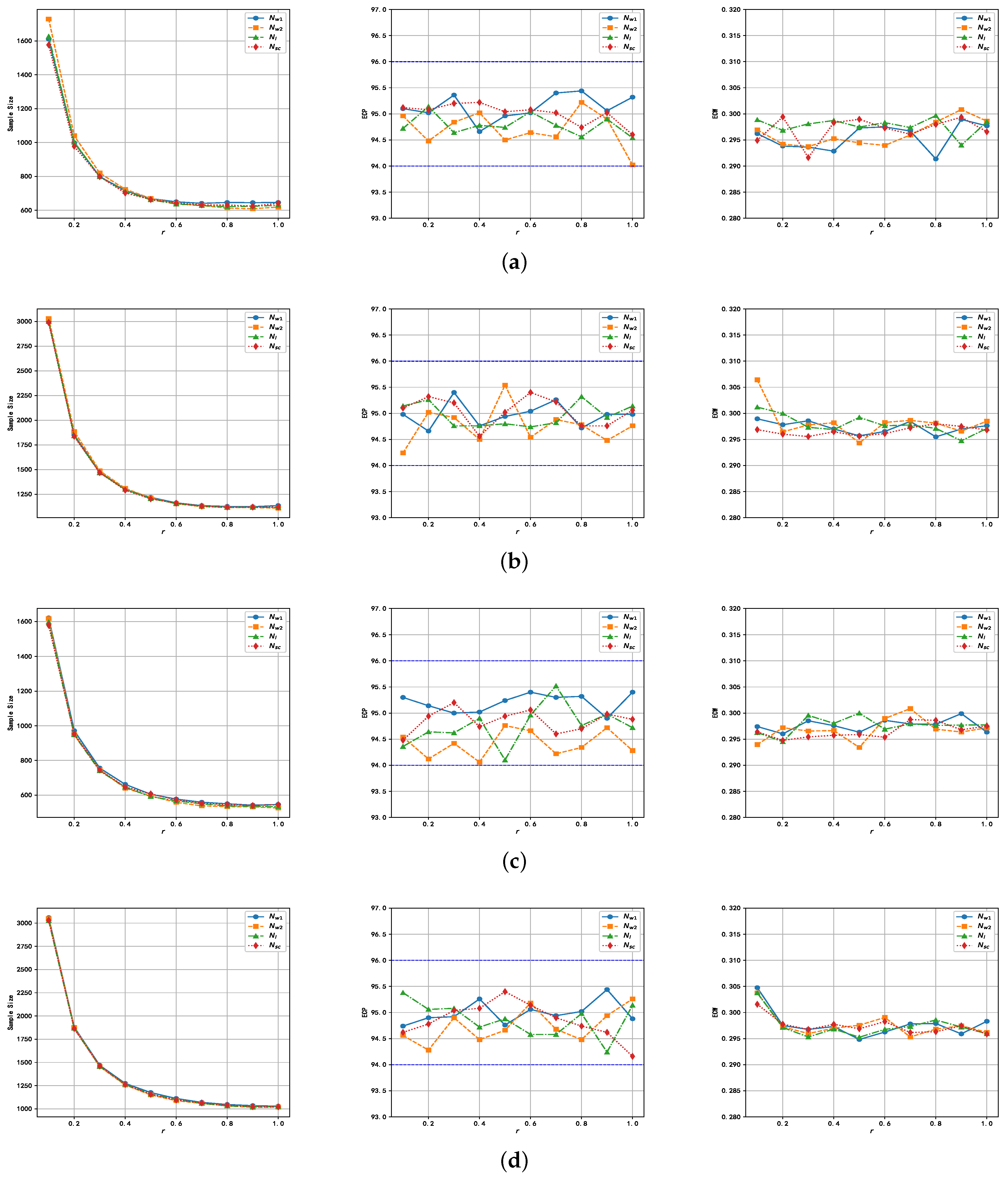
6.3. Empirical Study for Sample Size Determination

In this section, we investigate the performance of approximate sample size estimation methods that can control the width of a confidence interval within a pre-specified width at a given confidence level. For each setting of ϕ , π 10 ( 2 ) , π 00 ( 1 ) , π 11 ( 1 ) , π 00 ( 2 ) , π 11 ( 2 ) and r values, the approximate sample sizes N w 1 , N w 2 , N l and N s c are obtained via the algorithm proposed in Section 5. K = 5000 random samples are generated in the numerical algorithm. In order to investigate the accuracy of the estimated sample sizes, ECP and ECW of various CIs are calculated based on the estimated sample sizes. For given combinations of the parameters and a confidence interval C I i , sample size N i , where i = w 1 , w 2 , l , s c is determined. Based on the sample size, M = 5000 random samples for m are generated and confidence intervals are computed. The empirical coverage probabilities and empirical coverage widths based on the M = 5000 samples are obtained.
We consider different settings in our simulation study to study the effects of various factors. (i) To investigate the impact of ϕ , we consider various values of ϕ ranging from 0.5 to 1.5 with step size 0.1 , with π 00 ( 1 ) = 0.5 , π 11 ( 1 ) = 0.25 , π 00 ( 2 ) = 0.4 , π 11 ( 2 ) = 0.35 , half-width ω = 0.3 , and (a) r = 0.9 , π 10 ( 2 ) = 0.1 ; (b) r = 0.9 , π 10 ( 2 ) = 0.05 ; (c) r = 1 , π 10 ( 2 ) = 0.1 ; (d) r = 1 , π 10 ( 2 ) = 0.05 . The simulation results are available in Figure 4. (ii) To investigate the effect of r, we considered various r values ranging from 0.1 to 1 with step sizes 0.1, with π 00 ( 1 ) = 0.5 , π 11 ( 1 ) = 0.2 , π 00 ( 2 ) = 0.4 , π 11 ( 2 ) = 0.3 , half-width ω = 0.15 , and (a) ϕ = 0.2 , π 10 ( 2 ) = 0.15 ; (b) ϕ = 0.3 , π 10 ( 2 ) = 0.15 ; (c) ϕ = 0.2 , π 10 ( 2 ) = 0.1 ; (d) ϕ = 0.3 , π 10 ( 2 ) = 0.1 . The simulation results are available in Figure 5.
The simulation results indicate that (i) the required sample size increases with the increase in ϕ and decreases with the increase in r; (ii) based on the estimated sample sizes, the ECPs of all CIs are very close to the pre-specified confidence level, and the half-interval widths are also well controlled.

7. Real Example

7.1. Example of Two New Devices Delivering Salbutamol

To demonstrate the practicality and effectiveness of the proposed methods, we first consider an example of the AB/BA crossover test conducted by 3M Riker to compare the applicability of two new inhalation devices (A and B) in patients using standard inhalation devices to deliver salbutamol (Ezzet and Whitehead [13]). The response of the patient is either ‘yes’ or ‘no’, and neglecting the missing results of very few patients; the frequency of known reactions in patients is summarized in Table 7.
Assume that there is no significant difference between the preferences for device B and A, i.e., we are interested in the hypothesis testing: H 0 : ϕ = 1 versus H 1 : ϕ 1 . Based on the observed data, the MLE of the interest parameter ϕ is ϕ ^ = 0.1829 , and MLEs of π 01 ( 1 ) , π 10 ( 1 ) , π 01 ( 2 ) and π 10 ( 2 ) are given by π ^ 01 ( 1 ) = 0.1079 , π ^ 10 ( 1 ) = 0.2950 , π ^ 01 ( 2 ) = 0.2286 and π ^ 10 ( 2 ) = 0.1143 according to Euqation (3). The CMLEs of π 01 ( 1 ) , π 10 ( 1 ) , π 01 ( 2 ) and π 10 ( 2 ) are given by π ˜ 01 ( 1 ) = 0.1821 , π ˜ 10 ( 1 ) = 0.2208 , π ˜ 01 ( 2 ) = 0.1549 and π ˜ 10 ( 2 ) = 0.1879 according to Equation (7). The p-values of the asymptotic test procedures are based on T w 1 . T w 2 , T l and T s c are less than 0.001. The corresponding 95% confidence intervals for CI w 1 , CI w 2 , CI l and CI s c are [0.0788, 0.4248], [0.0710, 0.4041], [0.0767, 0.4163] and [0.0792, 0.4222], respectively. Therefore, we would reject the null hypothesis, i.e., there is a significant difference in patient preference rates between devices A and B, this conclusion is consistent with Li et al. [18]. Let ϕ = 0.2 , π 00 ( 1 ) = 0.4100 , π 11 ( 1 ) = 0.1871 , π 00 ( 2 ) = 0.3857 , π 11 ( 2 ) = 0.2714 , π 10 ( 2 ) = 0.1143 and r = 1 , we consider the sample size determination, and the desired sample sizes based on CI w 1 , CI w 2 , CI l and CI s c for controlling the interval width within 2 ω = 0.3 are N w 1 = 441 , N w 2 = 423 , N l = 429 , N s c = 438 , respectively. The corresponding empirical coverage probabilities are 95.36%, 94.80%, 95.08%, and 95.10%, respectively.

7.2. Example of Relieving Heartburn

Koch et al. [33] investigated an AB/BA crossover trial for comparing the efficacy of active drugs and placebo in relieving heartburn after two symptomatic meals (two meals corresponding to two cycles) from two centers. At each center, 30 patients participated in this trial, of which 15 were randomly assigned to the (A:P) sequence group (treated with active medication for heartburn in the first meal and placebo in the second meal), and the other 15 were assigned to the (P:A) sequence group (treated with placebo in the first meal and active medication in the second meal). The allocation of sequence groups adopts a double-blind method. The interval between each patient’s two periods (two meals) in the crossover design is several days, which is considered long enough to rule out any residual effects of treatment. The frequency data on whether or not the patient experienced relief within 15 min of the first dose of treatment in Center 2 are given in Table 8.
Suppose that there is no significant difference in the efficacy of active drugs and placebo, i.e., we consider the hypothesis testing H 0 : ϕ = 1 . With the data from Table 8, we have ϕ ^ = 0.0430 , the MLEs of π 01 ( 1 ) , π 10 ( 1 ) , π 01 ( 2 ) and π 10 ( 2 ) are given by π ^ 01 ( 1 ) = 0.0667 , π ^ 10 ( 1 ) = 0.4667 , π ^ 01 ( 2 ) = 0.6667 and π ^ 10 ( 2 ) = 0.2000 according to Euqation (3), and the CMLEs of π 01 ( 1 ) , π 10 ( 1 ) , π 01 ( 2 ) and π 10 ( 2 ) are given by π ˜ 01 ( 1 ) = 0.2794 , π ˜ 10 ( 1 ) = 0.2540 , π ˜ 01 ( 2 ) = 0.4540 and π ˜ 10 ( 2 ) = 0.4127 according to Equation (7). Since the sample size is very small, we consider both the asymptotic and approximate unconditional test procedures for the hypothesis testing H 0 : ϕ = 1 ; the asymptotic test p-values based on test statistics T w 1 . T w 2 , T l and T s c are 0.0127 , 0.0015 , 0.0047 , 0.0063 , and the corresponding approximate unconditional test p-values are 0.0048 , 0.0077 , 0.0040 , 0.0036 , respectively.
Obviously, the p-values of test procedures based on test statistics T w 1 , T w 2 , T l and T s c are less than 0.05, so these p-values strongly support a significant difference in heartburn relief between active treatment and placebo. Moreover, 95% CIs, i.e., CI w 1 , CI w 2 , CI l and CI s c are [0.0079, 0.5609], [0.0, 0.3747], [0.0054, 0.4597] and [0.0094, 0.5018], respectively. Let ϕ = 0.1 , π 00 ( 1 ) = 0.4412 , π 11 ( 1 ) = 0.0294 , π 00 ( 2 ) = 0.1471 , π 11 ( 2 ) = 0.0294 , π 10 ( 2 ) = 0.2059 and r = 1 , with the half interval width ω = 0.05 , the desired sample sizes are N w 1 = 605 , N w 2 = 587 , N l = 596 , N s c = 602 , respectively. The corresponding empirical coverage probabilities are 95.12%, 94.60%, 94.74%, and 95.26%, respectively.

8. Conclusions and Discussion

The equivalence test of odds ratio (OR) in an AB/BA crossover study with binary outcomes is considered in this article, two test procedures, including the asymptotical and approximate unconditional test procedures based on four test statistics, i.e., two Wald type test statistics, likelihood ratio test statistic and score test statistic are proposed to test the equivalence hypothesis. Four confidence intervals for the OR and the corresponding sample sizes, which can control the width of a confidence interval with a pre-specified confidence level, are developed. Simulation results indicate that the asymptotical test procedures based on four test statistics perform well when the sample size is not small, and the approximate test procedures can produce close to the nominal level even if the sample size is very small (e.g., n 1 = n 2 = 10 or n 1 = n 2 = 15 ). Confidence intervals derived from the score test statistic, likelihood ratio statistic, and Wald-type test statistics generally perform satisfactorily in terms of coverage. Take into account that in small sample sizes, the Wald CI based on T w 2 performs poorly under certain parameter settings. In general, sample size estimation methods can be recommended for practical applications in the sense that the empirical coverage probabilities are close to the pre-specified confidence level under the estimated sample sizes.
Under the assumption that there is no carryover effect or stage effect in an AB/BA crossover design, we considered the equivalence test, confidence interval and sample size determination based on OR for the treatment effects of two treatments. Python 5.4.1 codes that implement the proposed methodologies and calculations are available from the second author by request. However, the carryover effect and/or period effect may exist in some trials with binary outcomes. Therefore, statistical inference for the treatment effects in the crossover trials with carryover effect and/or period effect will be considered in the future. In this article, we provide some estimation methods for sample size determination which can control the width of a confidence interval, but we do not take the cost into account for the sample size estimation, it also may be the interest topic in the future research.

Supplementary Materials

The following supporting information can be downloaded at: https://www.mdpi.com/article/10.3390/axioms14080582/s1.

Author Contributions

Formal analysis, X.-Q.Y.; Funding acquisition, S.-F.Q.; Methodology, S.-F.Q., X.-Q.Y. and W.-Y.P.; Project administration, W.-Y.P.; Supervision, S.-F.Q.; Writing—original draft, X.-Q.Y.; Writing—review and editing, S.-F.Q. and W.-Y.P. All authors have read and agreed to the published version of the manuscript.

Funding

The work of Dr. Qiu was sponsored by Science and Technology Research Program of Chongqing Municipal Education Commission (Grant No. KJZD-K202201101), the Natural Science Foundation of Chongqing, China (Grant No. CSTB2024NSCQ-LZX0136), and the National Natural Science Foundation of China (Grant No. 11871124).

Data Availability Statement

No new data were generated during this study. All real examples are publicly available and cited appropriately.

Conflicts of Interest

The authors declare no conflicts of interest.

Appendix A. Derivation of the CMLE π ˜ 10 ( 2 ) of π 10 ( 2 ) Given ϕ

The CMLE π ˜ 10 ( 2 ) of π 10 ( 2 ) is the root of the following quadratic equation
A ( π 10 ( 2 ) ) 2 + B π 10 ( 2 ) + C = 0 .
where A = ( ϕ 1 ) ( n 01 ( 2 ) + n 10 ( 2 ) ) , B = m 2 ( n 10 ( 2 ) n 01 ( 1 ) ) m 2 ( n 01 ( 2 ) + n 10 ( 1 ) + 2 n 10 ( 2 ) ) , C = ϕ ( n 10 ( 1 ) + n 10 ( 2 ) ) m 2 2 with m 1 = ( n 01 ( 1 ) + n 10 ( 1 ) ) / n 1 , m 2 = ( n 01 ( 2 ) + n 10 ( 2 ) ) / n 2 . Therefore, we have
B 2 4 A C = m 2 2 [ ( n 10 ( 2 ) n 01 ( 1 ) ) ϕ ( n 01 ( 2 ) + n 10 ( 1 ) + n 10 ( 2 ) + n 10 ( 2 ) ) ] 2 4 ϕ ( ϕ 1 ) ( n 01 ( 2 ) + n 10 ( 2 ) ) ( n 10 ( 1 ) + n 10 ( 2 ) ) m 2 2 = m 2 2 { [ ( n 10 ( 2 ) n 01 ( 1 ) ) 2 + ϕ 2 ( n 01 ( 2 ) + n 10 ( 1 ) + n 10 ( 2 ) + n 10 ( 2 ) ) 2 2 ( n 10 ( 2 ) n 01 ( 1 ) ) ( n 01 ( 2 ) + n 10 ( 1 ) + n 10 ( 2 ) + n 10 ( 2 ) ) ϕ ] 4 ( n 01 ( 2 ) + n 10 ( 2 ) ) ( n 10 ( 1 ) + n 10 ( 2 ) ) ϕ 2 + 4 ( n 01 ( 2 ) + n 10 ( 2 ) ) ( n 10 ( 1 ) + n 10 ( 2 ) ) ϕ } = m 2 2 { ϕ 2 ( n 01 ( 2 ) n 10 ( 1 ) ) 2 + 2 ϕ [ ( n 10 ( 1 ) + n 10 ( 2 ) ) ( n 01 ( 2 ) + n 01 ( 1 ) ) + ( n 01 ( 2 ) + n 10 ( 2 ) ) ( n 10 ( 1 ) + n 01 ( 1 ) ) ] + ( n 10 ( 2 ) n 01 ( 1 ) ) 2 }
Obviously, B 2 4 A C is aways not less than 0, which indicates that the quadratic equation about π 10 ( 2 ) , i.e., A ( π 10 ( 2 ) ) 2 + B π 10 ( 2 ) + C = 0 must have roots. Moreover, it is easily seen that 4 A C = ϕ ( ϕ 1 ) ( n 01 ( 2 ) + n 10 ( 2 ) ) ( n 10 ( 1 ) + n 10 ( 2 ) ) m 2 2 , so | B | > B 2 4 A C if ϕ > 1 , and | B | < B 2 4 A C if ϕ < 1 .
Case 1:  ϕ > 1
In this case, A > 0 , B < 0 and B B 2 4 A C > 0 , the quadratic Equation (A1) has two positive roots:
( B B 2 4 A C ) / ( 2 A ) and ( B + B 2 4 A C ) / ( 2 A ) .
Due to 0 π 00 ( 2 ) , π 01 ( 2 ) , π 10 ( 2 ) , π 11 ( 2 ) 1 and π 00 ( 2 ) + π 01 ( 2 ) + π 10 ( 2 ) + π 11 ( 2 ) = 1 , the CMLE π ˜ 10 ( 2 ) of π 10 ( 2 ) should be the smaller positive root, i.e., π ˜ 10 ( 2 ) = ( B B 2 4 A C ) / ( 2 A ) .
Case 2:  ϕ < 1
In this case, since A < 0 , then ( B B 2 4 A C ) < 0 and ( B + B 2 4 A C ) > 0 . The quadratic Equation (A1) has a positive root ( B B 2 4 A C ) / ( 2 A ) and a negative root ( B + B 2 4 A C ) / ( 2 A ) )). Due to π 10 ( 2 ) > 0 , then the CMLE π ˜ 10 ( 2 ) of π 10 ( 2 ) should be π ˜ 10 ( 2 ) = ( B + B 2 4 A C ) / ( 2 A ) .
To sum up, when A 0 , the CMLE π ˜ 10 ( 2 ) of π 10 ( 2 ) is given by π ˜ 10 ( 2 ) = ( B B 2 4 A C ) / ( 2 A ) . When A = 0 , Equation (A1) becomes B π 10 ( 2 ) + C = 0 , it has a single root π ˜ 10 ( 2 ) = C / B .

Appendix B. Derivation of the Asymptotical Distribution of the Test Statistic Tw1 (Tw2)

Let π ( 1 ) = ( π 01 ( 1 ) , π 10 ( 1 ) ) , π ( 2 ) = ( π 01 ( 2 ) , π 10 ( 2 ) ) , the corresponding MLEs of π ( 1 ) and π ( 2 ) are π ^ ( 1 ) and π ^ ( 2 ) , respectively. Under the regularity conditions π 00 ( 1 ) , π 10 ( 1 ) , π 01 ( 1 ) , π 11 ( 1 ) , π 00 ( 2 ) , π 10 ( 2 ) , π 01 ( 2 ) , π 11 ( 2 ) > 0 , the MLEs π ^ ( 1 ) and π ^ ( 2 ) of the multinomial distribution parameter vectors π ( 1 ) and π ( 2 ) are asymptotically distributed as the normal distributions when min { n 1 , n 2 } , that is
n i ( π ^ ( i ) π ( i ) ) d N 2 ( 0 , Σ π ( i ) ) , Σ π ( i ) = d i a g ( π ( i ) ) π ( i ) π ( i ) , i = 1 , 2 .
Let β ( 1 ) = ( log π 01 ( 1 ) , log π 10 ( 1 ) ) , β ( 2 ) = ( log π 01 ( 2 ) , log π 10 ( 2 ) ) . According to the delta method, we have
n i ( β ^ ( i ) β ( i ) ) d N 2 ( 0 , Σ β ( i ) ) , Σ β ( i ) = 1 π 01 ( i ) π 01 ( i ) 1 1 1 π 10 ( i ) π 10 ( i ) , i = 1 , 2 .
Therefore, we have
β ^ β = β ^ ( 1 ) β ^ ( 2 ) β ( 1 ) β ( 2 ) d N 4 ( 0 4 × 1 , Σ ) , Σ = 1 n 1 Σ β ( 1 ) 0 2 × 2 0 2 × 2 1 n 2 Σ β ( 2 ) .
Thus,
c β ^ c c β c d N ( 0 , c Σ c )
Since Σ ^ π ( i ) = d i a g ( π ^ ( i ) ) π ^ ( i ) ( π ^ ( i ) ) is the consistent estimator of Σ π ( i ) for i = 1 , 2 , and g ( x ) = log ( x ) is a continuously differentiable function, then the estimator of Σ , which is obtained by replacing the parameters (i.e., π 01 ( 1 ) , π 10 ( 1 ) , π 01 ( 2 ) , π 10 ( 2 ) ) with their MLEs or their constrained MLEs under H 0 : ϕ = 1 , is the consistent estimator of Σ . Therefore, under the null hypothesis H 0 : c β = 0 , we have
Z 1 = ( c β ^ c ) / c Σ ^ c d N ( 0 , 1 ) , Z 2 = ( c β ^ c ) / c Σ ˜ c d N ( 0 , 1 ) .
When min { n 1 , n 2 } . Then T w 1 = Z 1 2 and T w 2 = Z 2 2 are asymptotically distributed as the χ 2 distribution with one degree of freedom.

Appendix C. Derivation of Score Test Statistic

Differentiating l 2 ( ϕ , π 00 ( 1 ) , π 11 ( 1 ) , π 00 ( 2 ) , π 11 ( 2 ) , π 10 ( 2 ) ) respect to ϕ , π 00 ( 1 ) , π 11 ( 1 ) , π 00 ( 2 ) , π 11 ( 2 ) , and π 10 ( 2 ) yields
l 2 ϕ = n 01 ( 1 ) ϕ ( M 2 π 10 ( 2 ) ) ( n 01 ( 1 ) + n 10 ( 1 ) ) π 10 ( 2 ) + ϕ ( M 2 π 10 ( 2 ) ) ,
l 2 π 10 ( 2 ) = n 01 ( 1 ) + n 01 ( 2 ) M 2 π 10 ( 2 ) ( 1 ϕ ) ( n 01 ( 1 ) + n 10 ( 1 ) ) π 10 ( 2 ) + ϕ ( M 2 π 10 ( 2 ) ) + n 10 ( 1 ) + n 10 ( 2 ) π 10 ( 2 ) ,
l 2 π 00 ( 1 ) = n 00 ( 1 ) π 00 ( 1 ) n 01 ( 1 ) + n 10 ( 1 ) M 1 ,
l 2 π 11 ( 1 ) = n 11 ( 1 ) π 11 ( 1 ) n 01 ( 1 ) + n 10 ( 1 ) M 1 ,
l 2 π 00 ( 2 ) = n 00 ( 2 ) π 00 ( 2 ) n 01 ( 1 ) + n 01 ( 2 ) M 2 π 10 ( 2 ) + ϕ ( n 10 ( 1 ) + n 01 ( 1 ) ) π 10 ( 2 ) + ϕ ( M 2 π 10 ( 2 ) ) , and l 2 π 11 ( 2 ) = n 11 ( 2 ) π 11 ( 2 ) n 01 ( 1 ) + n 01 ( 2 ) M 2 π 10 ( 2 ) + ϕ ( n 10 ( 1 ) + n 01 ( 1 ) ) π 10 ( 2 ) + ϕ ( M 2 π 10 ( 2 ) ) .
Differentiating l 2 ϕ , l 2 π 10 ( 2 ) , l 2 π 00 ( 1 ) , l 2 π 11 ( 1 ) , l 2 π 00 ( 2 ) , l 2 π 11 ( 2 ) with respect to ϕ , π 00 ( 1 ) , π 11 ( 1 ) , π 00 ( 2 ) , π 11 ( 2 ) , and π 10 ( 2 ) , respectively, and yields
2 l 2 ϕ ϕ = n 01 ( 1 ) ϕ 2 + ( M 2 π 10 ( 2 ) ) 2 ( n 01 ( 1 ) + n 10 ( 1 ) ) ( π 10 ( 2 ) + ϕ ( M 2 π 10 ( 2 ) ) ) 2 ,
2 l 2 ϕ π 10 ( 2 ) = 2 l 2 π 10 ( 2 ) ϕ = M 2 ( n 01 ( 1 ) + n 10 ( 1 ) ) ( π 10 ( 2 ) + ϕ ( M 2 π 10 ( 2 ) ) ) 2 ,
2 l 2 ϕ π 00 ( 2 ) = 2 l 2 π 00 ( 2 ) ϕ = 2 l 2 ϕ π 11 ( 2 ) = 2 l 2 π 11 ( 2 ) ϕ = ( n 01 ( 1 ) + n 10 ( 1 ) ) π 10 ( 2 ) ( π 10 ( 2 ) + ϕ ( M 2 π 10 ( 2 ) ) ) 2 ,
2 l 2 π 10 ( 2 ) π 10 ( 2 ) = ( n 01 ( 1 ) + n 01 ( 2 ) ) ( M 2 π 10 ( 2 ) ) 2 + ( 1 ϕ ) 2 ( n 01 ( 1 ) + n 10 ( 2 ) ) ( π 10 ( 2 ) + ϕ ( M 2 π 10 ( 2 ) ) ) 2 n 10 ( 1 ) + n 10 ( 2 ) ( π 10 ( 2 ) ) 2 ,
2 l 2 π 10 ( 2 ) π 00 ( 2 ) = 2 l 2 π 00 ( 2 ) π 10 ( 2 ) = 2 l 2 π 10 ( 2 ) π 11 ( 2 ) = 2 l 2 π 11 ( 2 ) π 10 ( 2 ) = n 01 ( 2 ) + n 01 ( 1 ) ( M 2 π 10 ( 2 ) ) 2 ( 1 ϕ ) ϕ ( n 01 ( 1 ) + n 10 ( 1 ) ) ( π 10 ( 2 ) + ϕ ( M 2 π 10 ( 2 ) ) ) 2 ,
2 l 2 ϕ π 11 ( 1 ) = 2 l 2 ϕ π 00 ( 1 ) = 2 l 2 π 10 ( 2 ) π 11 ( 1 ) = 2 l 2 π 10 ( 2 ) π 00 ( 1 ) = 0 ,
2 l 2 π 00 ( 1 ) π 00 ( 1 ) = n 00 ( 1 ) ( π 00 ( 1 ) ) 2 n 01 ( 1 ) + n 10 ( 1 ) M 1 2 ,
2 l 2 π 00 ( 1 ) π 11 ( 1 ) = 2 l 2 π 11 ( 1 ) π 00 ( 1 ) = n 01 ( 1 ) + n 10 ( 1 ) M 1 2 ,
2 l 2 π 00 ( 1 ) ϕ = 2 l 2 π 00 ( 1 ) π 10 ( 2 ) = 2 l 2 π 00 ( 1 ) π 00 ( 2 ) = 2 l 2 π 00 ( 1 ) π 11 ( 2 ) = 0 ,
2 l 2 π 11 ( 1 ) π 11 ( 1 ) = n 11 ( 1 ) ( π 11 ( 1 ) ) 2 n 01 ( 1 ) + n 10 ( 1 ) M 1 2 ,
2 l 2 π 11 ( 1 ) ϕ = 2 l 2 π 11 ( 1 ) π 10 ( 2 ) = 2 l 2 π 11 ( 1 ) π 11 ( 2 ) = 2 l 2 π 11 ( 1 ) π 00 ( 2 ) = 0 ,
2 l 2 π 00 ( 2 ) π 00 ( 2 ) = n 00 ( 2 ) ( π 00 ( 2 ) ) 2 n 01 ( 1 ) + n 01 ( 2 ) ( M 2 π 10 ( 2 ) ) 2 + ϕ 2 ( n 10 ( 1 ) + n 01 ( 1 ) ) ( π 10 ( 2 ) + ϕ ( M 2 π 10 ( 2 ) ) ) 2 ,
2 l 2 π 00 ( 2 ) π 11 ( 2 ) = 2 l 2 π 11 ( 2 ) π 00 ( 2 ) = n 01 ( 1 ) + n 01 ( 2 ) ( M 2 π 10 ( 2 ) ) + ϕ 2 ( n 01 ( 1 ) + n 10 ( 1 ) ) ( π 10 ( 2 ) + ϕ ( M 2 π 10 ( 2 ) ) ) 2 ,
2 l 2 π 11 ( 2 ) π 11 ( 2 ) = n 11 ( 2 ) ( π 11 ( 2 ) ) 2 n 01 ( 1 ) + n 01 ( 2 ) ( M 2 π 10 ( 2 ) ) 2 + ϕ 2 ( n 10 ( 1 ) + n 01 ( 1 ) ) ( π 10 ( 2 ) + ϕ ( M 2 π 10 ( 2 ) ) ) 2 ,
2 l 2 π 00 ( 2 ) π 00 ( 1 ) = 2 l 2 π 00 ( 2 ) π 11 ( 1 ) = 2 l 2 π 11 ( 2 ) π 00 ( 1 ) = 2 l 2 π 11 ( 2 ) π 11 ( 1 ) = 0 .
Let Q 1 = π 10 ( 2 ) + ϕ ( M 2 π 10 ( 2 ) ) = π 10 ( 2 ) + ϕ π 01 ( 2 ) ; Q 2 = n 1 ( π 01 ( 1 ) + π 10 ( 1 ) ) ; Q 3 = ( n 1 π 01 ( 1 ) + n 2 π 01 ( 2 ) ) / ( π 01 ( 2 ) ) 2 . Next, we have
I ϕ ϕ = E ( 2 l 2 ϕ ϕ ) = n 1 π 01 ( 1 ) ϕ 2 Q 2 ( π 01 ( 2 ) ) 2 Q 1 2 ,
I ϕ π 10 ( 2 ) = I π 10 ( 2 ) ϕ = E ( 2 l 2 ϕ π 10 ( 2 ) ) = Q 2 M 2 Q 1 2 ,
I ϕ π 00 ( 2 ) = I π 00 ( 2 ) ϕ = E ( 2 l 2 π 00 ( 2 ) ϕ ) = Q 2 π 10 ( 2 ) Q 1 2 = I ϕ π 11 ( 2 ) = I π 11 ( 2 ) ϕ ,
I π 10 ( 2 ) π 10 ( 2 ) = E ( 2 l 2 π 10 ( 2 ) π 10 ( 2 ) ) = n 1 π 10 ( 1 ) + n 2 π 10 ( 2 ) ( π 10 ( 2 ) ) 2 ( 1 ϕ ) 2 Q 2 Q 1 2 + Q 3 ,
I π 10 ( 2 ) π 00 ( 2 ) = I π 00 ( 2 ) π 10 ( 2 ) = E ( 2 l 2 π 10 ( 2 ) π 00 ( 2 ) ) = Q 3 + ϕ ( 1 ϕ ) Q 2 Q 1 2 = I π 10 ( 2 ) π 11 ( 2 ) = I π 11 ( 2 ) π 10 ( 2 ) ,
I π 00 ( 1 ) π 00 ( 1 ) = E ( 2 l 2 π 00 ( 1 ) π 00 ( 1 ) ) = n 1 π 00 ( 1 ) + Q 2 M 1 2 ,
I π 00 ( 1 ) π 11 ( 1 ) = I π 11 ( 1 ) π 00 ( 1 ) = E ( 2 l 2 π 00 ( 1 ) π 11 ( 1 ) ) = Q 2 M 1 2 ,
I π 11 ( 1 ) π 11 ( 1 ) = E ( 2 l 2 π 11 ( 1 ) π 11 ( 1 ) ) = n 1 π 11 ( 1 ) + Q 2 M 1 2 ,
I π 00 ( 2 ) π 00 ( 2 ) = E ( 2 l 2 π 00 ( 2 ) π 00 ( 2 ) ) = n 2 π 00 ( 2 ) + Q 3 Q 2 ϕ 2 Q 1 2 ,
I π 00 ( 2 ) π 11 ( 2 ) = I π 11 ( 2 ) π 00 ( 2 ) = E ( 2 l 2 π 00 ( 2 ) π 11 ( 2 ) ) = Q 3 Q 2 ϕ 2 Q 1 2 ,
I π 11 ( 2 ) π 11 ( 2 ) = E ( 2 l 2 π 11 ( 2 ) π 11 ( 2 ) ) = n 2 π 11 ( 2 ) + Q 3 Q 2 ϕ 2 Q 1 2 ,
I ϕ π 00 ( 1 ) = I ϕ π 11 ( 1 ) = I π 00 ( 1 ) ϕ = I π 11 ( 1 ) ϕ = I π 10 ( 2 ) π 00 ( 1 ) = I π 10 ( 2 ) π 11 ( 1 ) = I π 00 ( 1 ) π 10 ( 2 ) = I π 00 ( 1 ) π 00 ( 2 ) = I π 00 ( 1 ) π 11 ( 2 ) ,
I π 11 ( 1 ) π 10 ( 2 ) = I π 11 ( 1 ) π 00 ( 2 ) = I π 11 ( 2 ) π 11 ( 2 ) = I π 00 ( 2 ) π 00 ( 1 ) = I π 00 ( 2 ) π 11 ( 1 ) = I π 11 ( 2 ) π 00 ( 1 ) = I π 11 ( 2 ) π 11 ( 1 ) = 0 .
Thus, the Fisher information matrix is given by
I ( ϕ , π 10 ( 2 ) , π 00 ( 1 ) , π 11 ( 1 ) , π 00 ( 2 ) , π 11 ( 2 ) ) = I ϕ ϕ I ϕ π 10 ( 2 ) I ϕ π 00 ( 1 ) I ϕ π 11 ( 1 ) I ϕ π 00 ( 2 ) I ϕ π 11 ( 2 ) I π 10 ( 2 ) ϕ I π 10 ( 2 ) π 10 ( 2 ) I π 10 ( 2 ) π 00 ( 1 ) I π 10 ( 2 ) π 11 ( 1 ) I π 10 ( 2 ) π 00 ( 2 ) I π 10 ( 2 ) π 11 ( 2 ) I π 00 ( 1 ) ϕ I π 00 ( 1 ) π 10 ( 2 ) I π 00 ( 1 ) π 00 ( 1 ) I π 00 ( 1 ) π 11 ( 1 ) I π 00 ( 1 ) π 00 ( 2 ) I π 00 ( 1 ) π 11 ( 2 ) I π 11 ( 1 ) ϕ I π 11 ( 1 ) π 10 ( 2 ) I π 11 ( 1 ) π 00 ( 1 ) I π 11 ( 1 ) π 11 ( 1 ) I π 11 ( 1 ) π 00 ( 2 ) I π 11 ( 1 ) π 00 ( 2 ) I π 00 ( 2 ) ϕ I π 00 ( 2 ) π 10 ( 2 ) I π 00 ( 2 ) π 00 ( 1 ) I π 00 ( 2 ) π 11 ( 1 ) I π 00 ( 2 ) π 00 ( 2 ) I π 00 ( 2 ) π 11 ( 2 ) I π 11 ( 2 ) ϕ I π 11 ( 2 ) π 10 ( 2 ) I π 11 ( 2 ) π 00 ( 1 ) I π 11 ( 2 ) π 11 ( 1 ) I π 11 ( 2 ) π 00 ( 2 ) I π 11 ( 2 ) π 11 ( 2 )
Under H 0 : ϕ = 1 , we have the Fisher information matrix
I 0 ( ϕ , π 10 ( 2 ) , π 00 ( 1 ) , π 11 ( 1 ) , π 00 ( 2 ) , π 11 ( 2 ) ) = I ϕ ϕ 0 I ϕ π 10 ( 2 ) 0 0 0 I ϕ π 00 ( 2 ) 0 I ϕ π 11 ( 2 ) 0 I π 10 ( 2 ) ϕ 0 I π 10 ( 2 ) π 10 ( 2 ) 0 0 0 I π 10 ( 2 ) π 00 ( 2 ) 0 I π 10 ( 2 ) π 11 ( 2 ) 0 0 0 I π 00 ( 1 ) π 00 ( 1 ) 0 I π 00 ( 1 ) π 11 ( 1 ) 0 0 0 0 0 I π 11 ( 1 ) π 00 ( 1 ) 0 I π 11 ( 1 ) π 11 ( 1 ) 0 0 0 I π 00 ( 2 ) ϕ 0 I π 00 ( 2 ) π 10 ( 2 ) 0 0 0 I π 00 ( 2 ) π 00 ( 2 ) 0 I π 00 ( 2 ) π 11 ( 2 ) 0 I π 11 ( 2 ) ϕ 0 I π 11 ( 2 ) π 10 ( 2 ) 0 0 0 I π 11 ( 2 ) π 00 ( 2 ) 0 I π 11 ( 2 ) π 11 ( 2 ) 0
and its inverse matrix is given by
I 0 1 ( ϕ , π 10 ( 2 ) , π 00 ( 1 ) , π 11 ( 1 ) , π 00 ( 2 ) , π 11 ( 2 ) ) = I 11 I 12 I 13 I 14 I 15 I 16 I 21 I 22 I 23 I 24 I 25 I 26 I 31 I 32 I 33 I 34 I 35 I 36 I 41 I 42 I 43 I 44 I 45 I 46 I 51 I 52 I 53 I 54 I 55 I 56 I 61 I 62 I 63 I 64 I 65 I 66
where
I 11 = I ϕ ϕ 0 ( I ϕ π 10 ( 2 ) 0 0 0 I ϕ π 00 ( 2 ) 0 I ϕ π 11 ( 2 ) 0 ) I π 10 ( 2 ) π 10 ( 2 ) 0 0 0 I π 10 ( 2 ) π 00 ( 2 ) 0 I π 10 ( 2 ) π 11 ( 2 ) 0 0 I π 00 ( 1 ) π 00 ( 1 ) 0 I π 00 ( 1 ) π 11 ( 1 ) 0 0 0 0 I π 11 ( 1 ) π 00 ( 1 ) 0 I π 11 ( 1 ) π 11 ( 1 ) 0 0 0 I π 00 ( 2 ) π 10 ( 2 ) 0 0 0 I π 00 ( 2 ) π 00 ( 2 ) 0 I π 00 ( 2 ) π 11 ( 2 ) 0 I π 11 ( 2 ) π 10 ( 2 ) 0 0 0 I π 11 ( 2 ) π 00 ( 2 ) 0 I π 11 ( 2 ) π 11 ( 2 ) 0 1 I π 10 ( 2 ) ϕ 0 0 0 I π 00 ( 2 ) ϕ 0 I π 11 ( 2 ) ϕ 0 1

References

  1. Hills, M.; Armitage, P. The two-period cross-over clinical trial. Br. J. Pharmacol. 1979, 8, 7. [Google Scholar] [CrossRef] [PubMed]
  2. Fleiss, J.L. The Design and Analysis of Clinical Experiments; John Wiley & Sons: New York, NY, USA, 1986. [Google Scholar]
  3. Senn, S.J. Cross-Over Trials in Clinical Research, 2nd ed.; John Wiley & Sons, Ltd.: Chichester, UK, 2002. [Google Scholar]
  4. Sever, P.S.; Poulter, N.R.; Bulpitt, C.J. Double-blind crossover versus parallel groups in hypertension. Am. Heart J. 1989, 117, 735–739. [Google Scholar] [CrossRef] [PubMed]
  5. Ménard, J.; Serrurier, D.; Bautier, P.; Plouin, P.-F.; Alexandre, J.-M.; Corvol, P. Crossover design to test antihypertensive drugs with self-recorded blood pressure. Hypertension 1988, 117, 153–159. [Google Scholar] [CrossRef] [PubMed]
  6. Grenet, G.; Blanc, C.; Bardel, C.; Francillard, I.; Combret, S.; Pivot, X.; Roy, P. Comparison of crossover and parallel-group designs for the identification of a binary predictive biomarker of the treatment effect. Basic Clin. Physiol. Pharmacol. 2020, 126, 59–64. [Google Scholar] [CrossRef]
  7. Jones, B.; Kenward, M.G. Design and Analysis of Cross-Over Trials; Chapman and Hall: London, UK, 1989. [Google Scholar]
  8. Senn, S. Cross-over trials in Statistics in Medicine: The first ‘25’ years. Stat. Med. 2006, 25, 3430–3442. [Google Scholar] [CrossRef]
  9. Mills, E.J.; Chan, A.W.; Wu, P.; Vail, A.; Guyatt, G.H.; Altman, D.G. Design, Analysis, and Presentation of Crossover Trials. Trials 2009, 10, 27. [Google Scholar] [CrossRef]
  10. Fava, G.M.; Patel, H.I. A Survey of Crossover Designs Used in Industry. Unpublished manuscript. 1986. [Google Scholar]
  11. Jones, B.; Kenward, M.G. Design and Analysis of Cross-Over Trials, 3rd ed.; Chapman & Hall/CRC, Taylor & Francis: Boca Raton, FL, USA, 2014. [Google Scholar]
  12. Kershner, R.P.; Federer, W.T. Two-treatment crossover designs for estimating a variety of effects. J. Am. Stat. Assoc. 1981, 76, 612–619. [Google Scholar] [CrossRef]
  13. Ezzet, F.; Whitehead, J. A random effects model for binary data from crossover clinical trials. J. R. Stat. Soc. C-Appl. 1992, 41, 117–126. [Google Scholar] [CrossRef]
  14. Becker, M.P.; Balagtas, C.C. Marginal modeling of binary cross-over data. Biometrics 1993, 49, 997–1009. [Google Scholar] [CrossRef]
  15. Jaki, T.; Pallmann, P. Estimation in AB/BA crossover trials with application to bioequivalence studies with incomplete and complete data designs. Stat. Med. 2013, 32, 5469–5483. [Google Scholar] [CrossRef]
  16. Lui, K.J.; Chang, K.C. Hypothesis testing and estimation in ordinal data under a simple crossover design. J. Biopharm. Stat. 2012, 22, 1137–1147. [Google Scholar] [CrossRef]
  17. Lui, K.J. Crossover Designs: Testing, Estimation, and Sample Size; John Wiley & Sons, Ltd.: Chichester, UK, 2016. [Google Scholar]
  18. Li, X.; Li, H.; Jin, M.; Goldberg, J.D. Likelihood ratio and score tests to test the non-inferiority (or equivalence) of the odds ratio in a crossover study with binary outcomes. Stat. Med. 2016, 35, 3471–3481. [Google Scholar] [CrossRef]
  19. Lui, K.J. Estimation of the treatment effect under an incomplete block crossover design in binary data-a conditional likelihood approach. Stat. Methods Med. Res. 2017, 26, 2197–2209. [Google Scholar] [CrossRef]
  20. Lui, K.J. Testing equality of treatments under an incomplete block crossover design with ordinal responses. Int. J. Biostat. 2017, 13, 20160069. [Google Scholar] [CrossRef]
  21. Lui, K.J.; Chang, K.C. Exact tests in binary data under an incomplete block crossover design. Stat. Methods Med. Res. 2018, 27, 579–592. [Google Scholar] [CrossRef] [PubMed]
  22. Zhu, L.; Lui, K.J. Notes on misspecifying the random effects distribution regarding analysis under the AB/BA crossover trial in dichotomous data-a Monte Carlo evaluation. Commun. Stat. Simul. Comput. 2020, 49, 419–435. [Google Scholar] [CrossRef]
  23. Rao, C.R. Linear Statistical Inference and Its Applications, 2nd ed.; Wiley: New York, NY, USA, 1985. [Google Scholar]
  24. Tang, N.S.; Tang, M.L.; Qiu, S.F. Testing the equality of proportions for correlated otolaryngologic data. Comput. Stat. Data Anal. 2008, 52, 3719–3729. [Google Scholar] [CrossRef]
  25. Alhija, F.N.A.; Levy, A. Effect size reporting practices in published articles. Educ. Psychol. Meas. 2009, 69, 245–265. [Google Scholar] [CrossRef]
  26. Odgaard, E.C.; Fowler, R.L. Confidence intervals for effect sizes: Compliance and clinical significance in the Journal of Consulting and clinical Psychology. J. Consult. Clin. Psychol. 2010, 78, 287–297. [Google Scholar] [CrossRef]
  27. Sun, S.; Pan, W.; Wang, L.L. A comprehensive review of effect size reporting and interpreting practices in academic journals in education and psychology. J. Educ. Psychol. 2010, 102, 989–1004. [Google Scholar] [CrossRef]
  28. Dunst, C.J.; Hamby, D.W. Guide for calculating and interpreting effect sizes and confidence intervals in intellectual and developmental disability research studies. J. Intellect. Dev. Disabil. 2012, 37, 89–99. [Google Scholar] [CrossRef]
  29. Fritz, C.O.; Morris, P.E.; Richler, J.J. Effect size estimates: Current use, calculations, and interpretation. J. Exp. Psychol. Gen. 2012, 141, 2–18. [Google Scholar] [CrossRef] [PubMed]
  30. American Psychological Association. Publication Manual of the American Psychological Association, 6th ed.; American Psychological Association: Washington, DC, USA, 2009. [Google Scholar]
  31. Traub, J.F. Iterative Methods for the Solution of Equations; American Mathematical Society: Providence, RI, USA, 1982. [Google Scholar]
  32. Lui, K.J.; Chang, K.C. Exact Sample-Size Determination in Testing Non-Inferiority under a Simple Crossover Trial. Pharm. Stat. 2012, 11, 129–134. [Google Scholar] [CrossRef] [PubMed]
  33. Koch, G.G.; Gitomer, S.L.; Skalland, L.; Stokes, M.E. Some non-parametric and categorical data analysis for a change-over design study and discussion of apparent carry-over effects. Stat. Med. 1983, 2, 397–412. [Google Scholar] [CrossRef] [PubMed]
Figure 1. Boxplots of actual Type I errors for various test procedures under (a) balanced sample size designs: n 1 = n 2 = 100 , 150 , 200 and (b) unbalanced sample size designs: n 1 = 50 ,   n 2 = 100 ; n 1 = 150 ,   n 2 = 100 ; n 1 = 200 ,   n 2 = 250 .
Axioms 14 00582 g001
Figure 2. Boxplots of the actual powers for various test procedures for testing H 0 : ϕ = 1 versus H 1 : ϕ = ϕ 1 1 at α = 0.05 under (a) balanced sample size designs: n 1 = n 2 = 100 ,   150 ,   200 and (b) unbalanced sample size designs: n 1 = 50 ,   n 2 = 100 ; n 1 = 150 ,   n 2 = 100 ; n 1 = 200 ,   n 2 = 250 .
Axioms 14 00582 g002
Figure 3. Comparison of empirical powers between asymptotic methods and approximate unconditional methods under small sample size design n 1 = n 2 = 15 .
Axioms 14 00582 g003
Figure 4. Plot of sample sizes, ECPs(%) and ECWs of CIs against ϕ with π 00 ( 1 )   =   0.5 , π 11 ( 1 )   =   0.25 , π 00 ( 2 )   =   0.4 , π 11 ( 2 )   =   0.35 , half-width ω   =   0.3 , and (a) r   =   0.9 , π 10 ( 2 )   =   0.1 ; (b) r   =   0.9 , π 10 ( 2 )   =   0.05 ; (c) r = 1 , π 10 ( 2 )   =   0.1 ; (d) r   =   1 , π 10 ( 2 )   =   0.05 .
Axioms 14 00582 g004
Figure 5. Plot of sample sizes, ECPs(%) and ECWs of CIs against r with π 00 ( 1 )   =   0.5 , π 11 ( 1 )   =   0.2 , π 00 ( 2 )   =   0.4 , π 11 ( 2 )   =   0.3 , half-width ω   =   0.15 , and (a) ϕ   =   0.2 , π 10 ( 2 )   =   0.15 ; (b) ϕ   =   0.3 , π 10 ( 2 )   =   0.15 ; (c) ϕ   =   0.2 , π 10 ( 2 )   =   0.1 ; (d) ϕ   =   0.3 , π 10 ( 2 )   =   0.1 .
Axioms 14 00582 g005
Table 1. Data structure of the AB/BA crossover trial.
AB Sequence
Period 2
10Total
Period 11 n 11 ( 1 ) ( π 11 ( 1 ) ) n 10 ( 1 ) ( π 10 ( 1 ) ) n 1 · ( 1 )
0 n 01 ( 1 ) ( π 01 ( 1 ) ) n 00 ( 1 ) ( π 00 ( 1 ) ) n 0 · ( 1 )
Total n · 1 ( 1 ) n · 0 ( 1 ) n 1
BA Sequence
Period 2
10Total
Period 11 n 11 ( 2 ) ( π 11 ( 2 ) ) n 10 ( 2 ) ( π 10 ( 2 ) ) n 1 · ( 2 )
0 n 01 ( 2 ) ( π 01 ( 2 ) ) n 00 ( 2 ) ( π 00 ( 2 ) ) n 0 · ( 2 )
Total n · 1 ( 2 ) n · 0 ( 2 ) n 2
Table 2. Parameter settings for the hypothesis testing H 0 : ϕ = 1 versus H 0 : ϕ 1 .
Par. ( π 00 ( 1 ) , π 11 ( 1 ) , π 00 ( 2 ) , π 11 ( 2 ) , π 10 ( 2 ) ) Par. ( π 00 ( 1 ) , π 11 ( 1 ) , π 00 ( 2 ) , π 11 ( 2 ) , π 10 ( 2 ) )
A 1 (0.5, 0.25, 0.4, 0.35, 0.10) A 7 (0.5, 0.20, 0.4, 0.10, 0.25)
A 2 (0.5, 0.25, 0.4, 0.35, 0.15) A 8 (0.5, 0.20, 0.4, 0.10, 0.30)
A 3 (0.4, 0.25, 0.4, 0.25, 0.15) A 9 (0.5, 0.20, 0.2, 0.30, 0.30)
A 4 (0.4, 0.25, 0.4, 0.25, 0.20) A 10 (0.5, 0.20, 0.2, 0.20, 0.30)
A 5 (0.5, 0.20, 0.5, 0.20, 0.15) A 11 (0.5, 0.20, 0.2, 0.20, 0.40)
A 6 (0.5, 0.20, 0.4, 0.10, 0.20) A 12 (0.3, 0.25, 0.4, 0.30, 0.15)
Table 3. The actual type I error rates (percent) of various test procedures for testing H 0 : ϕ = 1 at α = 0.05 under n 1 = n 2 = n .
T w 1 T w 2 T l T sc
n Par. AS AU AS AU AS AU AS AU
A 1 0.063.023.384.041.904.930.644.97
A 2 0.123.023.324.041.504.930.905.11
A 3 0.244.145.045.452.905.511.445.79
A 4 0.444.145.525.452.365.511.285.89
A 5 0.103.944.985.062.505.481.585.74
10 A 6 0.623.675.244.592.965.032.005.33
A 7 0.604.514.865.263.625.251.925.55
A 8 0.324.914.845.422.745.061.965.38
A 9 0.324.815.425.492.745.131.985.46
A 10 0.404.426.085.123.205.183.005.42
A 11 0.405.244.685.342.944.832.365.12
A 12 0.244.235.325.443.165.451.865.74
A 1 0.225.065.166.513.304.721.845.03
A 2 0.404.055.805.302.924.722.145.08
A 3 1.205.268.265.854.925.993.726.06
A 4 1.225.267.925.854.465.992.846.08
A 5 0.824.997.345.884.085.672.845.91
15 A 6 1.424.647.265.334.445.674.045.69
A 7 1.445.447.145.694.465.853.325.85
A 8 1.245.826.765.754.385.663.685.70
A 9 1.405.787.105.754.445.743.825.72
A 10 1.945.337.105.684.565.703.745.49
A 11 1.125.915.945.614.165.363.505.28
A 12 1.385.297.545.755.045.983.546.00
Table 4. The empirical coverage probability (percent), empirical coverage width, left and right non coverage probabilities (percent) of 95% confidence interval under sample size ( n 1 , n 2 ) = ( 100 , 100 ) .
CI w 1 CI w 2 CI l CI sc
Par. ECP ( L , R ) ECW ECP ( L , R ) ECW ECP ( L , R ) ECW ECP ( L , R ) ECW
ϕ = 0.5
A195.18 (2.50, 2.32) 1.6894.02 (2.40, 3.58) 4.6694.48 (2.56, 2.96) 1.6894.66 (2.72, 2.62) 1.64
A295.98 (2.40, 1.62) 1.9393.08 (1.84, 5.08) 2.0794.56 (2.52, 2.92) 1.9494.92 (2.76, 2.32) 1.85
A395.18 (2.44, 2.38) 1.2594.14 (2.32, 3.54) 3.9794.60 (2.44, 2.96) 1.2594.88 (2.52, 2.60) 1.23
A495.88 (2.02, 2.10) 1.3594.64 (1.90, 3.46) 1.3995.08 (2.08, 2.84) 1.3495.36 (2.22, 2.42) 1.32
A595.26 (2.36, 2.38) 1.4594.20 (2.16, 3.64) 1.5094.70 (2.42, 2.88) 1.4594.78 (2.62, 2.60) 1.43
A695.34 (2.66, 2.00) 1.1994.46 (2.56, 2.98) 1.2394.98 (2.64, 2.38) 1.1995.06 (2.70, 2.24) 1.18
A795.88 (2.22, 1.90) 1.2194.04 (1.96, 4.00) 1.2195.08 (2.14, 2.78) 1.2095.38 (2.40, 2.22) 1.19
A896.04 (2.26, 1.70) 1.3192.22 (1.66, 6.12) 1.2894.62 (2.06, 3.32) 1.2895.20 (2.44, 2.36) 1.28
A995.56 (2.42, 2.02) 1.3092.20 (1.82, 5.98) 1.2694.46 (2.30, 3.24) 1.2794.92 (2.58, 2.50) 1.27
A1095.90 (2.16, 1.94) 1.1694.52 (1.68, 3.80) 1.1695.44 (2.08, 2.48) 1.1495.48 (2.32, 2.20) 1.14
A1196.26 (2.46, 1.28) 1.3890.78 (1.36, 7.86) 1.3094.48 (2.16, 3.36) 1.3395.04 (2.68, 2.28) 1.34
A1295.46 (2.16, 2.38) 1.2594.58 (2.10, 3.32) 1.5594.90 (2.24, 2.86) 1.2695.12 (2.30, 2.58) 1.23
ϕ = 0.8
A195.24 (2.52, 2.24) 2.8094.14 (2.52, 3.34) 3.0994.64 (2.72, 2.64) 2.8694.76 (2.72, 2.52) 2.73
A295.36 (2.48, 2.16) 2.9393.34 (2.50, 4.16) 4.3394.52 (2.76, 2.72) 3.0194.88 (2.70, 2.42) 2.83
A395.04 (2.46, 2.50) 2.0294.38 (2.66, 2.96) 2.1394.64 (2.62, 2.74) 2.0494.78 (2.58, 2.64) 1.99
A495.26 (2.40, 2.34) 2.0894.46 (2.64, 2.90) 2.2194.84 (2.60, 2.56) 2.1094.94 (2.60, 2.46) 2.04
A595.30 (2.38, 2.32) 2.2994.44 (2.64, 2.92) 2.4694.78 (2.56, 2.66) 2.3295.02 (2.54, 2.44) 2.25
A695.24 (2.68, 2.08) 1.9794.54 (2.98, 2.48) 2.1994.88 (2.86, 2.26) 2.0194.96 (2.80, 2.24) 1.93
A795.58 (2.28, 2.14) 1.9094.56 (2.40, 3.04) 2.0095.22 (2.34, 2.44) 1.9195.34 (2.44, 2.22) 1.87
A895.24 (2.40, 2.36) 1.9893.86 (2.32, 3.82) 2.0394.64 (2.50, 2.86) 1.9794.86 (2.54, 2.60) 1.95
A995.56 (2.22, 2.22) 1.9694.28 (2.14, 3.58) 2.0195.10 (2.30, 2.60) 1.9595.26 (2.36, 2.38) 1.93
A1095.66 (2.36, 1.98) 1.8194.50 (2.54, 2.96) 1.9195.16 (2.50, 2.34) 1.8295.38 (2.44, 2.18) 1.78
A1195.70 (2.28, 2.02) 2.0092.30 (1.84, 5.86) 1.9994.68 (2.24, 3.08) 1.9894.94 (2.54, 2.52) 1.96
A1295.24 (2.04, 2.72) 1.9794.58 (2.26, 3.16) 2.1094.90 (2.22, 2.88) 1.9995.04 (2.20, 2.76) 1.94
ϕ = 1.2
A195.10 (2.54, 2.36) 4.6994.14 (0.12, 5.64) 5.0394.40 (3.00, 2.60) 5.0494.72 (2.80, 2.48) 4.50
A295.18 (2.56, 2.26) 4.3793.68 (2.70, 3.62) 5.1194.52 (2.94, 2.54) 4.5594.78 (2.76, 2.46) 4.24
A395.12 (2.40, 2.48) 3.1994.44 (2.72, 2.84) 3.5894.74 (2.60, 2.66) 3.2694.84 (2.54, 2.62) 3.14
A495.22 (2.52, 2.26) 3.1194.48 (2.88, 2.64) 3.4094.70 (2.78, 2.52) 3.1694.86 (2.62, 2.52) 3.06
A595.36 (2.36, 2.28) 3.5494.46 (2.84, 2.70) 3.9694.92 (2.66, 2.42) 3.6395.04 (2.54, 2.42) 3.48
A695.38 (2.44, 2.18) 3.2394.62 (2.68, 2.70) 3.8594.82 (2.94, 2.24) 3.3994.96 (2.72, 2.32) 3.15
A795.64 (2.20, 2.16) 2.9494.80 (2.76, 2.44) 3.3095.16 (2.54, 2.30) 3.0195.28 (2.38, 2.34) 2.89
A895.22 (2.38, 2.40) 2.9394.44 (2.60, 2.96) 3.1394.80 (2.52, 2.68) 2.9694.84 (2.54, 2.62) 2.88
A995.64 (2.14, 2.22) 2.9094.82 (2.40, 2.78) 3.1095.20 (2.34, 2.46) 2.9395.32 (2.32, 2.36) 2.86
A1095.52 (2.26, 2.22) 2.8094.88 (2.72, 2.40) 3.1795.10 (2.56, 2.34) 2.8795.30 (2.38, 2.32) 2.75
A1195.50 (2.44, 2.06) 2.8994.24 (2.44, 3.32) 3.0095.08 (2.56, 2.36) 2.9095.14 (2.58, 2.28) 2.84
A1294.98 (2.64, 2.38) 3.0394.38 (2.98, 2.64) 3.3194.68 (2.84, 2.48) 3.0894.78 (2.72, 2.50) 2.98
Table 5. The empirical coverage probability (percent), empirical coverage width, left and right non-coverage probabilities (percent) of a 95% confidence interval under sample size ( n 1 , n 2 ) = ( 200 , 200 ) .
CI w 1 CI w 2 CI l CI sc
Par. ECP ( L , R ) ECW ECP ( L , R ) ECW ECP ( L , R ) ECW ECP ( L , R ) ECW
ϕ = 0.5
A194.90 (2.70, 2.40) 0.9794.42 (2.56, 3.02) 0.9794.64 (2.72, 2.64) 0.9794.72 (2.78, 2.50) 0.96
A295.48 (2.14, 2.38) 1.0794.54 (2.00, 3.46) 1.0895.14 (2.12, 2.74) 1.0695.18 (2.26, 2.56) 1.05
A394.48 (2.90, 2.62) 0.7894.12 (2.76, 3.12) 0.7894.22 (2.90, 2.88) 0.7794.34 (2.98, 2.68) 0.77
A495.38 (2.28, 2.34) 0.8194.80 (2.08, 3.12) 0.8195.20 (2.28, 2.52) 0.8195.20 (2.36, 2.44) 0.81
A595.58 (2.42, 2.00) 0.8795.00 (2.20, 2.80) 0.8795.12 (2.38, 2.50) 0.8695.44 (2.44, 2.12) 0.86
A695.14 (2.44, 2.42) 0.7494.72 (2.34, 2.94) 0.7594.98 (2.46, 2.56) 0.7495.02 (2.52, 2.46) 0.74
A795.32 (2.64, 2.04) 0.7694.78 (2.32, 2.90) 0.7695.16 (2.48, 2.36) 0.7695.18 (2.70, 2.12) 0.75
A895.34 (2.74, 1.92) 0.8294.86 (2.28, 2.86) 0.8195.08 (2.66, 2.26) 0.8195.06 (2.84, 2.10) 0.81
A995.42 (2.52, 2.06) 0.8294.68 (2.02, 3.30) 0.8194.96 (2.40, 2.64) 0.8195.08 (2.66, 2.26) 0.81
A1095.32 (2.52, 2.16) 0.7394.62 (2.24, 3.14) 0.7394.98 (2.44, 2.58) 0.7395.04 (2.58, 2.38) 0.73
A1195.94 (2.22, 1.84) 0.8594.88 (1.48, 3.64) 0.8395.52 (2.06, 2.42) 0.8495.52 (2.44, 2.04) 0.84
A1294.88 (2.58, 2.54) 0.7794.20 (2.56, 3.24) 0.7894.52 (2.58, 2.90) 0.7794.66 (2.62, 2.72) 0.76
ϕ = 0.8
A194.98 (2.76, 2.26) 1.5794.26 (2.92, 2.82) 1.6294.70 (2.80, 2.50) 1.5894.86 (2.80, 2.34) 1.56
A295.36 (2.18, 2.46) 1.6094.56 (2.36, 3.08) 1.6694.92 (2.34, 2.74) 1.6195.06 (2.36, 2.58) 1.59
A394.90 (2.74, 2.36) 1.2394.56 (2.84, 2.60) 1.2594.70 (2.82, 2.48) 1.2494.70 (2.88, 2.42) 1.23
A495.84 (2.08, 2.08) 1.2495.54 (2.18, 2.28) 1.2795.66 (2.20, 2.14) 1.2595.70 (2.20, 2.10) 1.24
A595.58 (2.24, 2.18) 1.3695.22 (2.38, 2.40) 1.3895.38 (2.36, 2.26) 1.3695.38 (2.38, 2.24) 1.35
A694.88 (2.56, 2.56) 1.1994.60 (2.72, 2.68) 1.2394.74 (2.62, 2.64) 1.2094.76 (2.60, 2.64) 1.19
A794.90 (2.40, 2.70) 1.1894.42 (2.40, 3.18) 1.1994.70 (2.46, 2.84) 1.1894.76 (2.46, 2.78) 1.17
A895.08 (2.56, 2.36) 1.2394.56 (2.42, 3.02) 1.2394.66 (2.58, 2.76) 1.2294.88 (2.60, 2.52) 1.22
A995.04 (2.66, 2.30) 1.2394.66 (2.50, 2.84) 1.2494.82 (2.64, 2.54) 1.2394.82 (2.78, 2.40) 1.22
A1095.28 (2.52, 2.20) 1.1394.84 (2.56, 2.60) 1.1595.14 (2.58, 2.28) 1.1495.16 (2.62, 2.22) 1.13
A1195.04 (2.76, 2.20) 1.2594.28 (2.32, 3.40) 1.2494.60 (2.68, 2.72) 1.2494.84 (2.78, 2.38) 1.23
A1294.62 (2.66, 2.72) 1.2194.16 (2.84, 3.00) 1.2494.38 (2.78, 2.84) 1.2294.46 (2.74, 2.80) 1.21
ϕ = 1.2
A194.78 (2.70, 2.52) 2.4894.00 (3.26, 2.74) 2.6494.36 (2.98, 2.66) 2.5194.46 (2.88, 2.66) 2.45
A295.12 (2.42, 2.46) 2.4094.80 (2.66, 2.54) 2.5394.88 (2.62, 2.50) 2.4395.00 (2.50, 2.50) 2.38
A394.80 (2.48, 2.72) 1.9094.42 (2.74, 2.84) 1.9794.60 (2.58, 2.82) 1.9194.64 (2.52, 2.84) 1.89
A495.20 (2.44, 2.36) 1.8594.88 (2.70, 2.42) 1.9094.98 (2.58, 2.44) 1.8695.02 (2.54, 2.44) 1.84
A595.30 (2.32, 2.38) 2.0594.82 (2.64, 2.54) 2.1295.00 (2.52, 2.48) 2.0795.08 (2.44, 2.48) 2.04
A695.18 (2.54, 2.28) 1.8794.76 (3.12, 2.12) 2.0094.90 (2.84, 2.26) 1.9094.92 (2.70, 2.38) 1.86
A795.36 (2.52, 2.12) 1.7894.98 (2.92, 2.10) 1.8595.18 (2.70, 2.12) 1.8095.30 (2.58, 2.12) 1.77
A895.14 (2.62, 2.24) 1.8094.82 (2.78, 2.40) 1.8494.96 (2.70, 2.34) 1.8095.06 (2.66, 2.28) 1.79
A994.94 (2.54, 2.52) 1.8194.52 (2.72, 2.76) 1.8594.80 (2.60, 2.60) 1.8294.84 (2.62, 2.54) 1.80
A1095.32 (2.24, 2.44) 1.7194.74 (2.74, 2.52) 1.7795.08 (2.42, 2.50) 1.7295.16 (2.34, 2.50) 1.70
A1195.00 (2.46, 2.54) 1.7894.54 (2.48, 2.98) 1.8094.78 (2.54, 2.68) 1.7894.88 (2.56, 2.56) 1.76
A1295.00 (2.44, 2.56) 1.8394.54 (2.72, 2.74) 1.8894.82 (2.56, 2.62) 1.8494.84 (2.52, 2.64) 1.82
Table 6. The empirical coverage probability (percent), empirical coverage width, left and right non-coverage probabilities (percent) of a 95% confidence interval under sample size ( n 1 , n 2 ) = ( 150 , 100 ) .
CI w 1 CI w 2 CI l CI sc
Par. ECP ( L , R ) ECW ECP ( L , R ) ECW ECP ( L , R ) ECW ECP ( L , R ) ECW
ϕ = 0.5
A195.36 (2.16, 2.48) 1.4194.04 (2.10, 3.86)1.4794.62 (2.24, 3.14) 1.4194.94 (2.34, 2.72) 1.39
A295.38 (2.12, 2.50) 1.6693.86 (1.74, 4.40)1.7894.78 (2.38, 2.84) 1.7394.98 (2.34, 2.68) 1.60
A395.20 (2.08, 2.72) 1.0894.44 (2.02, 3.54)1.0994.84 (2.10, 3.06) 1.0794.90 (2.18, 2.92) 1.06
A495.06 (2.34, 2.60) 1.1794.02 (2.46, 3.52)1.2594.50 (2.48, 3.02) 1.1894.56 (2.54, 2.90) 1.15
A595.24 (2.40, 2.36) 1.2694.32 (2.48, 3.20)1.3294.78 (2.58, 2.64) 1.2694.90 (2.58, 2.52) 1.23
A695.14 (2.64, 2.22) 1.0194.52 (2.52, 2.96)1.0194.82 (2.66, 2.52) 1.0094.82 (2.84, 2.34) 1.00
A795.36 (2.46, 2.18) 1.0294.80 (2.32, 2.88)1.0395.14 (2.44, 2.42) 1.0295.22 (2.54, 2.24) 1.01
A895.06 (2.54, 2.40) 1.1194.20 (2.18, 3.62)1.1294.60 (2.50, 2.90) 1.1094.72 (2.70, 2.58) 1.09
A996.00 (2.08, 1.92) 1.0994.82 (1.78, 3.40)1.1095.22 (2.04, 2.74) 1.0995.50 (2.28, 2.22) 1.08
A1095.52 (2.50, 1.98) 0.9794.68 (2.22, 3.10)0.9795.08 (2.48, 2.44) 0.9795.24 (2.58, 2.18) 0.96
A1195.78 (2.60, 1.62) 1.1494.26 (1.94, 3.80)1.1495.02 (2.50, 2.48) 1.1295.20 (2.78, 2.02) 1.12
A1295.16 (2.40, 2.44) 1.1394.22 (2.64, 3.14)1.2194.64 (2.58, 2.78) 1.1494.80 (2.64, 2.56) 1.11
ϕ = 0.8
A195.40 (2.22, 2.38) 2.3293.96 (2.54, 3.50) 2.4794.82 (2.42, 2.76) 2.3494.86 (2.80, 2.34) 1.56
A295.48 (2.26, 2.26) 2.5294.24 (2.02, 3.74) 2.7994.80 (2.68, 2.52) 2.6395.06 (2.36, 2.58) 1.59
A395.58 (2.22, 2.20) 1.7594.66 (2.34, 3.00) 1.8095.18 (2.28, 2.54) 1.7594.70 (2.88, 2.42) 1.23
A494.52 (2.32, 3.16) 1.8093.48 (2.90, 3.62) 1.9794.14 (2.54, 3.32) 1.8395.70 (2.20, 2.10) 1.24
A595.02 (2.42, 2.56) 1.9894.02 (2.70, 3.28) 2.1494.52 (2.56, 2.92) 2.0195.38 (2.38, 2.24) 1.35
A694.70 (2.46, 2.84) 1.6094.04 (2.66, 3.30) 1.6694.40 (2.56, 3.04) 1.6194.76 (2.60, 2.64) 1.19
A795.22 (2.30, 2.48) 1.5994.50 (2.42, 3.08) 1.6394.92 (2.46, 2.62) 1.5994.76 (2.46, 2.78) 1.17
A895.04 (2.46, 2.50) 1.6794.44 (2.56, 3.00) 1.7294.74 (2.52, 2.74) 1.6794.88 (2.60, 2.52) 1.22
A994.70 (2.50, 2.80) 1.6594.02 (2.52, 3.46) 1.7194.40 (2.56, 3.04) 1.6694.82 (2.78, 2.40) 1.22
A1095.46 (2.06, 2.48) 1.4995.08 (2.08, 2.84) 1.5395.26 (2.06, 2.68) 1.5095.16 (2.62, 2.22) 1.13
A1195.08 (2.52, 2.40) 1.6794.18 (2.50, 3.32) 1.7194.68 (2.54, 2.78) 1.6794.84 (2.78, 2.38) 1.23
A1295.22 (2.30, 2.48) 1.7894.48 (2.68, 2.84) 1.9494.72 (2.64, 2.64) 1.8094.46 (2.74, 2.80) 1.21
ϕ = 1.2
A195.36 (2.40, 2.24) 3.6593.94 (2.72, 3.34) 4.0394.78 (2.62, 2.60) 3.7194.46 (2.88, 2.66) 2.45
A295.12 (2.18, 2.70) 3.7493.72 (2.18, 4.10) 4.2294.60 (2.52, 2.88) 3.9395.00 (2.50, 2.50) 2.38
A395.18 (2.52, 2.30) 2.6994.42 (2.68, 2.90) 2.8494.74 (2.60, 2.66) 2.7194.64 (2.52, 2.84) 1.89
A494.80 (2.30, 2.90) 2.7294.18 (2.84, 2.98) 2.9994.56 (2.50, 2.94) 2.7795.02 (2.54, 2.44) 1.84
A595.40 (2.02, 2.58) 2.9594.76 (2.40, 2.84) 3.2195.10 (2.16, 2.74) 3.0095.08 (2.44, 2.48) 2.04
A694.88 (2.58, 2.54) 2.5994.28 (3.08, 2.64) 2.8494.56 (2.78, 2.66) 2.6494.92 (2.70, 2.38) 1.86
A794.66 (2.10, 3.24) 2.3994.26 (2.36, 3.38) 2.5194.42 (2.28, 3.30) 2.4295.30 (2.58, 2.12) 1.77
A894.78 (2.52, 2.70) 2.4794.28 (2.72, 3.00) 2.6094.44 (2.66, 2.90) 2.4995.06 (2.66, 2.28) 1.79
A995.54 (1.80, 2.66) 2.4295.06 (2.08, 2.86) 2.5495.38 (1.92, 2.70) 2.4494.84 (2.62, 2.54) 1.80
A1095.18 (1.86, 2.96) 2.2594.62 (2.18, 3.20) 2.3794.90 (2.00, 3.10) 2.2895.16 (2.34, 2.50) 1.70
A1195.14 (2.50, 2.36) 2.4394.56 (2.84, 2.60) 2.5494.86 (2.68, 2.46) 2.4494.88 (2.56, 2.56) 1.76
A1295.48 (2.24, 2.28) 2.7094.32 (2.84, 2.84) 2.9694.80 (2.54, 2.66) 2.7494.84 (2.52, 2.64) 1.82
Table 7. Frequency of patient responses in a cross-over study of salbutamol inhalation devices A and B.
AB Sequence
Period 2
10Total
Period 11264167
0155772
Total4198139
BA Sequence
Period 2
10Total
Period 11381654
0325486
Total7070140
‘1’ represents ‘Yes’ response; ‘0’ represents ‘No’ response.
Table 8. Data on the first and second phase first dose response in a cross-design clinical trial for the relief of heartburn in center 2.
Period II
Sequence Period I R NR Total
A:PR077
NR178
Total11415
P:AR033
NR10212
Total10515
R = Relief, NR = No Relief. A:P = active treatment for Period 1 and placebo for Period 2. P:A = placebo treatment for Period 1 and active for Period 2.
Disclaimer/Publisher’s Note: The statements, opinions and data contained in all publications are solely those of the individual author(s) and contributor(s) and not of MDPI and/or the editor(s). MDPI and/or the editor(s) disclaim responsibility for any injury to people or property resulting from any ideas, methods, instructions or products referred to in the content.

