Semi-Analytical Solutions for the Shimizu–Morioka Dynamical System

Abstract

The Shimizu–Morioka dynamical system is analytically investigated in this paper by means of the Optimal Auxiliary Functions Method (OAFM). This system has a chaotic dynamical behavior, specified for more physical applications as chaos synchronization, an attractive phenomenon involving various real-life processes. Semi-analytical solutions for the Shimizu–Morioka system are provided. A comparative analysis between the obtained results via the OAFM method and the corresponding numerical solution highlights the accuracy and efficiency of the involved method. The choice of the OAFM method is justified by the performance in comparison with the iterative method with 7–10 iterations. The physical parameters’ influence is investigated on damped oscillations and periodical behaviors of the obtained solutions.

1. Introduction

Real-life phenomena are often modeled by systems of differential equations. In the last three decades, there has been a great interest in nonlinear dynamical systems in general and in nonlinear chaotic systems in particular. Chaotic behavior phenomena are widely investigated [1,2]. Lorenz introduced the first chaotic system in 1963, the so-called Lorenz model [3]. In 1980, Shimizu and Morioka introduced a more manageable model [4]. The Shimizu–Morioka system exhibits similar dynamics to the Lorenz system.

Many researchers have focused on studying the analysis of the dynamic behaviors of the Shimizu–Morioka model [1]. They practice feedback control laws and the delayed feedback control method to study the local and global stabilization and bifurcation of the Shimizu–Morioka model. This system has gained interest due to many interesting potential physical applications [1]. Rucklidge [5] provided a unified approach for deriving lower-order models for two-dimensional convection in a horizontal Boussinesq fluid layer and presented a third-order ordinary differential equation that is generically equivalent to the Shimizu–Morioka model. The local Hopf bifurcation in the chaotic Shimizu–Morioka system with delayed feedback control was investigated in [6].

Chaos has important potential applications in many technological and engineering disciplines. In general, methods for controlling chaos are divided into two categories. The first, contains model-based control methods, which use the governing equations of the system to obtain the control actions. These methods cannot be used when the governing equations of the system are not known or available. The method is based on the structure of the invariant manifold of unstable orbits, making it difficult to apply to fast experimental systems. The second, proposed by Pyragas [7], uses time-delayed control forces, being a delayed feedback control acquisition. In the Pyragas method, the control gains are obtained using a trial-and-error process, but it has been successfully applied to several practical systems. Pyragas delayed feedback control has been applied to discrete-time chaotic systems as well as continuous-time chaotic systems.

Many other methods have been suggested for stabilizing chaotic systems, such as feedback linearization, variable structure control, sliding mode control, backstepping, and fuzzy control [8,9]. The basic idea of the delayed feedback control method is to achieve continuous control for a dynamic system by applying a feedback signal that is proportional to the difference between the dynamic variable and its delayed value.

Numerical simulations indicate that delayed feedback control plays an effective role in chaos control. The stability changes as the delays vary [8,9]. The dynamical aspects about bifurcation of the periodic orbits of the system have been analyzed analytically by [6].

Synchronization is a phenomenon present in nature, and it plays an important role in the different dynamical system with applications in the mechanical, electronic, and biomedical fields. Usually, synchronization requires some relationship between different processes. As a result of synchronization, the coupled systems (oscillators) fix their individual frequencies in a certain ratio. The chaotic systems have been synchronized, starting in the 1990s. A chaotic oscillator was designed and simulated, and the synchronization and masking communication circuits of the Rucklidge attractor were studied [10]. Various techniques were used to control the chaotic behavior of the dynamical systems, such as the Shimizu–Morioka system, and some mechanical processes were modeled: turbulent motion in fluid mechanics, double convection process, uniformly rotating fluid layer.

Some researchers use feedback control laws and the delayed feedback control method to study the local and global stabilization and bifurcation of the Shimizu–Morioka model [9].

Research on dynamic behaviors for delayed differential equations has received much attention in interdisciplinary disciplines, including natural sciences, engineering, biological sciences, and others. The delay can be considered a bifurcation parameter, and when it passes through critical values, the equilibrium loses its stability, and the Hopf bifurcation occurs [8,11,12].

In [13], a deformation of the Shimizu–Morioka system was constructed using the method of integrable deformations for three-dimensional systems of differential equations.

In nonlinear fields, the complexity of some engineering application areas is studied: laser and plasma technologies, physical systems, mechanical and chemical engineering, ecological systems, systems engineering, secure communications and telecommunications [14].

In this work we propose the Shimizu–Morioka dynamical system with two physical parameters written in the form [1]

$$\left\{\begin{array}{c}\dot{x}=y\hfill \\ \dot{y}=x-\lambda y-xz\hfill \\ \dot{z}=x^2-\alpha z\hfill \end{array}\right.,$$

(1)

subject to initial conditions

$$\begin{array}{c}x\left(0\right)=x_{i0},y\left(0\right)=y_{i0},z\left(0\right)=z_{i0}.\hfill \end{array}$$

(2)

The Shimizu–Morioka dynamical system (1) is a model where $x,y,z\in {\mathbb{R}}^3$ are the state variables, and $\lambda ,\alpha$ are the dimensionless physical parameters.

Dynamical properties of the Shimizu–Morioka system (1) and its equilibria are presented in [1], investigating the existence of Darboux and analytic first integrals of this system.

Namely, it was investigated that the system (1) has no analytic first integral, but the linear part of the system (1) has two independent first integrals in each of the cases: $\alpha =0$, $\lambda \ne 0$; $\alpha \ne 0$, $\lambda \ne 0$.

If $\alpha <0$, then the system (1) has only one equilibrium point, $E_0(0,0,0)$; if $\alpha >0$, it has three equilibria, $E_0(0,0,0)$, $E_{+}(\sqrt{\alpha },0,1)$, $E_{-}(-\sqrt{\alpha },0,1)$; if $\alpha =0$, it has the line of equilibria $E_z(0,0,z)$.

In the case of the singular point $E_0$, the characteristic equation of the Jacobian matrix of system (1) at $E_0$ is

$$P_{E_0}\left(\rho \right)=(\rho +\alpha )({\rho }^2+\lambda \rho -1)=0$$

(3)

and it has three eigenvalues: ${\rho }_1=-\alpha$, ${\rho }_2={\displaystyle \frac{-\lambda +\sqrt{{\lambda }^2+4}}{2}}$, ${\rho }_3={\displaystyle \frac{-\lambda -\sqrt{{\lambda }^2+4}}{2}}$.

When $\alpha >0$, Equation (3) has two negative real roots and a positive real root. When $\alpha <0$, Equation (3) has two positive real roots and a negative real root. So $E_0$ is a saddle node.

In the case of the singular point $E_{+}$, the characteristic equation of the Jacobian matrix of system (1) at $E_{+}$ is

$$P_{E_{+}}\left(\rho \right)={\rho }^3+(\alpha +\lambda ){\rho }^2+\alpha \lambda \rho +2\alpha =0,$$

(4)

and, by means of the Routh–Hurwitz criterion, $E_{+}$ is asymptotically stable if and only if

$$\alpha +\lambda >0,\alpha >0,(\alpha +\lambda )\lambda >2.$$

Taking into account these considerations, we will build semi-analytical solutions of system (1) using the OAFM technique.

Beyond the HPM or VIM or ADM methods, the choice of the OAFM method is justified by the reduced number of iterations (just two) for control convergence of the approximate solutions (in the sense that the semi-analytical solutions are approaching the exact solution). There are some strongly nonlinear differential equations, for which the HPM method requires more than two iterations. In the OAFM method, the deformed equations (for the first approximation, the second approximation, and so on) are easily constructed, and the initial guess is freely selected.

This article is organized as follows. At first, Section 1, Introduction, presents general properties of the Shimizu–Morioka dynamical system. In Section 2, we explain the conceptual basis of OAFM method. In Section 3, we validate the method, and we provide a comparison of the analytical and numerical results. The key results and conclusions of this article are summarized in Section 4.

2. The Main Approach of the OAFM Method

2.1. Main Steps of the OAFM

We start from the nonlinear differential equation as in [15,16,17]:

$$\begin{array}{c}{\displaystyle \mathcal{L}\left[\overline{v}\left(t\right)\right]+g\left(t\right)+\mathcal{N}\left[\overline{v}\left(t\right)\right]=0,}\hfill \\ \mathcal{B}(\overline{v}\left(0\right),\dot{\overline{v}}\left(0\right))=0,\hfill \end{array}$$

(5)

where $\mathcal{L}$ is a linear operator, arbitrarily chosen, g is a known function, $\mathcal{N}$ is a given nonlinear operator, t denotes the independent variable, and the approximate solution $\overline{v}\left(t\right)$ is written with just two components in the form

$${\displaystyle \overline{v}\left(t\right)=v_0\left(t\right)+v_1(t,C_i),i=1,2,\dots ,s.}$$

(6)

Remark 1.

The linear operator $\mathcal{L}$ is chosen such that the initial approximation $v_0\left(t\right)$ becomes an elementary function or combination of the elementary functions. These functions could be as follows:

(i) 

The exponential function $e^{-Kt}$ or the rational function ${\displaystyle \frac{1}{1+Kt}}$ in the case of the boundary value problems from fluid mechanics;

(ii) 

Trigonometric functions $cos\left({\omega }_{0}t\right)$, $sin\left({\omega }_{0}t\right)$ describe the nonlinear vibrations with periodic behaviors;

(iii) 

$e^{-Kt}cos\left({\omega }_{0}t\right)$, $e^{-Kt}sin\left({\omega }_{0}t\right)$ model the nonlinear vibrations with harmonic/anharmonic oscillations—damping effect.

The initial approximation $v_0\left(t\right)$ and the first approximation $v_1(t,C_i)$ are determined as follows.

The function $v_0\left(t\right)$ is a solution of the following equation:

$$\begin{array}{c}{\displaystyle \mathcal{L}\left[v_0\left(t\right)\right]+g\left(t\right)=0,}\hfill \\ \mathcal{B}(v_0\left(0\right),{\dot{v}}_0\left(0\right))=0.\hfill \end{array}$$

(7)

Now, Equation (5) becomes

$$\begin{array}{c}{\displaystyle \mathcal{L}\left[v_0\left(t\right)\right]+\mathcal{L}\left[v_1(t,C_i)\right]+g\left(t\right)+\mathcal{N}\left[v_0\left(t\right)+v_1(t,C_i)\right]=0.}\hfill \end{array}$$

(8)

The nonlinear operator can be expanded in the form

$$\begin{array}{c}{\displaystyle \mathcal{N}\left[v_0\left(t\right)+v_1(t,C_i)\right]=\mathcal{N}\left[v_0\left(t\right)\right]+\sum _{k=1}^{\infty }\frac{v_1^k(t,C_i)}{k!}{\mathcal{N}}^{\left(k\right)}\left[v_0\left(t\right)\right].}\hfill \end{array}$$

(9)

Using Equations (8) and (9), the first approximation $v_1\left(t\right)$ is a solution of the problem

$$\begin{array}{c}{\displaystyle \mathcal{L}\left[v_1(t,C_i)\right]+{\mathcal{A}}_1\left[v_0\left(t\right),C_i\right]\mathcal{N}\left[v_0\left(t\right)\right]+{\mathcal{A}}_2\left[v_0\left(t\right),C_j\right]=0,}\hfill \end{array}$$

(10)

$${\displaystyle v_1(0,C_i)=0,{\dot{v}}_1(0,C_i)=0,}$$

(11)

where ${\mathcal{A}}_1$ and ${\mathcal{A}}_2$ are two arbitrary auxiliary functions depending on the initial approximation $v_0\left(t\right)$ and several unknown parameters $C_i$ and $C_j$, $i=1,2,\dots ,p$, $j=p+1,p+2,\dots ,s$.

Finally, the semi-analytical solution is obtained from the Equation (6) in the form

$${\displaystyle \overline{v}\left(t\right)=v_0\left(t\right)+v_1(t,C_i),i=1,2,\dots ,s,}$$

(12)

with $v_0\left(t\right)$ and $v_1(t,C_i)$ as solutions of Equations (7) and (10), respectively.

Remark 2.

The nonlinear operator ${\mathcal{N}}^{\left(k\right)}\left[v_0\left(t\right)\right]$ is given by

$$\begin{array}{c}{\displaystyle {\mathcal{N}}^{\left(k\right)}\left[v_0\left(t\right)\right]=\sum _{i=1}^{n_s}{h}_i\left(t\right)g_i\left(t\right),k=1,2,\dots ,}\hfill \end{array}$$

(13)

with $n_s$ a positive integer, $h_i\left(t\right)$ and $g_i\left(t\right)$ are known functions depending on $u_0\left(t\right)$.

For this reason, Equation (10) is written as

$$\begin{array}{c}{\displaystyle \mathcal{L}\left[v_1(t,C_i)\right]+{\mathcal{A}}_1\left[v_0\left(t\right),C_i\right]h_1\left(t\right)+{\mathcal{A}}_2\left[v_0\left(t\right),C_j\right]h_2\left(t\right)+{\mathcal{A}}_3\left[v_0\left(t\right),C_k\right]h_3\left(t\right)+\dots =0,}\hfill \end{array}$$

(14)

with ${\mathcal{A}}_1\left[v_0\left(t\right),C_i\right]$, ${\mathcal{A}}_2\left[v_0\left(t\right),C_j\right]$, ${\mathcal{A}}_3\left[v_0\left(t\right),C_k\right]$, … being arbitrary auxiliary functions depending on the unknown parameters $C_i$, $C_j$, $C_k$, … being optimally computed via the various methods, such as the collocation method, the least squares method, the Galerkin method, the weighted residual method, and so on.

Using the linearly independent functions $h_1,h_2,\dots ,h_{n_s}$, we introduce some types of approximate solutions of Equation (5).

Definition 1.

A sequence of functions ${\left\{s_m\left(t\right)\right\}}_{m\ge 1}$ of the form

$${\displaystyle s_m\left(t\right)=\sum _{i=1}^m{\alpha }_m^i·h_i\left(t\right),m\ge 1,{\alpha }_m^i\in \mathbb{R},}$$

(15)

is called an OAFM sequence of Equation (5).

The OAFM sequences ${\left\{s_m\left(t\right)\right\}}_{m\ge 1}$ with the property

$${\displaystyle \underset{m\to \infty }{lim}\mathcal{R}(t,s_m\left(t\right))=0}$$

are called convergent to the solution of Equation (5), where $\mathcal{R}(t,u(t\left)\right)=\mathcal{L}\left[u\right(t\left)\right]+\mathcal{N}\left[u\right(t\left)\right]+g\left(t\right)$.

Definition 2.

The OAFM functions $\tilde{F}$ satisfying the conditions

$$\left|\mathcal{R}(t,\tilde{F}\left(t\right))\right|<\epsilon ,\mathcal{B}\left(\tilde{F}(t,C_i),{\displaystyle \frac{d\tilde{F}(t,C_i)}{dt}}\right)=0$$

(16)

are called ε-approximate OAFM solutions of Equation (5).

Definition 3.

The OAFM functions $\tilde{F}$ satisfying the conditions

$${\displaystyle \underset{0}{\overset{\infty }{\int }}{\mathcal{R}}^2(t,\tilde{F}\left(t\right))dt\le \epsilon ,\mathcal{B}\left(\tilde{F}(t,C_i),\frac{d\tilde{F}(t,C_i)}{dt}\right)=0}$$

(17)

are called weak ε-approximate OAFM solutions of Equation (5) on the real interval $(0,\infty )$.

The following theorem assures the existence of weak $\epsilon$-approximate OAFM solutions of Equation (5).

Theorem 1.

Equation (5) admits a sequence of weak ε-approximate OAFM solutions.

Proof. 

This can be found in [18]. □

2.2. Semi-Analytical Solutions via OAFM Procedure

The system (1) can be reduced to a strongly nonlinear differential equation, namely,

$$\left\{\begin{array}{c}x{\displaystyle \frac{d^{3}x}{d{t}^3}}-{\displaystyle \frac{dx}{dt}}{\displaystyle \frac{d^{2}x}{d{t}^2}}+(\alpha +\lambda )x{\displaystyle \frac{d^{2}x}{d{t}^2}}-\lambda {\left({\displaystyle \frac{dx}{dt}}\right)}^2+\lambda \alpha x{\displaystyle \frac{dx}{dt}}-\alpha x^2+x^4=0\hfill \\ x\left(0\right)=x_0,{\displaystyle \frac{dx}{dt}}\left(0\right)=y_0,{\displaystyle \frac{d^{2}x}{d{t}^2}}\left(0\right)=x_0-\lambda y_0-x_0{z}_0.\hfill \end{array}\right..$$

(18)

If $\overline{x}\left(t\right)$ is a semi-analytical solution of Equation (18), then the semi-analytical solutions of the unknown functions $y\left(t\right)$ and $z\left(t\right)$ are given by

$$\left\{\begin{array}{c}{\displaystyle \overline{y}\left(t\right)=\frac{d\overline{x}}{dt}}\hfill \\ \overline{z}\left(t\right)=-{\displaystyle \frac{\frac{d\overline{y}}{dt}-\overline{x}+\lambda \overline{y}}{\overline{x}}}\hfill \end{array}\right..$$

(19)

To avoid laborious calculations regarding the direct application of the OAFM method to Equation (18), it is more convenient to apply one directly to the initial system (1) as shown below.

Case 1: In accordance with [1], the physical parameters $\alpha$ and $\lambda$ are chosen such that $\alpha +\lambda >0$, $\alpha >0$, $(\alpha +\lambda >0)\lambda >0$.

By the integration of system (1), it will obtain

$$\left\{\begin{array}{c}{\displaystyle x\left(t\right)=x\left(0\right)+\underset{0}{\overset{t}{\int }}y\left(s\right)ds}\hfill \\ z\left(t\right)=e^{-\alpha t}\left({\displaystyle z\left(0\right)+\underset{0}{\overset{t}{\int }}{x}^2\left(s\right)e^{\alpha s}ds}\right)\hfill \end{array}\right..$$

(20)

In this case, we propose to find a semi-analytical solution $\overline{y}\left(t\right)$ for the unknown function $y\left(t\right)$.

The solution of system (1) describes a damped oscillatory motion for the mentioned physical parameters.

The initial system (1) has the form

$$\left\{\begin{array}{c}\dot{x}-{\phi }_1\left(t\right)+\left[{\phi }_1\left(t\right)-y\right]=0\hfill \\ \dot{y}-{\phi }_2\left(t\right)+\left[{\phi }_2\left(t\right)-x+\lambda y+xz\right]=0\hfill \\ \dot{z}-{\phi }_3\left(t\right)+\left[{\phi }_3\left(t\right)-x^2+\alpha z\right]=0\hfill \end{array}\right.,$$

(21)

with ${\phi }_i\left(t\right)=-K_i{w}_i+\left({\tilde{C}}_{i}cos\left({\omega }_{0}t\right)+{\tilde{D}}_{i}sin\left({\omega }_{0}t\right)\right)e^{-K_{i}t}$, $i=1,2,3$, where $w_1=x$, $w_2=y$, and $w_3=z$ are functions depending on some unknown parameters ${\tilde{C}}_i$, ${\tilde{D}}_i$, $K_i$, and ${\omega }_0$.

The operators $\mathcal{L}$, $\mathcal{N}$, respectively, from Equation (5) corresponding to unknown function $y\left(t\right)$ are $\mathcal{L}\left(y\left(t\right)\right)=\dot{y}-{\phi }_2\left(t\right)$ and $\mathcal{N}\left(y\left(t\right)\right)=-K_{2}y+\left({\tilde{C}}_{2}cos\left({\omega }_{0}t\right)+{\tilde{D}}_{2}sin\left({\omega }_{0}t\right)\right)e^{-K_{2}t}-x+\lambda y+xz$, respectively.

Using the OAFM technique, a semi-analytical solution $\overline{y}\left(t\right)$ (based on Equation (12)) is written as

$$\begin{array}{c}\overline{y}\left(t\right)=y_0\left(t\right)+y_1\left(t\right).\hfill \end{array}$$

(22)

Equation (7) becomes

$$\left\{\begin{array}{c}\mathcal{L}\left(y_0\left(t\right)\right)\equiv {\dot{y}}_0+K_{2}y-\left({\tilde{C}}_{2}cos\left({\omega }_{0}t\right)+{\tilde{D}}_{2}sin\left({\omega }_{0}t\right)\right)e^{-K_{2}t}=0\hfill \\ y_0\left(0\right)=y_{i0},\hfill \end{array}\right.$$

(23)

with the solution

$$\begin{array}{c}{y}_0\left(t\right)=M_0{e}^{-K_{2}t}+M_1{e}^{-K_{2}t}cos\left({\omega }_{0}t\right)+M_2{e}^{-K_{2}t}sin\left({\omega }_{0}t\right),\hfill \end{array}$$

(24)

for $M_0={\displaystyle \frac{{\tilde{D}}_2+y_{i0}{\omega }_0}{{\omega }_0}}$, $M_1=-{\displaystyle \frac{{\tilde{D}}_2}{{\omega }_0}}$, $M_2={\displaystyle \frac{{\tilde{C}}_2}{{\omega }_0}}$.

Similarly, $x_0\left(t\right)$ and $z_0\left(t\right)$ can be computed from Equation (7) using the linear operators $\mathcal{L}\left(x_0\left(t\right)\right)={\dot{x}}_0+K_{1}x-\left({\tilde{C}}_{1}cos\left({\omega }_{0}t\right)+{\tilde{D}}_{1}sin\left({\omega }_{0}t\right)\right)e^{-K_{1}t}$ and $\mathcal{L}\left(z_0\left(t\right)\right)={\dot{z}}_0-K_{3}z-\left({\tilde{C}}_{3}cos\left({\omega }_{0}t\right)+{\tilde{D}}_{3}sin\left({\omega }_{0}t\right)\right)e^{-K_{3}t}$, being a linear combinations of the functions set:$\{e^{-K_{i}t},e^{-K_{i}t}cos\left({\omega }_{0}t\right),e^{-K_{i}t}sin\left({\omega }_{0}t\right)\}$, $i\in \{1,3\}$.

For the first approximation $y_1\left(t\right)$ the nonlinear operator $\mathcal{N}\left(y_0\left(t\right)\right)$ becomes:

$$\begin{array}{c}\mathcal{N}\left(y_0\left(t\right)\right)=-K_2{y}_0+\left({\tilde{C}}_{2}cos\left({\omega }_{0}t\right)+{\tilde{D}}_{2}sin\left({\omega }_{0}t\right)\right)e^{-K_{2}t}-x_0+\lambda y_0+x_0{z}_0.\hfill \end{array}$$

(25)

This expression contains a linear combination of functions set:

$$\begin{array}{c}\left\{e^{-K_{1}t},e^{-K_{2}t},e^{-(K_1+K_3)t},e^{-K_{1}t}cos\left({\omega }_{0}t\right),e^{-K_{2}t}cos\left({\omega }_{0}t\right),e^{-K_{1}t}sin\left({\omega }_{0}t\right),\right.\hfill \\ e^{-K_{2}t}sin\left({\omega }_{0}t\right),e^{-(K_1+K_3)t}cos\left({\omega }_{0}t\right),e^{-(K_1+K_3)t}sin\left({\omega }_{0}t\right),e^{-(K_1+K_3)t}cos\left(2{\omega }_{0}t\right),\hfill \\ \left.e^{-(K_1+K_3)t}sin\left(2{\omega }_{0}t\right)\right\}.\hfill \end{array}$$

(26)

Using Equations (13) and (26), the linearly independent functions are obtained:

$\begin{array}{cccc}{h}_1\left(t\right)=e^{-K_{1}t},\hfill & g_1\left(t\right)=1,\hfill & h_2\left(t\right)=e^{-K_{2}t},\hfill & g_2\left(t\right)=1,\hfill \\ h_3\left(t\right)=e^{-(K_1+K_3)t},\hfill & g_3\left(t\right)=1,\hfill & h_4\left(t\right)=e^{-K_{1}t},\hfill & g_4\left(t\right)=cos\left({\omega }_{0}t\right),\hfill \\ h_5\left(t\right)=e^{-K_{2}t},\hfill & g_5\left(t\right)=cos\left({\omega }_{0}t\right),\hfill & h_6\left(t\right)=e^{-K_{1}t},\hfill & g_6\left(t\right)=sin\left({\omega }_{0}t\right),\hfill \\ h_7\left(t\right)=e^{-K_{2}t},\hfill & g_7\left(t\right)=sin\left({\omega }_{0}t\right),\hfill & h_8\left(t\right)=e^{-(K_1+K_3)t},\hfill & g_8\left(t\right)=cos\left({\omega }_{0}t\right),\hfill \\ h_9\left(t\right)=e^{-(K_1+K_3)t},\hfill & g_9\left(t\right)=sin\left({\omega }_{0}t\right),\hfill & h_{10}\left(t\right)=e^{-(K_1+K_3)t},\hfill & g_{10}\left(t\right)=cos\left(2{\omega }_{0}t\right),\hfill \\ h_{11}\left(t\right)=e^{-(K_1+K_3)t},\hfill & g_{11}\left(t\right)=sin\left(2{\omega }_{0}t\right).\hfill \end{array}$

Here, the first approximation $y_1\left(t\right)$ of the unknown function $y\left(t\right)$ using the Equation (14), becomes

$$\begin{array}{c}{\displaystyle \mathcal{L}\left(y_1\left(t\right)\right)+\sum _{i=1}^{11}{\mathcal{A}}_i\left(t\right)h_i\left(t\right)=0.}\hfill \end{array}$$

(27)

The auxiliary functions ${\mathcal{A}}_i\left(t\right)$, $i=\overline{1,11}$ can be defined as

$$\begin{array}{c}{\displaystyle {\mathcal{A}}_2\left(t\right)=\sum _{j=2}^{N_{max}}\left({(-1)}^{j}j{\tilde{C}}_{j}cos\left(j{\omega }_{0}t\right)+{(-1)}^{j}j{\tilde{D}}_{j}sin\left(j{\omega }_{0}t\right)\right),}\hfill \\ {\mathcal{A}}_k\left(t\right)=0,k=\overline{1,11},k\ne 2,\hfill \end{array}$$

(28)

or

$$\begin{array}{c}{\displaystyle {\mathcal{A}}_4\left(t\right)=\sum _{j=2}^{N_{max}}\left({(-1)}^{j}j{\tilde{C}}_{j}cos\left(j{\omega }_{0}t\right)+{(-1)}^{j}j{\tilde{D}}_{j}sin\left(j{\omega }_{0}t\right)\right),}\hfill \\ {\mathcal{A}}_k\left(t\right)=0,k=\overline{1,11},k\ne 4,\hfill \end{array}$$

or

$$\begin{array}{c}{\displaystyle {\mathcal{A}}_6\left(t\right)=\sum _{j=2}^{N_{max}}\left({(-1)}^{j}j{\tilde{C}}_{j}cos\left(j{\omega }_{0}t\right)+{(-1)}^{j}j{\tilde{D}}_{j}sin\left(j{\omega }_{0}t\right)\right),}\hfill \\ {\mathcal{A}}_k\left(t\right)=0,k=\overline{1,11},k\ne 6,\hfill \end{array}$$

and so on, where ${\tilde{C}}_j$, ${\tilde{D}}_j$, and $j=\overline{2,N_{max}}$ are unknown parameters, and $N_{max}$ is an arbitrary fixed integer number.

The first approximation $y_1\left(t\right)$ is built using the auxiliary functions defined by Equation (28) and by the integration of Equation (27):

$$\begin{array}{c}{\displaystyle y_1\left(t\right)=\sum _{j=2}^{N_{max}}\left({(-1)}^{j}j{C}_{j}cos\left(j{\omega }_{0}t\right)+{(-1)}^{j}j{D}_{j}sin\left(j{\omega }_{0}t\right)\right)e^{-K_{2}t},}\hfill \end{array}$$

(29)

with $N_{max}$ being an arbitrary fixed integer, and ${\omega }_0$, $K_2$, $C_j$, $D_j$, and $j=\overline{2,N_{max}}$ being unknown convergence-control parameters depending on ${\tilde{C}}_j$, ${\tilde{D}}_j$, $j=\overline{2,N_{max}}$ and will be optimally computed at the end.

Thus, the first-order approximate solution $\overline{y}\left(t\right)$ given by Equation (22) is well determined by Equations (24) and (29), via the OAFM technique, as

$$\begin{array}{c}\overline{y}\left(t\right)=R_0{e}^{-K_{2}t}+C_1{e}^{-K_{2}t}cos\left({\omega }_{0}t\right)+D_1{e}^{-K_{2}t}sin\left({\omega }_{0}t\right)+\hfill \\ {\displaystyle +\sum _{j=2}^{N_{max}}\left({(-1)}^{j}j{C}_{j}cos\left(j{\omega }_{0}t\right)+{(-1)}^{j}j{D}_{j}sin\left(j{\omega }_{0}t\right)\right)e^{-K_{2}t},}\hfill \end{array}$$

(30)

with $R_0$, $C_1$, $D_1$ as the convergence-control parameters.

Combining Equations (20) and (22), semi-analytical solutions for unknown functions $x\left(t\right)$ and $z\left(t\right)$ are obtained:

$$\left\{\begin{array}{c}{\displaystyle \overline{x}\left(t\right)=x\left(0\right)+\underset{0}{\overset{t}{\int }}\overline{y}\left(s\right)ds}\hfill \\ \overline{z}\left(t\right)=e^{-\alpha t}\left({\displaystyle z\left(0\right)+\underset{0}{\overset{t}{\int }}{\overline{x}}^2\left(s\right)e^{\alpha s}ds}\right)\hfill \end{array}\right.,$$

(31)

where $\overline{y}\left(t\right)$ is defined by Equation (30).

Case 2: Following [1], $\lambda \in (0,\sqrt{2})$ and $\alpha \ne {\displaystyle \frac{2-{\lambda }^2}{\lambda }}$ such that ${\displaystyle \frac{2\sqrt{4+{\lambda }^2}+\alpha }{2\alpha }}$ is not an integer.

The initial system (1) is written as

$$\left\{\begin{array}{c}\dot{x}+K_{1}x+\left(-K_{1}x-y\right)=0\hfill \\ \dot{y}+K_{2}y-\phi \left(t\right)+\left[\phi \left(t\right)-x+\lambda y+xz\right]=0\hfill \\ \dot{z}+K_{3}z+\left(-K_{3}z-x^2+\alpha z\right)=0\hfill \end{array}\right.,$$

(32)

where $\phi \left(t\right)={\tilde{C}}_{2}cos\left({\omega }_{0}t\right)+{\tilde{D}}_{2}sin\left({\omega }_{0}t\right)+\left[{\tilde{B}}_{1}cos\left({\omega }_{1}t\right)+{\tilde{B}}_{2}sin\left({\omega }_{1}t\right)\right]e^{-K_{2}t}$, ${\tilde{C}}_i$, ${\tilde{D}}_i$, $K_i$, ${\omega }_0$, ${\tilde{B}}_1$, ${\tilde{B}}_2$, ${\omega }_1$ are unknown parameters at this moment.

In the same manner, from Equation (5) corresponding to unknown function $y\left(t\right)$, the linear operator $\mathcal{L}\left(y\left(t\right)\right)=\dot{y}+K_{1}y-\phi \left(t\right)$ and nonlinear operator $\mathcal{N}\left(y\left(t\right)\right)=-K_{1}y+\phi \left(t\right)-x+\lambda y+xz$.

Using OAFM procedure, a semi-analytical solution $\overline{y}\left(t\right)$ has the same form as Equation (22).

Equation (7) becomes

$$\left\{\begin{array}{c}\mathcal{L}\left(y_0\left(t\right)\right)\equiv {\dot{y}}_0+K_2{y}_0-\left[{\tilde{C}}_{2}cos\left({\omega }_{0}t\right)+{\tilde{D}}_{2}sin\left({\omega }_{0}t\right)+\left[{\tilde{B}}_{1}cos\left({\omega }_{1}t\right)+{\tilde{B}}_{2}sin\left({\omega }_{1}t\right)\right]e^{-K_{2}t}\right]=0\hfill \\ \\ y_0\left(0\right)=y_{i0},\hfill \end{array}\right.$$

(33)

with solution

$$\begin{array}{c}{y}_0\left(t\right)=P_0{e}^{-K_{2}t}+P_{1}cos\left({\omega }_{0}t\right)+P_{2}sin\left({\omega }_{0}t\right)+P_3{e}^{-K_{2}t}cos\left({\omega }_{1}t\right)+P_4{e}^{-K_{2}t}sin\left({\omega }_{1}t\right),\hfill \end{array}$$

(34)

where $P_0={\displaystyle \frac{1}{{\omega }_0^2+K_2^2}}\left(-{\tilde{C}}_2{K}_2+K_2^2{y}_{i0}+{\tilde{D}}_2{\omega }_0+{\omega }_0^2{y}_{i0}+{\displaystyle \frac{{\tilde{B}}_2{K}_2^2}{{\omega }_1}}+{\displaystyle \frac{{\tilde{B}}_2{\omega }_0^2}{{\omega }_1}}\right)$, $P_1={\displaystyle \frac{1}{{\omega }_0^2+K_2^2}}\left({\tilde{C}}_2{K}_2-{\tilde{D}}_2{\omega }_0\right)$, $P_2={\displaystyle \frac{1}{{\omega }_0^2+K_2^2}}\left({\tilde{D}}_2{K}_2+{\tilde{C}}_2{\omega }_0\right)$, $P_3=-{\displaystyle \frac{{\tilde{B}}_2}{{\omega }_1}}$, $P_4={\displaystyle \frac{{\tilde{B}}_1}{{\omega }_1}}$.

Analogously, the initial approximations $x_0\left(t\right)$ and $z_0\left(t\right)$ can be obtained from Equation (7) using the linear operators $\mathcal{L}\left(x_0\left(t\right)\right)={\dot{x}}_0+K_1{x}_0$ and $\mathcal{L}\left(z_0\left(t\right)\right)={\dot{z}}_0+K_3{z}_0$, having the form $x_0\left(t\right)=x\left(0\right)e^{-K_{1}t}$, $z_0\left(t\right)=z\left(0\right)e^{-K_{3}t}$.

The operator $\mathcal{N}\left(y_0\left(t\right)\right)$ becomes

$$\begin{array}{c}\mathcal{N}\left(y_0\left(t\right)\right)=\left[{\tilde{C}}_{2}cos\left({\omega }_{0}t\right)+{\tilde{D}}_{2}sin\left({\omega }_{0}t\right)+\left[{\tilde{B}}_{1}cos\left({\omega }_{1}t\right)+{\tilde{B}}_{2}sin\left({\omega }_{1}t\right)\right]e^{-K_{2}t}\right]-\hfill \\ K_2{y}_0-x_0+\lambda y_0-x_0{z}_0,\hfill \end{array}$$

(35)

as a linear combination of the functions set

$$\begin{array}{c}\{e^{-K_{1}t},e^{-K_{2}t},e^{-(K_1+K_3)t},cos\left({\omega }_{0}t\right),sin\left({\omega }_{0}t\right),e^{-K_{2}t}cos\left({\omega }_{1}t\right),e^{-K_{2}t}sin\left({\omega }_{1}t\right)\}.\hfill \end{array}$$

(36)

Combining Equations (13) and (26), the linear independent functions are obtained:

$\begin{array}{cccc}{h}_1\left(t\right)=e^{-K_{1}t},\hfill & g_1\left(t\right)=1,\hfill & h_2\left(t\right)=e^{-K_{2}t},\hfill & g_2\left(t\right)=1,\hfill \\ h_3\left(t\right)=e^{-(K_1+K_3)t},\hfill & g_3\left(t\right)=1,\hfill & h_4\left(t\right)=1,\hfill & g_4\left(t\right)=cos\left({\omega }_{0}t\right),\hfill \\ h_5\left(t\right)=1,\hfill & g_5\left(t\right)=sin\left({\omega }_{0}t\right),\hfill & h_6\left(t\right)=e^{-K_{2}t},\hfill & g_6\left(t\right)=cos\left({\omega }_{1}t\right),\hfill \\ h_7\left(t\right)=e^{-K_{2}t},\hfill & g_7\left(t\right)=sin\left({\omega }_{1}t\right).\hfill \end{array}$

Now, the first approximation $y_1\left(t\right)$ of the unknown function $y\left(t\right)$ can be obtained using Equation (14) as

$$\begin{array}{c}{\displaystyle \mathcal{L}\left(y_1\left(t\right)\right)+\sum _{i=1}^7{\mathcal{A}}_i\left(t\right)h_i\left(t\right)=0.}\hfill \end{array}$$

(37)

The auxiliary functions ${\mathcal{A}}_i\left(t\right)$, $i=\overline{1,7}$ are defined by

$$\begin{array}{c}{\displaystyle {\mathcal{A}}_4\left(t\right)=\sum _{j=2}^{N_{max}}{(-1)}^{j}j{\tilde{C}}_{j}cos\left(j{\omega }_{0}t\right),{\mathcal{A}}_5\left(t\right)=\sum _{j=2}^{N_{max}}{(-1)}^{j}j{\tilde{D}}_{j}sin\left(j{\omega }_{0}t\right),}\hfill \\ {\mathcal{A}}_k\left(t\right)=0,k=\overline{1,7},k\ne 4,k\ne 5,\hfill \end{array}$$

(38)

or

$$\begin{array}{c}{\displaystyle {\mathcal{A}}_1\left(t\right)={\tilde{S}}_1+{\tilde{S}}_{2}t,{\mathcal{A}}_2\left(t\right)={\tilde{S}}_3+{\tilde{S}}_{4}t,{\mathcal{A}}_3\left(t\right)={\tilde{S}}_5+{\tilde{S}}_{6}t,}\hfill \\ {\displaystyle {\mathcal{A}}_4\left(t\right)=\sum _{j=2}^{N_{max}}{(-1)}^{j}j{\tilde{C}}_{j}cos\left(j{\omega }_{0}t\right),{\mathcal{A}}_5\left(t\right)=\sum _{j=2}^{N_{max}}{(-1)}^{j}j{\tilde{D}}_{j}sin\left(j{\omega }_{0}t\right),}\hfill \\ {\mathcal{A}}_k\left(t\right)=0,k=\overline{6,7},\hfill \end{array}$$

or

$$\begin{array}{c}{\displaystyle {\mathcal{A}}_1\left(t\right)={\tilde{S}}_1+{\tilde{S}}_{2}t+{\tilde{S}}_3{t}^2,{\mathcal{A}}_2\left(t\right)={\tilde{S}}_4+{\tilde{S}}_{5}t+{\tilde{S}}_6{t}^2,{\mathcal{A}}_3\left(t\right)={\tilde{S}}_7+{\tilde{S}}_{8}t+{\tilde{S}}_9{t}^2,}\hfill \\ {\displaystyle {\mathcal{A}}_4\left(t\right)=\sum _{j=2}^{N_{max}}{(-1)}^{j}j{\tilde{C}}_{j}cos\left(j{\omega }_{0}t\right),{\mathcal{A}}_5\left(t\right)=\sum _{j=2}^{N_{max}}{(-1)}^{j}j{\tilde{D}}_{j}sin\left(j{\omega }_{0}t\right),}\hfill \\ {\mathcal{A}}_6\left(t\right)=({\tilde{S}}_{10}+{\tilde{S}}_{11}t)cos\left({\omega }_{1}t\right),{\mathcal{A}}_7\left(t\right)=({\tilde{S}}_{12}+{\tilde{S}}_{13}t)sin\left({\omega }_{1}t\right),\hfill \end{array}$$

and so on, where ${\tilde{C}}_j$, ${\tilde{D}}_j$, ${\tilde{S}}_j$ are unknown parameters.

The function $y_1\left(t\right)$ could be obtained using the auxiliary functions given by Equation (38) and by the integration of Equation (37):

$$\begin{array}{c}{\displaystyle y_1\left(t\right)={\tilde{P}}_0{e}^{-K_{2}t}+{\tilde{P}}_{1}cos\left({\omega }_{0}t\right)+{\tilde{P}}_{2}sin\left({\omega }_{0}t\right)+{\tilde{P}}_3{e}^{-K_{2}t}cos\left({\omega }_{1}t\right)+{\tilde{P}}_4{e}^{-K_{2}t}sin\left({\omega }_{1}t\right)+}\hfill \\ {\displaystyle \sum _{j=2}^{N_{max}}\left[{(-1)}^{j}j{C}_{j}cos\left(j{\omega }_{0}t\right)+{(-1)}^{j}j{D}_{j}sin\left(j{\omega }_{0}t\right)\right],}\hfill \end{array}$$

(39)

where $K_2$, ${\tilde{P}}_i$, $i=\overline{0,4}$, $C_j$, $D_j$, $j=\overline{1,N_{max}}$ are unknown convergence-control parameters, depending on physical parameters $\alpha$, $\lambda$, initial conditions $x_{i0},y_{i0},z_{i0}$ and ${\tilde{B}}_1$, ${\tilde{B}}_2$, ${\tilde{C}}_2$, ${\tilde{D}}_2$, ${\omega }_0$, ${\omega }_1$, and will be optimally identified at the end.

Therefore, the function $\overline{y}\left(t\right)$ defined by Equation (22) is well determined by Equations (34) and (39), via the OAFM procedure, as

$$\begin{array}{c}\overline{y}\left(t\right)=R_0{e}^{-K_{2}t}+C_{1}cos\left({\omega }_{0}t\right)+D_{1}sin\left({\omega }_{0}t\right)+(B_{1}cos\left({\omega }_{1}t\right)+B_{2}sin\left({\omega }_{1}t\right))e^{-K_{2}t}+\hfill \\ {\displaystyle \sum _{j=2}^{N_{max}}\left[{(-1)}^{j}j{C}_{j}cos\left(j{\omega }_{0}t\right)+{(-1)}^{j}j{D}_{j}sin\left(j{\omega }_{0}t\right)\right],}\hfill \end{array}$$

(40)

with $R_0$, $C_1$, and $D_1$ are the convergence-control parameters.

In the same manner, using Equations (20) and (40), the semi-analytical solutions for unknown functions $x\left(t\right)$ and $z\left(t\right)$ could be obtained.

Case 3: In accordance with [1], the physical parameters $\alpha$ and $\lambda$ are chosen such that $\alpha <0$, $\lambda >0$ for $E_0(0,0,0)$ saddle node.

Following the same approach as in Case 2, we build a semi-analytical solution of the form (40). In this case the $z\left(t\right)$ function satisfies ${\displaystyle \underset{t\to \infty }{lim}\overline{z}\left(t\right)=\infty }$ as it results from Equation (31).

3. Numerical Results and Validation

This section is dedicated to presenting the OAFM solutions for two mentioned cases. The comparison between OAFM solutions ${\overline{u}}_{OAFM}$ and the corresponding numerical ones for the given initial conditions and physical constants $\alpha$, $\lambda$ is quantitatively detailed in

Table 1. The numerical function $y_{numerical}$ for $x_{i0}=0.25$, $y_{i0}=0.5$, $z_{i0}=1.5$, physical parameters $\alpha =1.15$, $\lambda =1.125$ and index $N_{max}=15$; ${\overline{y}}_{OAFM}$ solution from Equation (1) using Equations (30) and (A1) and absolute values ${ϵ}_y=|y_{numerical}-{\overline{y}}_{OAFM}|$.

$\mathit{t}\left[\mathit{s}\right]$	${\mathit{y}}_{\mathit{numerical}}$	${\overline{\mathit{y}}}_{\mathit{OAFM}}$	${\mathit{ϵ}}_{\mathit{y}}$
0	0.5	0.5	0
2	0.2798054972	0.2798099320	4.4348 $\times {10}^{-6}$
4	0.1149145059	0.1148579777	5.6528 $\times {10}^{-5}$
6	−0.2833329241	−0.2833924507	5.9526 $\times {10}^{-5}$
8	0.1391949948	0.1393813800	1.8638$\times {10}^{-4}$
10	0.1432228297	0.1433740142	1.5118 $\times {10}^{-4}$
12	−0.2193132661	−0.2193586106	4.5344 $\times {10}^{-5}$
14	0.0687238481	0.0686733964	5.0451 $\times {10}^{-5}$
16	0.1241424092	0.1241284932	1.3915 $\times {10}^{-5}$
18	−0.1528594876	−0.1528799847	2.0497 $\times {10}^{-5}$
20	0.0291895029	0.0292078729	1.8369 $\times {10}^{-5}$

for $\alpha =1.15$, $\lambda =1.125$, in

Table 2. The numerical function $y_{numerical}$ for $x_{i0}=0.25$, $y_{i0}=0.5$, $z_{i0}=1.5$, physical parameters $\alpha =0.15$, $\lambda =0.125$ and index $N_{max}=15$; ${\overline{y}}_{OAFM}$ solution from Equation (1) using Equations (40) and (A2) and absolute values ${ϵ}_y=|y_{numerical}-{\overline{y}}_{OAFM}|$.

$\mathit{t}\left[\mathit{s}\right]$	${\mathit{y}}_{\mathit{numerical}}$	${\overline{\mathit{y}}}_{\mathit{OAFM}}$	${\mathit{ϵ}}_{\mathit{y}}$
0	0.5	0.5	0
3	−0.5200171104	−0.5200953548	7.8244 $\times {10}^{-5}$
6	0.1664832550	0.1668753368	3.9208 $\times {10}^{-4}$
9	0.2472903979	0.2474639679	1.7357 $\times {10}^{-4}$
12	−0.4432078094	−0.4437048287	4.9701 $\times {10}^{-4}$
15	0.2085948648	0.2089064295	3.1156 $\times {10}^{-4}$
18	0.2496047066	0.2497105034	1.0579 $\times {10}^{-4}$
21	−0.4192167870	−0.4197847466	5.6795 $\times {10}^{-4}$
24	−0.0007603444	−0.0003975419	3.6280 $\times {10}^{-4}$
27	0.3510613933	0.3507398486	3.2154 $\times {10}^{-4}$
30	−0.3250992880	−0.3249791281	1.2015 $\times {10}^{-4}$

for $\alpha =0.15$, $\lambda =0.125$, and

Table 3. The numerical function $y_{numerical}$ for $x_{i0}=0.25$, $y_{i0}=0.5$, $z_{i0}=1.5$, physical parameters $\alpha =-0.41$, $\lambda =0.84$ and index $N_{max}=15$; ${\overline{y}}_{OAFM}$ solution from Equation (1) using Equations (40) and (A3) and absolute values ${ϵ}_y=|y_{numerical}-{\overline{y}}_{OAFM}|$.

$\mathit{t}\left[\mathit{s}\right]$	${\mathit{y}}_{\mathit{numerical}}$	${\overline{\mathit{y}}}_{\mathit{OAFM}}$	${\mathit{ϵ}}_{\mathit{y}}$
0	0.5	0.5	0
4/5	0.0429185094	0.0467223530	3.8038 $\times {10}^{-3}$
8/5	−0.4013340316	−0.3973282594	4.0057 $\times {10}^{-3}$
12/5	−0.3799472063	−0.3789362578	1.0109 $\times {10}^{-3}$
16/5	0.1637264035	0.1616667927	2.0596 $\times {10}^{-3}$
4	0.1606689854	0.1575031484	3.1658 $\times {10}^{-3}$
24/5	−0.2013334222	−0.2045056815	3.1722 $\times {10}^{-3}$
28/5	0.1585526079	0.1585413486	1.1259 $\times {10}^{-5}$
32/5	−0.1201173664	−0.1163113870	3.8059 $\times {10}^{-3}$
36/5	0.0333261251	0.0396604970	6.3343 $\times {10}^{-3}$
8	0.0734475927	0.0787429134	5.2953 $\times {10}^{-3}$

for $\alpha =-0.41$, $\lambda =0.84$. The qualitative results are shown in Figure 1 for $\alpha =1.15$, $\lambda =1.125$, in Figure 2 for $\alpha =0.15$, $\lambda =0.125$, and in Figure 3 for $\alpha =-0.41$, $\lambda =0.84$. The numerical results are computed via the fourth-order Runge–Kutta method. The absolute values denoted by ${ϵ}_u=|u_{numerical}-{\overline{u}}_{OAFM}|$ highlight the accuracy of the obtained results in these tables.

These representations highlight a good agreement between the OAFM solutions ${\overline{u}}_{OAFM}$ and the states $\left(x\right(t),y(t),z(t\left)\right)$ of the analyzed system, with the corresponding numerical solutions.

The last column of Table 1 and Table 2 shows the accuracy of the obtained results by the order of magnitude (${10}^{-5}$–${10}^{-4}$) for the absolute difference ${ϵ}_y=|y_{numerical}-{\overline{y}}_{OAFM}|$ for: $x_{i0}=0.25$, $y_{i0}=0.5$, $z_{i0}=1.5$ and specified physical parameters.

The physical parameters $\alpha$ and $\lambda$ are chosen to be positive such that the conditions for equilibrium point $E_{+}$, mentioned in the Introduction are satisfied. If $\alpha$ has negative values then the direction of time is changed, and the system (1) has only one equilibrium point in comparison with the three equilibria points for $\alpha >0$.

A representative variation of the residual function defined by

$$R_y\left(t\right)=\dot{\overline{y}}=\overline{x}-\lambda \overline{y}-\overline{x}\overline{z},$$

(41)

with $\overline{x}$, $\overline{y}$, and $\overline{z}$ given by Equations (30) and (31) for $\alpha =1.15$ and $\lambda =1.125$ is presented in Figure 4.

The obtained numerical value for ${\displaystyle \underset{0}{\overset{20}{\int }}{R}_y^2\left(t\right)dt=3.6887\times {10}^{-6}}$.

The amplitude of residual function decreases in time as it is shown in Figure 4.

A comparison between the Rucklidge system investigated in [19] and the Shimizu–Morioka system analyzed in the present work is highlighted below.

While in [19], they considered the parameters $c\ne 1$, $d\ne 1$, in this comparative analysis, we treat the particular case of the Rucklidge system with $a>0$, $b>0$, $c=d=1$. Using the transformation given in [1] just for $a=\lambda {\alpha }^{-1}$, $b=1/{\alpha }^2$, both systems are equivalent. As it is shown in Figure 5, the OAFM semi-analytical solutions are close.

For the Rucklidge-type dynamical system, the physical parameters a, b, c, and d are strictly positive (see [1]), but for the Shimizu–Morioka system the parameter $\alpha$ can be negative (Case 3 presented in Section 2). This negative value for $\alpha$ yields a negative value for parameter a of the Rucklidge system, and it is the studied subject in this section.

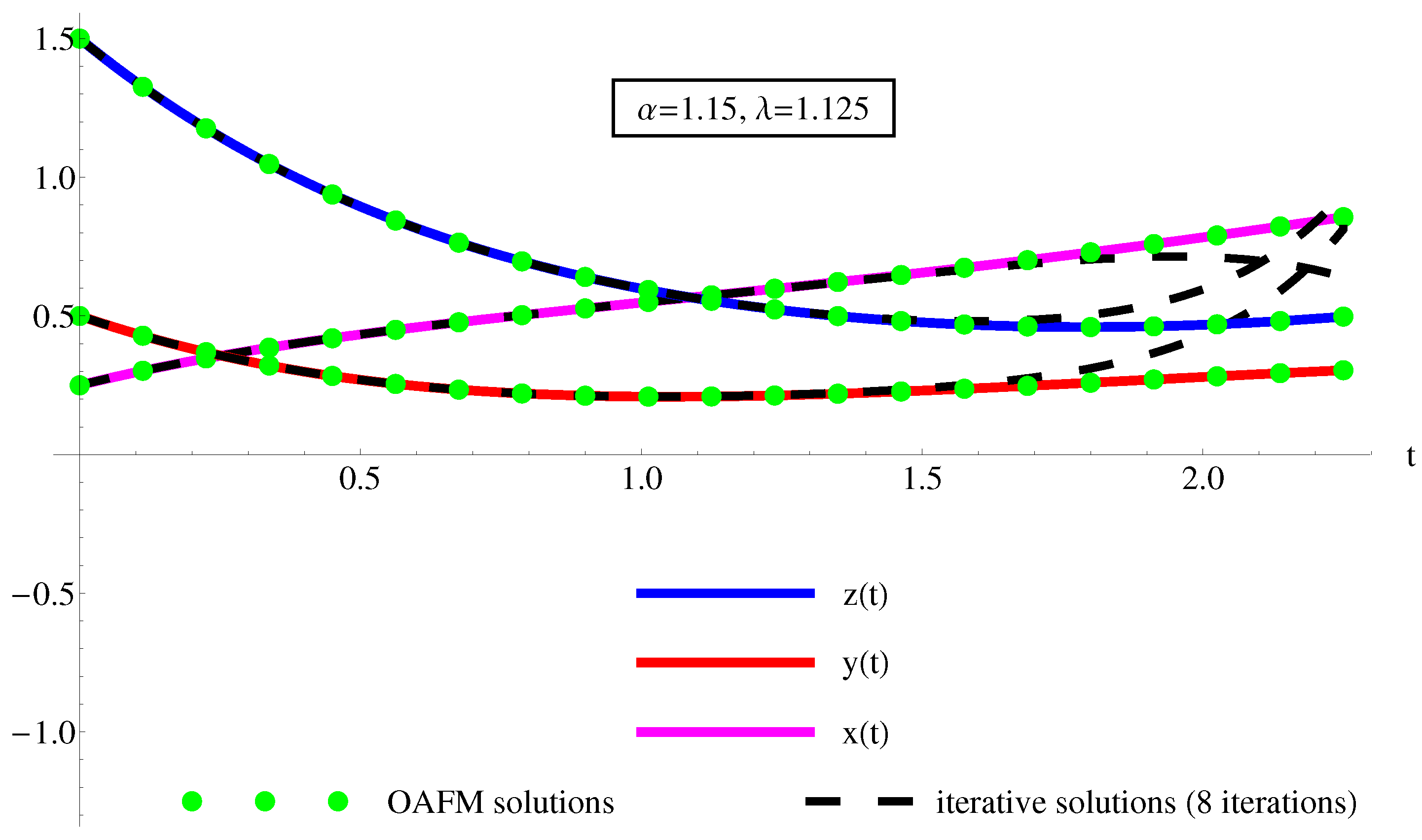
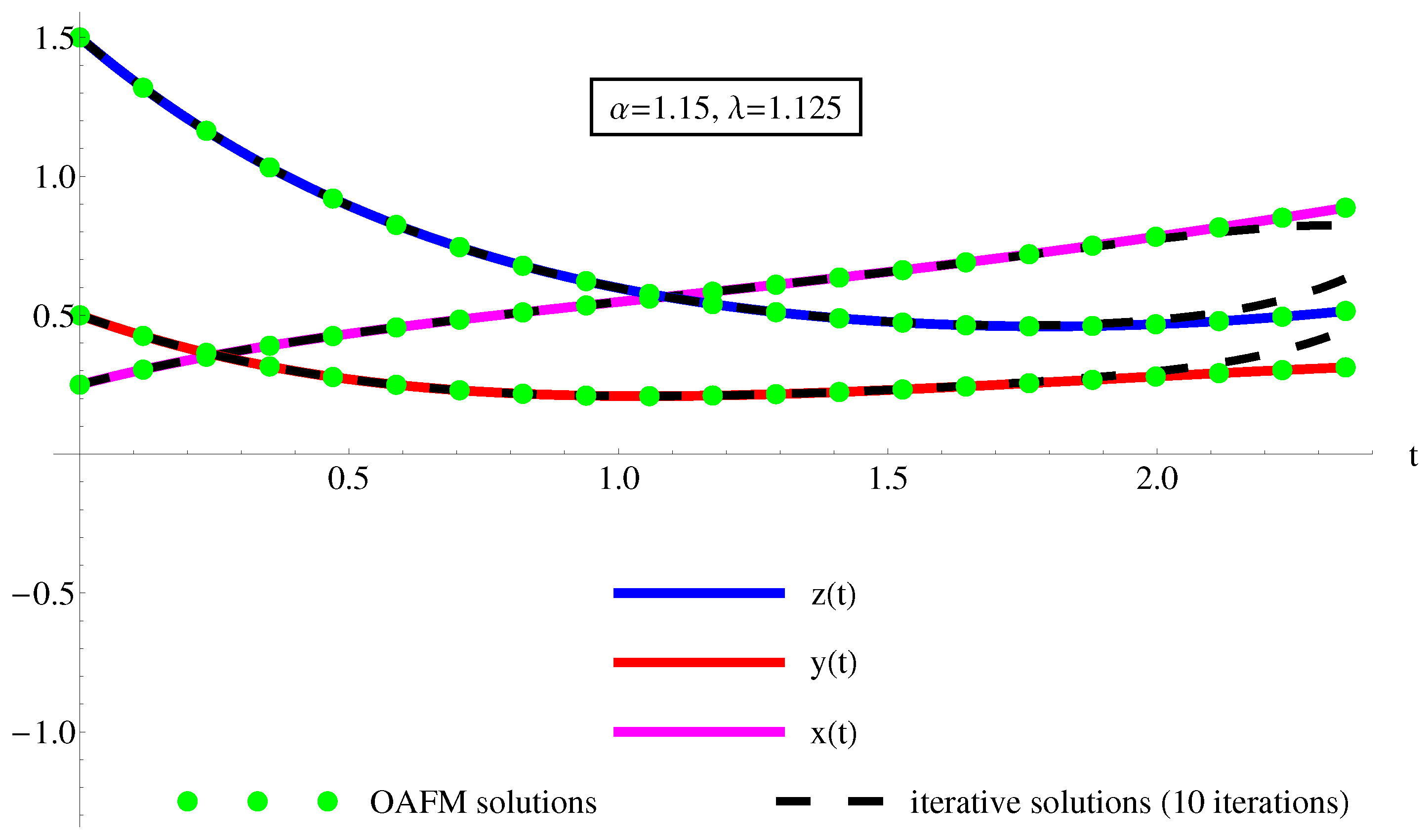
OAFM Technique Versus the Iterative Method

The choice of the OAFM method is justified by the comparison between the obtained results via the OAFM technique and the analytical solution obtained with the iterative method.

The iterative method developed by Daftardar-Gejji et al. [20] is proposed for solving nonlinear functional equations. This method is validated just for a special class of nonlinear functional equations with known exact solutions.

A simple integration of the system (1), yields

$$\begin{array}{c}{\displaystyle x\left(t\right)=x\left(0\right)+\underset{0}{\overset{t}{\int }}y\left(s\right)ds}\hfill \\ {\displaystyle y\left(t\right)=y\left(0\right)+\underset{0}{\overset{t}{\int }}\left(x\left(s\right)-\lambda y\left(s\right)-x\left(s\right)z\left(s\right)\right)ds}\hfill \\ {\displaystyle z\left(t\right)=z\left(0\right)+\underset{0}{\overset{t}{\int }}\left(x^2\left(s\right)-\alpha z\left(s\right)\right)ds}\hfill \end{array}.$$

(42)

The iterative scheme leads to

$$\begin{array}{c}{\displaystyle x_0\left(t\right)=x\left(0\right),x_1\left(t\right)=N_1(x_0,y_0,z_0)=\underset{0}{\overset{t}{\int }}y\left(0\right)ds,}\hfill \\ {\displaystyle y_0\left(t\right)=y\left(0\right),y_1\left(t\right)=N_2(x_0,y_0,z_0)=\underset{0}{\overset{t}{\int }}\left(x\left(0\right)+\lambda y\left(0\right)-x\left(0\right)z\left(0\right)\right)ds,}\hfill \\ {\displaystyle z_0\left(t\right)=z\left(0\right),z_1\left(t\right)=N_3(x_0,y_0,z_0)=\underset{0}{\overset{t}{\int }}\left(x^2\left(0\right)-\alpha z\left(0\right)\right)ds,}\hfill \\ \dots \hfill \\ x_m\left(t\right)=N_1\left({\displaystyle \sum _{i=0}^{m-1}{x}_i,\sum _{i=0}^{m-1}{y}_i,\sum _{i=0}^{m-1}{z}_i}\right)-N_1\left({\displaystyle \sum _{i=0}^{m-2}{x}_i,\sum _{i=0}^{m-2}{y}_i,\sum _{i=0}^{m-2}{z}_i}\right),\hfill \\ y_m\left(t\right)=N_2\left({\displaystyle \sum _{i=0}^{m-1}{x}_i,\sum _{i=0}^{m-1}{y}_i,\sum _{i=0}^{m-1}{z}_i}\right)-N_2\left({\displaystyle \sum _{i=0}^{m-2}{x}_i,\sum _{i=0}^{m-2}{y}_i,\sum _{i=0}^{m-2}{z}_i}\right),\hfill \\ z_m\left(t\right)=N_3\left({\displaystyle \sum _{i=0}^{m-1}{x}_i,\sum _{i=0}^{m-1}{y}_i,\sum _{i=0}^{m-1}{z}_i}\right)-N_3\left({\displaystyle \sum _{i=0}^{m-2}{x}_i,\sum _{i=0}^{m-2}{y}_i,\sum _{i=0}^{m-2}{z}_i}\right),\hfill \\ m\ge 2.\hfill \end{array}$$

(43)

The iterative solution generates the solution of Equations (1) as

$${\displaystyle x_{iter}\left(t\right)=\sum _{m=0}^{\infty }{x}_m\left(t\right),y_{iter}\left(t\right)=\sum _{m=0}^{\infty }{y}_m\left(t\right),z_{iter}\left(t\right)=\sum _{m=0}^{\infty }{z}_m\left(t\right),}$$

The iterative solutions $x_{iter}\left(t\right)$, after eight iterations using algorithm (43), for the initial data $x_{i0}=0.25$, $y_{i0}=0.5$, $z_{i0}=1.5$ and physical parameters $\alpha =1.15$, $\lambda =1.125$ (presented in

Table 4. The comparative values of the numerical solution, OAFM solution ${\overline{x}}_{OAFM}\left(t\right)$ using (A1) and the iterative solution $x_{iter}\left(t\right)$.

$\mathit{t}\left[\mathit{s}\right]$	${\mathit{x}}_{\mathit{numerical}}$	${\overline{\mathit{x}}}_{\mathit{OAFM}}$	${\mathit{x}}_{\mathit{iter}}$	${\mathit{x}}_{\mathit{iter}}$	${\mathit{x}}_{\mathit{iter}}$
			7 Iterations	8 Iterations	10 Iterations
0	0.25	0.2499999999	0.25	0.25	0.25
0.225	0.3468949150	0.3469078400	0.3468949335	0.3468949323	0.3505635497
0.45	0.4195412937	0.4195648239	0.4195417133	0.4195412626	0.4251520207
0.675	0.4771848531	0.4771926679	0.4771990261	0.4771831860	0.4841476700
0.9	0.5270086855	0.5270102734	0.5271821209	0.5269801371	0.5354682693
1.125	0.5741929869	0.5742109718	0.5754025051	0.5739364010	0.5846888548
1.35	0.6222786054	0.6223092588	0.6281794274	0.6207406723	0.6354400560
1.575	0.6735534955	0.6735731407	0.6961185567	0.6665968516	0.6895499112
1.8	0.7293586022	0.7293559010	0.8020100267	0.7038008705	0.7462081568
2.025	0.7902887499	0.7902778444	0.9973833252	0.7105500416	0.7986023305
2.25	0.8562977605	0.8562996826	1.3995527233	0.6398630067	0.8248310606

and

Table 5. The comparative values of the numerical solution, OAFM solution ${\overline{z}}_{OAFM}\left(t\right)$ using (A1) and the iterative solution $z_{iter}\left(t\right)$.

$\mathit{t}\left[\mathit{s}\right]$	${\mathit{z}}_{\mathit{numerical}}$	${\overline{\mathit{z}}}_{\mathit{OAFM}}$	${\mathit{z}}_{\mathit{iter}}$	${\mathit{z}}_{\mathit{iter}}$	${\mathit{z}}_{\mathit{iter}}$
			7 Iterations	8 Iterations	10 Iterations
0	1.5	1.5000000016	1.5	1.5	1.5
0.225	1.1763758373	1.1763763751	1.1763757896	1.1763757922	1.1641341787
0.45	0.9378639572	0.9378676478	0.9378631485	0.9378640152	0.9200664690
0.675	0.7643380562	0.7643437610	0.7643128002	0.7643410051	0.7452321079
0.9	0.6403948868	0.6403998115	0.6400984112	0.6404433398	0.6226403148
1.125	0.5547653149	0.5547710983	0.5527422169	0.5551927272	0.5401070051
1.35	0.4994768704	0.4994876016	0.4897131848	0.5020315716	0.4893266173
1.575	0.4690685160	0.4690836737	0.4320260737	0.4807569279	0.4654776866
1.8	0.4599450190	0.4599588459	0.3423976013	0.5041468859	0.4685787862
2.025	0.4698652175	0.4698731920	0.1453402602	0.6159658167	0.5098294719
2.25	0.4975217052	0.4975261008	−0.3062329520	0.9417127712	0.6322843547

), are built:

$$\begin{array}{c}{\displaystyle x_{iter}\left(t\right)=\sum _{m=0}^8{x}_m\left(t\right)=0.25+0.5t-0.34375t^2+0.1565104166t^3+0.0170556640t^4-}\hfill \\ 0.0584939697t^5+0.0378371174t^6-0.0127298036t^7+0.0004656224t^8+0.0021798576t^9-\hfill \\ 0.0014725273t^{10}+0.0003974510t^{11}+3.4181\times {10}^{-5}{t}^{12}-8.0516\times {10}^{-5}{t}^{13}+3.1132\times {10}^{-5}{t}^{14}-\hfill \\ 1.3113\times {10}^{-7}{t}^{15}-5.8882\times {10}^{-6}{t}^{16}+3.1387\times {10}^{-6}{t}^{17}-6.1138\times {10}^{-7}{t}^{18}-1.9112\times {10}^{-7}{t}^{19}+\hfill \\ 1.8377\times {10}^{-7}{t}^{20}-5.9641\times {10}^{-8}{t}^{21}+3.5149\times {10}^{-9}{t}^{22}+5.2124\times {10}^{-9}{t}^{23}-2.3107\times {10}^{-9}{t}^{24}+\hfill \\ 3.1591\times {10}^{-10}{t}^{25}+9.8039\times {10}^{-11}{t}^{26}-5.3142\times {10}^{-11}{t}^{27}+6.6353\times {10}^{-12}{t}^{28}+2.1138\times {10}^{-12}{t}^{29}-\hfill \\ 8.9186\times {10}^{-13}{t}^{30}+\mathcal{O}\left({10}^{-14}\right),\hfill \\ \\ {\displaystyle y_{iter}\left(t\right)=\sum _{m=0}^8{y}_m\left(t\right)=0.5-0.6875t+0.4695312499t^2+0.0682226562t^3-0.2924698486t^4+}\hfill \\ 0.2270227048t^5-0.0891086258t^6+0.0037249797t^7+0.0197403196t^8-0.0142001709t^9+\hfill \\ 0.0048737031t^{10}+1.9348\times {10}^{-4}{t}^{11}-0.0011328990t^{12}+5.9700\times {10}^{-4}{t}^{13}-8.3579\times {10}^{-5}{t}^{14}-\hfill \\ 8.9044\times {10}^{-5}{t}^{15}+7.2833\times {10}^{-5}{t}^{16}-2.4277\times {10}^{-5}{t}^{17}-9.4457\times {10}^{-7}{t}^{18}+5.5099\times {10}^{-6}{t}^{19}-\hfill \\ 3.0123\times {10}^{-6}{t}^{20}+6.9622\times {10}^{-7}{t}^{21}+1.3734\times {10}^{-7}{t}^{22}-1.8410\times {10}^{-7}{t}^{23}+7.0785\times {10}^{-8}{t}^{24}-\hfill \\ 6.6210\times {10}^{-9}{t}^{25}-7.1580\times {10}^{-9}{t}^{26}+4.1566\times {10}^{-9}{t}^{27}-8.3207\times {10}^{-10}{t}^{28}-2.0864\times {10}^{-10}{t}^{29}+\hfill \\ 1.9970\times {10}^{-10}{t}^{30}-5.5930\times {10}^{-11}{t}^{31}-2.4605\times {10}^{-12}{t}^{32}+7.8517\times {10}^{-12}{t}^{33}-2.7870\times {10}^{-12}{t}^{34}+\hfill \\ 1.7604\times {10}^{-13}{t}^{35}+2.3476\times {10}^{-13}{t}^{36}-1.0123\times {10}^{-13}{t}^{37}+1.1642\times {10}^{-14}{t}^{38}+\mathcal{O}\left({10}^{-15}\right),\hfill \\ {\displaystyle z_{iter}\left(t\right)=\sum _{m=0}^8{z}_m\left(t\right)=1.5-1.6625t+1.0809375t^2-0.3883177083t^3+0.0452676432t^4+}\hfill \\ 0.0462289042t^5-0.0288259120t^6+9.0630\times {10}^{-4}{t}^7+0.0094979185t^8-0.0074539538t^9+\hfill \\ 0.0029479799t^{10}-7.7601\times {10}^{-5}{t}^{11}-6.3838\times {10}^{-4}{t}^{12}+4.3420\times {10}^{-4}{t}^{13}-1.3675\times {10}^{-4}{t}^{14}-\hfill \\ 2.4645\times {10}^{-6}{t}^{15}+2.6082\times {10}^{-5}{t}^{16}-1.3709\times {10}^{-5}{t}^{17}+2.8875\times {10}^{-6}{t}^{18}+6.9597\times {10}^{-7}{t}^{19}-\hfill \\ 7.5299\times {10}^{-7}{t}^{20}+2.3692\times {10}^{-7}{t}^{21}+6.5685\times {10}^{-9}{t}^{22}-3.7993\times {10}^{-8}{t}^{23}+1.5694\times {10}^{-8}{t}^{24}-\hfill \\ 1.2902\times {10}^{-9}{t}^{25}-1.6918\times {10}^{-9}{t}^{26}+9.1570\times {10}^{-10}{t}^{27}-1.6639\times {10}^{-10}{t}^{28}-4.5309\times {10}^{-11}{t}^{29}+\hfill \\ 3.6967\times {10}^{-11}{t}^{30}-8.5148\times {10}^{-12}{t}^{31}-1.0466\times {10}^{-12}{t}^{32}+1.2857\times {10}^{-12}{t}^{33}-3.2713\times {10}^{-13}{t}^{34}-\hfill \\ 2.2946\times {10}^{-14}{t}^{35}+4.0185\times {10}^{-14}{t}^{36}-1.0989\times {10}^{-14}{t}^{37}+\mathcal{O}\left({10}^{-16}\right).\hfill \end{array}$$

(44)

The performance of the OAFM method is comparative to the iterative method (using 7–10 iterations) results from Table 4 and Table 5 and Figure 6, Figure 7 and Figure 8. By analyzing these results, it is clear that by increasing the number of iterations, the performance of the iterative method becomes competitive to the OAFM method.

4. Conclusions

This article demonstrated damped oscillations behaviors for solutions of the Shimizu–Morioka dynamical system using the OAFM approach. The dynamics of the system is influenced by values of the physical parameters $\alpha$ and $\lambda$.

A good agreement between the OAFM results and the corresponding numerical ones are highlighted in this work. The comparative analysis reflects the accuracy of the method; the obtained solutions are approaching the exact solution.

OAFM solutions are built for the chosen values for the physical parameters $\alpha$, $\lambda$ such that the asymptotic stability of equilibrium point $E_{+}$ is satisfied, e.g., $\alpha +\lambda >0$, $\alpha >0$, $(\alpha +\lambda )\lambda >2$. In this work are presented in detail two cases corresponding to (i) $\alpha ,\lambda >1$, arbitrarily chosen, and (ii) $\alpha ,\lambda \in (0,\sqrt{2})$, where $(2\sqrt{4+{\lambda }^2}+\alpha )/\left(2\alpha \right)$ is not an integer number.

The advantages of the OAFM method comparative to other analytical methods are synthesized by the following:

• The arbitrary choice of the linear operator L and auxiliary functions $A_j$ allows writing the OAFM solution in effective form;
• The convergence control is ensured by the residual functions being smaller than 1);
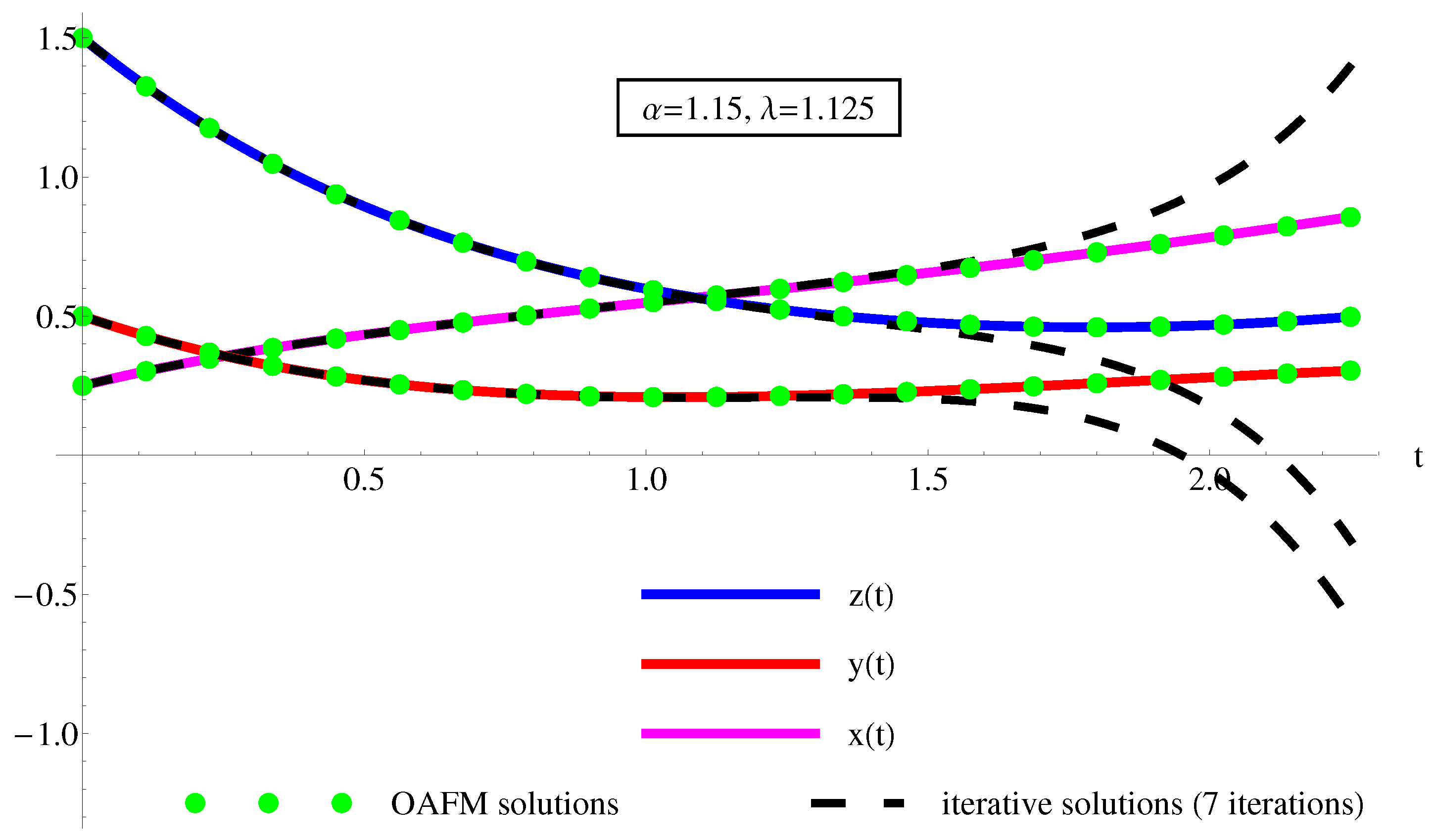
• The comparison between the OAFM solutions with the iterative corresponding using 7, 8, 10 iterations highlights the efficiency of the OAFM method by arbitrarily choosing the auxiliary functions and optimally finding the unknown parameters.

References

1. Huang, K.; Shi, S.; Li, W. Integrability analysis of the Shimizu-Morioka system. Commun. Nonlinear Sci. Numer. Simulat. 2020, 84, 105101. [Google Scholar] [CrossRef]
2. Chen, Z.; Wen, G.; Zhou, H.; Chen, J. A new M × N-grid double-scroll chaotic attractors from Rucklidge chaotic system. Optik 2017, 136, 27–35. [Google Scholar] [CrossRef]
3. Lorenz, E.N. Deterministic nonperiodic flow. J. Atmos. Sci. 1963, 20, 130–141. [Google Scholar] [CrossRef]
4. Shimizu, T.; Morioka, N. On the bifurcation of a symmetric limit cycle to an asymmetric one in a simple model. Phys. Lett. A 1980, 76, 201–204. [Google Scholar] [CrossRef]
5. Rucklidge, A.M. Chaos in models of double convection. J. Fluid Mech. 1992, 237, 209–229. [Google Scholar] [CrossRef]
6. Wei, Z.; Zhang, X. Chaos in the Shimizu-Morioka Model with Fractional Order. Front. Phys. 2021, 9, 636173. [Google Scholar] [CrossRef]
7. Pyragas, V.; Pyragas, K. Modification of delayed feedback control using ergodicity of chaotic systems. Lith. J. Physics 2010, 50, 305–316. [Google Scholar] [CrossRef]
8. El-Dessoky, M.M.; Yassen, M.T.; Aly, E.S. Bifurcation analysis and chaos control in Shimizu-Morioka chaotic system with delayed feedback. Appl. Math. Comput. 2014, 243, 283–297. [Google Scholar] [CrossRef]
9. Hajiloo, R.; Salarieh, H.; Alasty, A. Chaos control in delayed phase space constructed by the Takens embedding theory. Commun. Nonlinear Sci. Numer. Simulat. 2018, 54, 453–465. [Google Scholar] [CrossRef]
10. Dong, C.; Lian, J.; Qi, J.; Hantao, L. Symbolic Encoding of Periodic Orbits and Chaos in the Rucklidge System. Complexity 2021, 2021, 4465151. [Google Scholar] [CrossRef]
11. Zhang, X. Stability and bifurcation analysis for a delayed Shimizu-Morioka model. Miskolc Math. Notes 2019, 20, 585–598. [Google Scholar] [CrossRef]
12. Llibre, J.; Pessoa, C. The Hopf bifurcation in the Shimizu-Morioka system. Nonlinear Dyn. 2015, 79, 2197–2205. [Google Scholar] [CrossRef]
13. Lazureanu, C.; Cho, J. On the dynamics of a deformed version of the Shimizu-Morioka system. Sci. Bull. Politeh. Timis. Trans. Math. Phys. 2021, 66, 3–28. [Google Scholar]
14. Tarammim, A.; Akter, M.T. Shimizu-Morioka’s chaos synchronization: An efficacy analysis of active control and backstepping methods. Front. Appl. Math. Stat. 2023, 9, 1100147. [Google Scholar] [CrossRef]
15. Marinca, V.; Herisanu, N. Approximate analytical solutions to Jerk equation. In Springer Proceedings in Mathematics & Statistics: Proceedings of the Dynamical Systems: Theoretical and Experimental Analysis, Lodz, Poland, 7–10 December 2015; Springer: Cham, Switzerland, 2016; Volume 182, pp. 169–176. [Google Scholar]
16. Marinca, V.; Ene, R.-D.; Marinca, V.B. Optimal Auxiliary Functions Method for viscous flow due to a stretching surface with partial slip. Open Eng. 2018, 8, 261–274. [Google Scholar] [CrossRef]
17. Ene, R.-D.; Pop, N.; Lapadat, M. Approximate Closed-Form Solutions for the Rabinovich System via the Optimal Auxiliary Functions Method. Symmetry 2022, 14, 2185. [Google Scholar] [CrossRef]
18. Ene, R.-D.; Pop, N.; Lapadat, M.; Dungan, L. Approximate closed-form solutions for the Maxwell-Bloch equations via the Optimal Homotopy Asymptotic Method. Mathematics 2022, 10, 4118. [Google Scholar] [CrossRef]
19. Ene, R.-D.; Pop, N.; Badarau, R. Exact Parametric and Semi-Analytical Solutions for the Rucklidge-Type Dynamical System. Mathematics 2025, 13, 2052. [Google Scholar] [CrossRef]
20. Daftardar-Gejji, V.; Jafari, H. An iterative method for solving nonlinear functional equations. J. Math. Anal. Appl. 2006, 316, 753–763. [Google Scholar] [CrossRef]
Figure 1. States of the system (1) ( x ¯ O A F M , y ¯ O A F M , z ¯ O A F M ) using Equations (30), (31) and (A1) for x i 0 = 0.25 , y i 0 = 0.5 , z i 0 = 1.5 , physical parameters α = 1.15 , λ = 1.125 (c1dotted curves) in comparison with the numerical integration results (solid curves: red for x ( t ) , green curve for y ( t ) , blue for z ( t ) ).
Axioms 14 00580 g001
Figure 2. States of the system (1) ( x ¯ O A F M , y ¯ O A F M , z ¯ O A F M ) using Equations (40), (31) and (A2) for x i 0 = 0.25 , y i 0 = 0.5 , z i 0 = 1.5 , physical parameters α = 0.15 , λ = 0.125 (dotted curves ) by comparison with numerical integration results (solid curves: red for x ( t ) , green curve for y ( t ) , blue for z ( t ) ).
Axioms 14 00580 g002
Figure 3. States of the system (1) ( x ¯ O A F M , y ¯ O A F M ) using Equations (40), (31) and (A3) for x i 0 = 0.25 , y i 0 = 0.5 , z i 0 = 1.5 , physical parameters α = 0.41 , λ = 0.84 (dotted curves ) by comparison with numerical integration results (solid curves: red for x ( t ) , green curve for y ( t ) , blue for z ( t ) ).
Axioms 14 00580 g003
Figure 4. The variation of the residual function given by (41) for y ¯ O A F M for x i 0 = 0.25 , y i 0 = 0.5 , z i 0 = 1.5 , physical constants α = 1.15 , λ = 1.125 .
Axioms 14 00580 g004
Figure 5. Rucklidge (solid curves) versus Shimizu–Morioka (dotted curves) OAFM solutions ( x ¯ O A F M , y ¯ O A F M , z ¯ O A F M ) for: x i 0 = 0.25 , y i 0 = 0.5 , z i 0 = 1.5 , physical parameters: α = 1.150 , λ = 1.125 (solid curves: red for x ( t ) , green curve for y ( t ) , blue for z ( t ) ).
Axioms 14 00580 g005
Figure 6. The accuracy of the semi-analytical solutions x ¯ O A F M ( t ) , y ¯ O A F M ( t ) , z ¯ O A F M ( t ) of Equation (1) using Equation (A1) (dotted green curves), by comparison with the iterative solutions (7 iterations) x i t e r ( t ) , y i t e r ( t ) , z i t e r ( t ) using Equation (44) (dashing black curves) and the corresponding numerical ones (solid color curves: magenta for x ( t ) , red for y ( t ) , and blue for z ( t ) ), respectively.
Axioms 14 00580 g006
Figure 7. The accuracy of the semi-analytical solutions x ¯ O A F M ( t ) , y ¯ O A F M ( t ) , z ¯ O A F M ( t ) of Equation (1) using Equation (A1) (dotted green curves), by comparison with the iterative solutions (8 iterations) x i t e r ( t ) , y i t e r ( t ) , z i t e r ( t ) using Equation (44) (dashing black curves) and the corresponding numerical ones (solid color curves: magenta for x ( t ) , red for y ( t ) , and blue for z ( t ) ), respectively.
Axioms 14 00580 g007
Figure 8. The accuracy of the semi-analytical solutions x ¯ O A F M ( t ) , y ¯ O A F M ( t ) , z ¯ O A F M ( t ) of Equation (1) using Equation (A1) (dotted green curves), by comparison with the iterative solutions (10 iterations) x i t e r ( t ) , y i t e r ( t ) , z i t e r ( t ) using Equation (44) (dashing black curves) and the corresponding numerical ones (solid color curves: magenta for x ( t ) , red for y ( t ) , and blue for z ( t ) ), respectively.
Axioms 14 00580 g008