On Joint Progressively Censored Gumbel Type-II Distributions: (Non-) Bayesian Estimation with an Application to Physical Data

Abstract

This paper presents a comprehensive statistical analysis of the Gumbel Type-II distribution based on joint progressive Type-II censoring. It derives the maximum likelihood estimators for the distribution parameters and constructs their asymptotic confidence intervals. It investigates Bayesian estimation using non-informative and informative priors under the squared error loss function and the LINEX loss function, applying Markov Chain Monte Carlo methods. A detailed simulation study evaluates the estimators’ performance in terms of average estimates, mean squared errors, and average confidence interval lengths. Results show that Bayesian estimators can outperform maximum likelihood estimators, especially with informative priors. A real data example demonstrates the practical use of the proposed methods. The analysis confirms that the Gumbel Type-II distribution with joint progressive censoring provides a flexible and effective model for lifetime data, enabling more accurate reliability assessment and risk analysis in engineering and survival studies.

1. Introduction

The Gumbel Type-II (G-II) distribution, introduced by the German mathematician Emil Gumbel [1], serves as an essential model for extreme value analysis, such as floods, earthquakes, and other natural disasters. It is also used in a number of disciplines, such as rainfall studies, hydrology, and life expectancy tables. In comparative longevity tests, Gumbel emphasized its remarkable ability to replicate the anticipated lifespan of products. Moreover, this distribution plays a crucial role in forecasting the likelihood of climatic events and natural catastrophes.

Over the years, numerous researchers have advanced statistical inference techniques for the G-II distribution, such as Mousa et al. [2], Malinowska and Szynal [3], Miladinovic and Tsokos [4], Nadarajah and Kotz [5], Feroze and Aslam [6], Abbas et al. [7], Feroze and Aslam [8], Reyad and Ahmed [9], Sindhu et al. [10], Abbas et al. [11], and Qiu and Gui [12]. For $\theta >0$ and $\sigma >0$, the cumulative distribution function (CDF) of the G-II distribution is given as follows:

$$F\left(x\right)=e^{-\theta x^{-\sigma }},x>0,\theta >0,\sigma >0,$$

(1)

Moreover, the corresponding probability density function (PDF) is provided as follows:

$$f\left(x\right)=\theta \sigma x^{-(\sigma +1)}{e}^{-\theta x^{-\sigma }},x>0,\theta >0,\sigma >0.$$

(2)

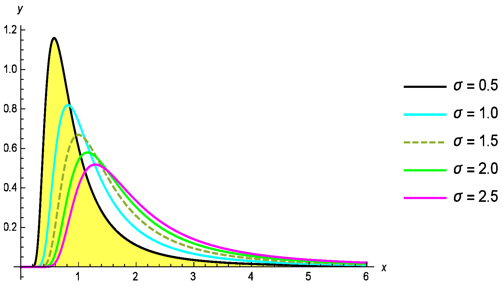
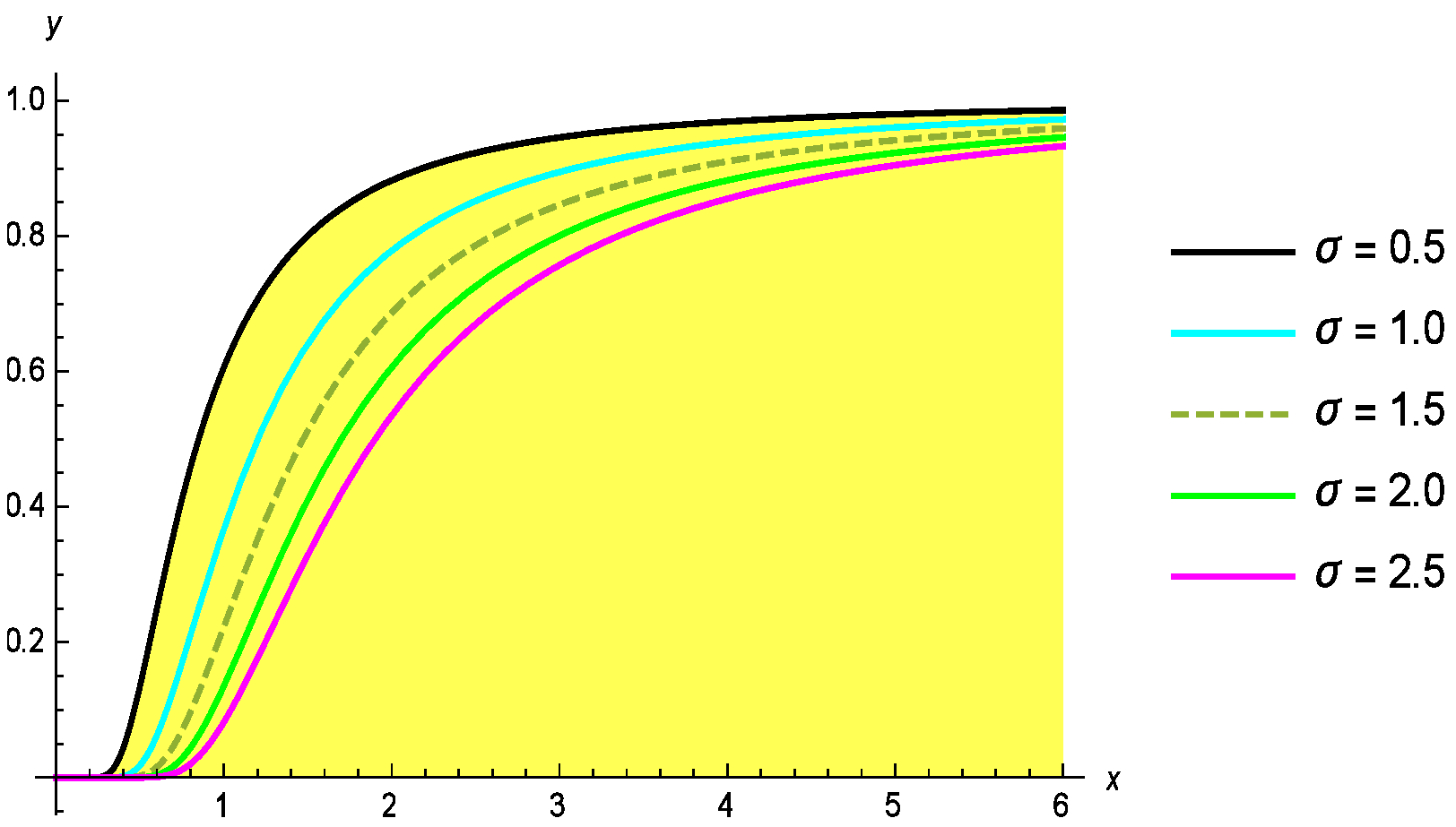
Here, the shape and scale parameters are denoted by $\sigma$ and $\theta$, respectively. The probability density function (PDF) and cumulative distribution function (CDF) of the G-II distribution for different values of the parameters $\theta$ and $\sigma$ are shown in Figure 1 and Figure 2.

Censored data is prevalent in various fields, including science, public health, and medicine, making it essential to implement an appropriate censoring scheme. One of the most widely recognized methods is progressive Type-II censoring. In this approach, the number of observed failures, denoted as m (where $m\le n$), is predetermined along with a censoring scheme $R=(R_1,\dots ,R_m)$. At each i-th failure, a specified number of remaining units are randomly removed from the experiment. This method offers the dual advantage of reducing both cost and time by allowing the removal of surviving units during the trial. Due to these benefits, progressive Type-II censoring has gained significant attention and has been extensively studied in the literature [13,14,15,16,17].

Implementing censoring strategies on a single group can present several challenges. Although progressive Type-II censoring allows for the removal of certain data points, obtaining a sufficient number of observations remains costly. Moreover, studying group reliability and interactions, which cannot be adequately captured through experiments involving only one group, is often a key objective. To address these limitations, Rasouli and Balakrishnan [18] proposed the Joint Progressive Censoring Scheme (Joint PCS). This approach enables the occurrence of failures in two groups simultaneously, effectively halving the time required to collect the same volume of data. Additionally, the Joint PCS facilitates the comparison of failure times between the two groups under identical experimental conditions, enhancing the robustness and applicability of the results.

Initially, groups A and B contain m and n units, respectively. The Joint PCS method originates from a life-testing experiment involving these two groups. The expected number of failures, denoted as $ϵ$, is predetermined. The failure points are represented by ${\phi }_1,\dots ,{\phi }_{ϵ}$. At each failure time, $s_i$ surviving units from group A and $t_i$ units from group B are randomly removed. Thus, at the i-th failure, a total of $R_i=s_i+t_i$ units are eliminated. Additionally, a second set of random variables, ${\nu }_1,\dots ,{\nu }_{ϵ}$, is introduced, where each variable takes a value of either 1 or 0. These values indicate the source of the failure as follows:

$${\nu }_i=\left\{\begin{array}{cc}1\hfill & \mathrm{if}{\phi }_i\mathrm{is}\mathrm{from}\mathrm{group}A,\hfill \\ 0\hfill & \mathrm{if}{\phi }_i\mathrm{is}\mathrm{from}\mathrm{group}B.\hfill \end{array}\right.$$

The censored sample is represented as $(({\phi }_1,{\nu }_1,s_1),\dots ,({\phi }_{ϵ},{\nu }_{ϵ},s_{ϵ}))$. Here, ${ϵ}_1={\sum }_{i=1}^{ϵ}{\nu }_i$ represents the total number of failures from group A. Similarly, ${ϵ}_2={\sum }_{i=1}^{ϵ}(1-{\nu }_i)=ϵ-{ϵ}_1$ indicates the number of failures from group B.

The Joint PCS has generated substantial interest among researchers. Several authors have examined Joint PCS and its related inference techniques, contributing to a rich body of literature. Across various applications, numerous scholars have explored a wide range of methodologies and heterogeneous lifetime models. For further reading, the works of [19,20,21,22,23,24,25,26,27,28,29,30,31] are recommended.

This manuscript makes significant contributions to the estimation of unknown parameters for the G-II distribution under a joint PCS, which is widely used in reliability analysis and lifetime data modeling. It employs both classical and Bayesian inference methods, utilizing maximum likelihood estimation (MLE) for point and interval estimation in the frequentist framework and Bayesian estimation (BE) via Markov Chain Monte Carlo (MCMC) methods, specifically the Metropolis–Hastings (M–H) algorithm, to handle complex posterior computations. Asymptotic confidence intervals (ACIs) and highest posterior density (HPD) credible intervals (CRIs) are derived to provide a comprehensive uncertainty assessment. The study explores the impact of different loss functions on Bayesian estimators. Through extensive Monte Carlo simulations, it evaluates the efficiency of the proposed estimation techniques by analyzing point estimates, interval estimates, and mean squared errors (MSE), demonstrating that Bayesian methods provide more precise and efficient estimates than MLE, particularly when informative priors are available. Additionally, the practical effectiveness of the proposed methodologies is validated through a real dataset, reinforcing their applicability in reliability analysis. Despite these contributions, the study encounters challenges in handling complex likelihood functions analytically, necessitating computational methods for parameter estimation. The selection of prior distributions in Bayesian inference and the computational burden of MCMC methods also pose difficulties. Moreover, while joint progressive censoring enhances efficiency in data collection, achieving a balance between cost, time, and sufficient observations remains a challenge. Overall, this study advances statistical inference for extreme value distributions by enhancing parameter estimation under joint PCS and offering a robust methodological framework applicable across various scientific and engineering disciplines.

The main goal of this study is to develop and compare estimation methods for the G-II distribution under a joint PCS by employing both classical MLE and Bayesian inference with different loss functions. The study introduces novelty by being the first to provide comprehensive parameter estimation for this distribution using joint progressive censoring, incorporating ACIs and highest posterior density CRIs, and applying squared error and LINEX loss functions in the Bayesian framework. It also uses the M–H MCMC algorithm to handle complex posterior computations and validates the proposed methods with real-world failure data, demonstrating their effectiveness in lifetime and reliability analysis.

The remainder of the paper is structured as follows. Section 2 develops the model, derives point estimates using the MLE method, and obtains ACIs. Section 3 presents BEs of the parameters under different loss functions, along with the proposed MCMC algorithm. Section 4 includes a simulation study to compare the proposed methods. Section 5 demonstrates the application of the inference procedures using a real-life dataset. Finally, Section 6 provides concluding remarks.

2. Classical Inference

Classical inference, also known as frequentist inference, is a fundamental approach in statistical analysis that relies on probability models to draw conclusions about unknown parameters. It is based on the concept of repeated sampling, where estimators are evaluated in terms of their long-run properties, such as unbiasedness, consistency, and efficiency. Methods like MLE and the Method of Moments are commonly used to estimate parameters, while hypothesis testing and confidence intervals provide a framework for decision-making. Unlike Bayesian inference, classical inference does not incorporate prior information and relies solely on observed data. This approach is widely used in scientific research due to its well-established theoretical foundations and objective interpretation of results.

2.1. Maximum Likelihood Estimation

If $X_1,\dots ,X_m$ represent observations from group A, then $Y_1,\dots ,Y_n$ correspond to observations from group B. The observed data, denoted as $({\phi }_1,{\nu }_1,s_1,t_1),\dots ,({\phi }_{ϵ},{\nu }_{ϵ},s_{ϵ},t_{ϵ})$, follow a specified joint PCS $(R_1,\dots ,R_{ϵ})$. Throughout the subsequent sections, the term “data” refers to the censored dataset $({\phi }_1,{\nu }_1,s_1,t_1),\dots ,({\phi }_{ϵ},{\nu }_{ϵ},s_{ϵ},t_{ϵ})$. The likelihood function is formulated as follows:

$$L({\sigma }_1,{\sigma }_2,{\theta }_1,{\theta }_2|data)=\prod _{i=1}^{ϵ}\left[{\left[f\left({\phi }_i\right)\right]}^{{\nu }_i}{\left[w\left({\phi }_i\right)\right]}^{1-{\nu }_i}\right]{\left[\overline{F}\left({\phi }_i\right)\right]}^{s_i}{\left[\overline{W}\left({\phi }_i\right)\right]}^{t_i},$$

(3)

${\phi }_1\le {\phi }_2\le \dots \le {\phi }_{ϵ}$, $\overline{F}=1-F$, $\overline{W}=1-W$, and ${\sum }_{i=1}^{ϵ}{s}_i+{\sum }_{i=1}^{ϵ}{t}_i={\sum }_{i=1}^{ϵ}{R}_i$.

By incorporating the CDF and PDF derived from Equations (1) and (2), respectively, into the likelihood equation in (3), the following result is obtained.

$$\begin{array}{cc}\hfill L({\sigma }_1,{\sigma }_1,{\theta }_1,{\theta }_2|data)=& {\sigma }_1^{{ϵ}_1}{\theta }_1^{{ϵ}_1}{\sigma }_2^{{ϵ}_2}{\theta }_2^{{ϵ}_2}{e}^{-({\sigma }_1+1){\sum }_{i=1}^{ϵ}{\nu }_{i}ln{\phi }_i}{e}^{-({\sigma }_2+1){\sum }_{i=1}^{ϵ}(1-{\nu }_i)ln{\phi }_i}{e}^{-{\theta }_1{\sum }_{i=1}^{ϵ}{\nu }_i{\phi }_i^{-{\sigma }_1}}\hfill \\ & \times e^{-{\theta }_2{\sum }_{i=1}^{ϵ}(1-{\nu }_i){\phi }_i^{-{\sigma }_2}}{e}^{{\sum }_{i=1}^{ϵ}{s}_{i}ln\left[1-e^{-{\theta }_1{\phi }_i^{-{\sigma }_1}}\right]}{e}^{{\sum }_{i=1}^{ϵ}{t}_{i}ln\left[1-e^{-{\theta }_2{\phi }_i^{-{\sigma }_2}}\right]}.\hfill \end{array}$$

(4)

The log-likelihood function, $\ell ({\sigma }_1,{\sigma }_2,{\theta }_1,{\theta }_2\mid \mathrm{data})$, is defined as the natural logarithm of the likelihood function $L({\sigma }_1,{\sigma }_2,{\theta }_1,{\theta }_2\mid \mathrm{data})$ and is expressed as follows:

$$\begin{array}{cc}\hfill \ell ({\sigma }_1,{\sigma }_2,{\theta }_1,{\theta }_2|data)=& {ϵ}_{1}ln{\sigma }_1+{ϵ}_{1}ln{\theta }_1+{ϵ}_{2}ln{\sigma }_2+{ϵ}_{2}ln{\theta }_2-({\sigma }_1+1)\sum _{i=1}^{ϵ}{\nu }_{i}ln{\phi }_i\hfill \\ & -({\sigma }_2+1)\sum _{i=1}^{ϵ}(1-{\nu }_i)ln{\phi }_i-{\theta }_1\sum _{i=1}^{ϵ}{\nu }_i{\phi }_i^{-{\sigma }_1}-{\theta }_2\sum _{i=1}^{ϵ}(1-{\nu }_i){\phi }_i^{-{\sigma }_2}\hfill \\ & +\sum _{i=1}^{ϵ}{s}_{i}ln\left[1-e^{-{\theta }_1{\phi }_i^{-{\sigma }_1}}\right]+\sum _{i=1}^{ϵ}{t}_{i}ln\left[1-e^{-{\theta }_2{\phi }_i^{-{\sigma }_2}}\right]\hfill \end{array}$$

(5)

By taking the partial derivatives of Equation (5), we derive the normal equations for the unknown parameters ${\sigma }_1$, ${\sigma }_2$, ${\theta }_1$, and ${\theta }_2$. The resulting expressions are then set to zero. Solving these equations yields the estimators $\widehat{{\sigma }_1}$, $\widehat{{\sigma }_2}$, $\widehat{{\theta }_1}$, and $\widehat{{\theta }_2}$ for the respective parameters.

$${\displaystyle \frac{{ϵ}_1}{{\sigma }_1}}-\sum _{i=1}^{ϵ}{\nu }_{i}ln{\phi }_i+{\theta }_1\sum _{i=1}^{ϵ}\nu {\phi }_i^{-{\sigma }_1}ln{\phi }_i-\sum _{i=1}^{ϵ}{\displaystyle \frac{s_i{e}^{-{\theta }_1{\phi }_i^{-{\sigma }_1}}{\theta }_1{\phi }_i^{-{\sigma }_1}ln{\phi }_i}{1-e^{-{\theta }_1{\phi }_i^{-{\sigma }_1}}}}=0,$$

(6)

$${\displaystyle \frac{{ϵ}_2}{{\sigma }_2}}-\sum _{i=1}^{ϵ}(1-{\nu }_i)ln{\phi }_i+{\theta }_2\sum _{i=1}^{ϵ}(1-\nu ){\phi }_i^{-{\sigma }_2}ln{\phi }_i-\sum _{i=1}^{ϵ}{\displaystyle \frac{t_i{e}^{-{\theta }_2{\phi }_i^{-{\sigma }_2}}{\theta }_2{\phi }_i^{-{\sigma }_2}ln{\phi }_i}{1-e^{-{\theta }_2{\phi }_i^{-{\sigma }_2}}}}=0,$$

(7)

$${\displaystyle \frac{-{ϵ}_1}{{\theta }_1}}-\sum _{i=1}^{ϵ}{\nu }_i{\phi }_i^{-{\sigma }_1}+\sum _{i=1}^{ϵ}{\displaystyle \frac{s_i{e}^{-{\theta }_1{\phi }_i^{-{\sigma }_1}}{\phi }_i^{-{\sigma }_1}}{1-e^{-{\theta }_1{\phi }_i^{-{\sigma }_1}}}}=0,$$

(8)

$${\displaystyle \frac{-{ϵ}_2}{{\theta }_2}}-\sum _{i=1}^{ϵ}(1-{\nu }_i){\phi }_i^{-{\sigma }_2}+\sum _{i=1}^{ϵ}{\displaystyle \frac{t_i{e}^{-{\theta }_2{\phi }_i^{-{\sigma }_2}}{\phi }_i^{-{\sigma }_2}}{1-e^{-{\theta }_2{\phi }_i^{-{\sigma }_2}}}}=0.$$

(9)

Since the resulting system of nonlinear equations lacks closed-form solutions, the first derivatives of the log-likelihood function with respect to each parameter, as given in Equations (6)–(9), cannot be determined analytically. Consequently, the MLEs must be computed using iterative numerical approximation methods. One effective approach for obtaining these estimates is the Newton–Raphson iteration method.

Existence and Uniqueness of MLEs

This part analyzes the existence and uniqueness of the MLEs for the unknown model parameters. Define

• $G_{{\sigma }_1}\left({\sigma }_1\right)={\displaystyle \frac{\partial \ell }{\partial {\sigma }_1}}$,
• $G_{{\sigma }_2}\left({\sigma }_2\right)={\displaystyle \frac{\partial \ell }{\partial {\sigma }_2}}$,
• $G_{{\theta }_1}\left({\theta }_1\right)={\displaystyle \frac{\partial \ell }{\partial {\theta }_1}}$,
• $G_{{\theta }_2}\left({\theta }_2\right)={\displaystyle \frac{\partial \ell }{\partial {\theta }_2}}$.

From Equation (6), if ${\sigma }_1>0$ is fixed, we find

$$\underset{{\sigma }_1\to 0}{lim}{G}_{{\sigma }_1}\left({\sigma }_1\right)\to +\infty ,$$

and

$$\underset{{\sigma }_1\to \infty }{lim}{G}_{{\sigma }_1}\left({\sigma }_1\right)\to -\sum _{i=1}^{ϵ}{\nu }_{i}ln{\phi }_i+{\theta }_1\sum _{i=1}^{ϵ}\nu {\phi }_i^{-{\sigma }_1}ln{\phi }_i-\sum _{i=1}^{ϵ}{\displaystyle \frac{s_i{e}^{-{\theta }_1{\phi }_i^{-{\sigma }_1}}{\theta }_1{\phi }_i^{-{\sigma }_1}ln{\phi }_i}{1-e^{-{\theta }_1{\phi }_i^{-{\sigma }_1}}}}=0.$$

(10)

Similarly, using Equation (7), we obtain

$$\underset{{\sigma }_2\to 0}{lim}{G}_{{\sigma }_2}\left({\sigma }_2\right)\to +\infty ,$$

and

$$\underset{{\sigma }_2\to \infty }{lim}{G}_{{\sigma }_2}\left({\sigma }_2\right)\to -\sum _{i=1}^{ϵ}(1-{\nu }_i)ln{\phi }_i+{\theta }_2\sum _{i=1}^{ϵ}(1-\nu ){\phi }_i^{-{\sigma }_2}ln{\phi }_i-\sum _{i=1}^{ϵ}{\displaystyle \frac{t_i{e}^{-{\theta }_2{\phi }_i^{-{\sigma }_2}}{\theta }_2{\phi }_i^{-{\sigma }_2}ln{\phi }_i}{1-e^{-{\theta }_2{\phi }_i^{-{\sigma }_2}}}}=0.$$

(11)

From Equation (8), if ${\theta }_1>0$ is fixed, we find

$$\underset{{\theta }_1\to 0}{lim}{G}_{{\theta }_1}\left({\theta }_1\right)\to +\infty ,$$

and

$$\underset{{\theta }_1\to \infty }{lim}{G}_{{\theta }_1}\left({\theta }_1\right)\to -\sum _{i=1}^{ϵ}{\nu }_i{\phi }_i^{-{\sigma }_1}+\sum _{i=1}^{ϵ}{\displaystyle \frac{s_i{e}^{-{\theta }_1{\phi }_i^{-{\sigma }_1}}{\phi }_i^{-{\sigma }_1}}{1-e^{-{\theta }_1{\phi }_i^{-{\sigma }_1}}}}=0.$$

(12)

Similarly, using Equation (9), we obtain

$$\underset{{\theta }_2\to 0}{lim}{G}_{{\theta }_2}\left({\theta }_2\right)\to +\infty ,$$

and

$$\underset{{\theta }_2\to \infty }{lim}{G}_{{\theta }_2}\left({\theta }_2\right)\to -\sum _{i=1}^{ϵ}(1-{\nu }_i){\phi }_i^{-{\sigma }_2}+\sum _{i=1}^{ϵ}{\displaystyle \frac{t_i{e}^{-{\theta }_2{\phi }_i^{-{\sigma }_2}}{\phi }_i^{-{\sigma }_2}}{1-e^{-{\theta }_2{\phi }_i^{-{\sigma }_2}}}}=0.$$

(13)

The second derivatives $G_{{\sigma }_1}^{\prime }\left({\sigma }_1\right)={\displaystyle \frac{{\partial }^2\ell }{\partial {\sigma }_1^2}}<0$, $G_{{\sigma }_2}^{\prime }\left({\sigma }_2\right)={\displaystyle \frac{{\partial }^2\ell }{\partial {\sigma }_2^2}}<0$, $G_{{\theta }_1}^{\prime }\left({\theta }_1\right)={\displaystyle \frac{{\partial }^2\ell }{\partial {\theta }_1^2}}<0$, and $G_{{\theta }_2}^{\prime }\left({\theta }_2\right)={\displaystyle \frac{{\partial }^2\ell }{\partial {\theta }_2^2}}<0$ show that $G_{{\sigma }_1}\left({\sigma }_1\right)$, $G_{{\sigma }_2}\left({\sigma }_2\right)$, $G_{{\theta }_1}\left({\theta }_1\right)$ and $G_{{\theta }_2}\left({\theta }_2\right)$ are continuous and strictly decreasing in ${\sigma }_1$, ${\sigma }_2$, ${\theta }_1$ and ${\theta }_2$ over the interval $(0,\infty )$, with each function tending to minus infinity at some negative values, ensuring the existence and uniqueness of the maximum likelihood estimators for ${\sigma }_1$, ${\sigma }_2$, ${\theta }_1$ and ${\theta }_2$.

2.2. Asymptotic Normal Confidence Intervals

To construct the ACIs, the asymptotic variance–covariance matrix is required. This matrix is obtained by inverting the Fisher information matrix (FIM). The FIM $I\left(\zeta \right)$ is given below, and the maximum likelihood estimator (MLE) of $\zeta =({\sigma }_1,{\sigma }_2,{\theta }_1,{\theta }_2)$ is expressed as $\widehat{\zeta }=(\widehat{{\sigma }_1},\widehat{{\sigma }_2},\widehat{{\theta }_1},\widehat{{\theta }_2})$.

$$\begin{array}{c}\hfill I\left(\zeta \right)=-E\left[\begin{array}{cccc}-{\displaystyle \frac{{\partial }^2\ell }{\partial {\sigma }_1^2}}& -{\displaystyle \frac{{\partial }^2\ell }{\partial {\sigma }_1\partial {\sigma }_2}}& -{\displaystyle \frac{{\partial }^2\ell }{\partial {\sigma }_1\partial {\theta }_1}}& -{\displaystyle \frac{{\partial }^2\ell }{\partial {\sigma }_1\partial {\theta }_1}}\\ -{\displaystyle \frac{{\partial }^2\ell }{\partial {\sigma }_2\partial {\sigma }_1}}& -{\displaystyle \frac{{\partial }^2\ell }{\partial {\sigma }_2^2}}& -{\displaystyle \frac{{\partial }^2\ell }{\partial {\sigma }_2\partial {\theta }_1}}& -{\displaystyle \frac{{\partial }^2\ell }{\partial {\sigma }_2\partial {\theta }_2}}\\ -{\displaystyle \frac{{\partial }^2\ell }{\partial {\theta }_1\partial {\sigma }_1}}& -{\displaystyle \frac{{\partial }^2\ell }{\partial {\theta }_1\partial {\sigma }_2}}& -{\displaystyle \frac{{\partial }^2\ell }{\partial {\theta }_1^2}}& -{\displaystyle \frac{{\partial }^2\ell }{\partial {\theta }_1\partial {\theta }_2}}\\ -{\displaystyle \frac{{\partial }^2\ell }{\partial {\theta }_2\partial {\sigma }_1}}& -{\displaystyle \frac{{\partial }^2\ell }{\partial {\theta }_2\partial {\sigma }_2}}& -{\displaystyle \frac{{\partial }^2\ell }{\partial {\theta }_2\partial {\theta }_1}}& -{\displaystyle \frac{{\partial }^2\ell }{\partial {\theta }_2^2}}\end{array}\right]\end{array}$$

(14)

The covariance matrix of the parameter estimates $\left(\zeta \right)$ is given by the inverse of the FIM:

$$\mathrm{Cov}(\widehat{\zeta })=I^{-1}(\widehat{\zeta })=\left[\begin{array}{cccc}\mathrm{Var}({\widehat{\sigma }}_1)& \mathrm{Cov}({\widehat{\sigma }}_1,{\widehat{\sigma }}_2)& \mathrm{Cov}({\widehat{\sigma }}_1,{\widehat{\theta }}_1)& \mathrm{Cov}({\widehat{\sigma }}_1,{\widehat{\theta }}_2)\\ \mathrm{Cov}({\widehat{\sigma }}_2,{\widehat{\sigma }}_1)& \mathrm{Var}({\widehat{\sigma }}_2)& \mathrm{Cov}({\widehat{\sigma }}_2,{\widehat{\theta }}_1)& \mathrm{Cov}({\widehat{\sigma }}_2,{\widehat{\theta }}_2)\\ \mathrm{Cov}({\widehat{\theta }}_1,{\widehat{\sigma }}_1)& \mathrm{Cov}({\widehat{\theta }}_1,{\widehat{\sigma }}_2)& \mathrm{Var}({\widehat{\theta }}_1)& \mathrm{Cov}({\widehat{\theta }}_1,{\widehat{\theta }}_2)\\ \mathrm{Cov}({\widehat{\theta }}_2,{\widehat{\sigma }}_1)& \mathrm{Cov}({\widehat{\theta }}_2,{\widehat{\sigma }}_2)& \mathrm{Cov}({\widehat{\theta }}_2,{\widehat{\theta }}_1)& \mathrm{Var}({\widehat{\theta }}_2)\end{array}\right]$$

We use the following asymptotic normality result, to compute the ACIs:

$$N(0,I^{-1}\left(\zeta \right))\to \sqrt{n}(\widehat{\zeta }-\zeta ).$$

Under specific regularity conditions, the distribution of $\widehat{\zeta }$ is approximately normal with mean $\zeta$ and covariance matrix $I^{-1}\left(\zeta \right)$.

It is difficult to derive the precise closed-form algebraic equation for $I\left(\zeta \right)$. Utilizing the distinctive property of the MLE, we approximate $I^{-1}\left(\zeta \right)$ by $I^{-1}(\widehat{\zeta })$ to estimate the ACIs for the unknown parameters $\zeta$. This yields the following confidence intervals:

$$\begin{array}{cc}& \left(\widehat{{\sigma }_1}\pm Z_{\eta /2}\sqrt{\widehat{\mathrm{var}}\left(\widehat{{\sigma }_1}\right)}\right),\left(\widehat{{\sigma }_2}\pm Z_{\eta /2}\sqrt{\widehat{\mathrm{var}}\left(\widehat{{\sigma }_2}\right)}\right),\left(\widehat{{\theta }_1}\pm Z_{\eta /2}\sqrt{\widehat{\mathrm{var}}\left(\widehat{{\theta }_1}\right)}\right),\hfill \\ & \mathrm{and}\left(\widehat{{\theta }_2}\pm Z_{\eta /2}\sqrt{\widehat{\mathrm{var}}\left(\widehat{{\theta }_2}\right)}\right).\hfill \end{array}$$

The estimated variances $\widehat{\mathrm{var}}\left(\widehat{{\sigma }_1}\right)$, $\widehat{\mathrm{var}}\left(\widehat{{\sigma }_2}\right)$, $\widehat{\mathrm{var}}(\widehat{{\theta }_1})$, and $\widehat{\mathrm{var}}(\widehat{{\theta }_2})$ correspond to the diagonal elements of $I^{-1}(\widehat{\zeta })$.

3. Bayesian Estimation

BE is a cornerstone of modern statistical inference, offering a robust framework for updating beliefs in light of new evidence. At its core, Bayesian methods utilize Bayes’ theorem to combine prior knowledge with observed data, yielding posterior distributions that reflect updated probabilities. This approach is particularly valuable in situations where prior information is available or when dealing with complex models that require flexible parameter estimation. The importance of BE lies in its ability to quantify uncertainty in a coherent and intuitive manner, making it a powerful tool for decision-making and predictive modeling. It is widely applied in diverse fields such as machine learning, epidemiology, finance, and social sciences, where incorporating prior expertise can significantly enhance the accuracy of inferences. Moreover, Bayesian methods excel in handling small datasets, as they leverage prior distributions to compensate for limited data. By providing a probabilistic interpretation of parameters, BE bridges the gap between theoretical statistics and real-world applications, enabling researchers to draw meaningful conclusions while accounting for uncertainty. Its adaptability and interpretability make it an indispensable tool in the statistician’s arsenal.

3.1. Prior Distribution

The prior distribution, which represents our pre-existing beliefs or prior knowledge about a parameter before we see any data, is crucial to the field of Bayesian statistics. This distribution serves as the foundation upon which the posterior distribution is constructed, combining prior knowledge with new evidence through Bayes’ theorem. The importance of the prior distribution lies in its ability to influence the inference process, especially in scenarios with limited data, where it can guide the analysis towards more plausible conclusions. However, the choice of prior must be made judiciously, as an overly restrictive or biased prior can lead to misleading results. Conversely, a well-chosen prior can enhance the accuracy and robustness of statistical inferences, making it an indispensable tool in Bayesian analysis. Whether informative or non-informative, the prior distribution bridges the gap between subjective assumptions and objective data, enabling a coherent framework for updating beliefs in light of new information.

In this section, we present the Bayesian estimates for the unknown parameters, along with their corresponding CRIs, utilizing the Joint PCS as outlined earlier. Our main focus is on the SEL and LINEX loss functions.

The prior distributions for ${\sigma }_1$, ${\sigma }_2$, ${\theta }_1$, and ${\theta }_2$ will now be established. To ensure that the prior and posterior densities belong to comparable families, it is ideal for the model parameters to be independent. These chosen priors allow the posterior distribution to be handled analytically and computed more efficiently. For the priors of ${\sigma }_1$, ${\sigma }_2$, ${\theta }_1$, and ${\theta }_2$, it is appropriate to assume that these four parameters follow independent gamma distributions. The probability density functions for these distributions are given by:

$${\sigma }_1\sim Gamma(a_1,b_1),{\pi }_1\left({\sigma }_1\right)\propto {\sigma }_1^{a_1-1}{e}^{-b_1{\sigma }_1},{\sigma }_1>0,a_1,b_1>0,$$

(15)

$${\sigma }_2\sim Gamma(a_2,b_2),{\pi }_2\left({\sigma }_2\right)\propto {\sigma }_2^{a_2-1}{e}^{-b_2{\sigma }_2},{\sigma }_2>0,a_2,b_2>0,$$

(16)

$${\theta }_1\sim Gamma(a_3,b_3),{\pi }_3\left({\theta }_1\right)\propto {\theta }_1^{a_3-1}{e}^{-b_3{\theta }_1},{\theta }_1>0,a_3,b_3>0,$$

(17)

$${\theta }_2\sim Gamma(a_4,b_4),{\pi }_4\left({\theta }_2\right)\propto {\theta }_2^{a_4-1}{e}^{-b_4{\theta }_2},{\theta }_2>0,a_4,b_4>0.$$

(18)

To incorporate prior information about ${\sigma }_1$, ${\sigma }_2$, ${\theta }_1$, and ${\theta }_2$, the parameters $a_i$ and $b_i$ (where $i=1,2,3,4$) are selected.

The joint prior density for ${\sigma }_1$, ${\sigma }_2$, ${\theta }_1$, and ${\theta }_2$ is derived by combining the prior distributions specified in Equations (15)–(18) as follows:

$$\begin{array}{cc}\hfill \pi ({\sigma }_1,{\sigma }_2,{\theta }_1,{\theta }_2)& \propto {\sigma }_1^{a_1-1}{\sigma }_2^{a_2-1}{\theta }_1^{a_3-1}{\theta }_2^{a_4-1}{e}^{-b_1{\sigma }_1-b_2{\sigma }_2-b_3{\theta }_1-b_4{\theta }_2}.\hfill \end{array}$$

(19)

3.2. Posterior Distribution

The posterior distribution is a fundamental concept in Bayesian statistics, representing the updated beliefs about a parameter after observing new data. It combines prior information, expressed through the prior distribution, with the likelihood of the observed data to produce a comprehensive view of the parameter’s possible values. This integration is achieved through Bayes’ theorem, which mathematically formalizes how evidence modifies prior beliefs. The importance of the posterior distribution lies in its ability to provide credible intervals and point estimates that reflect uncertainty in parameter estimation. Additionally, it serves as a basis for making predictions and decisions in various fields, including medicine, finance, and machine learning. By incorporating past knowledge with empirical data, the posterior distribution allows statisticians and researchers to make more informed conclusions and enhance the robustness of their analyses.

The joint posterior density is expressed as:

$${\pi }^{\ast }({\sigma }_1,{\sigma }_2,{\theta }_1,{\theta }_2\mid \mathrm{data})={\displaystyle \frac{L(\zeta ;\mathrm{data})\pi ({\sigma }_1,{\sigma }_2,{\theta }_1,{\theta }_2)}{\int \int \int \int L(\zeta ;\mathrm{data})\pi ({\sigma }_1,{\sigma }_2,{\theta }_1,{\theta }_2)d{\sigma }_{1}d{\sigma }_{2}d{\theta }_{1}d{\theta }_2}}.$$

Equations (4) and (19) are combined to derive the joint posterior density function for ${\sigma }_1$, ${\sigma }_2$, ${\theta }_1$, and ${\theta }_2$, given by:

$$\begin{array}{cc}\hfill {\pi }^{\ast }({\sigma }_1,{\sigma }_2,{\theta }_1,{\theta }_2|data)\propto & {\sigma }_1^{{ϵ}_1+a_1-1}{\sigma }_2^{{ϵ}_2+a_2-1}{\theta }_1^{{ϵ}_1+a_3-1}{\theta }_2^{{ϵ}_2+a_4-1}{e}^{-b_1{\sigma }_1-b_2{\sigma }_2-b_3{\theta }_1-b_4{\theta }_2}\hfill \\ & \times e^{-({\sigma }_1+1){\sum }_{i=1}^{ϵ}{\nu }_{i}ln{\phi }_i}{e}^{-({\sigma }_2+1){\sum }_{i=1}^{ϵ}(1-{\nu }_i)ln{\phi }_i}{e}^{-{\theta }_1{\sum }_{i=1}^{ϵ}{\nu }_i{\phi }_i^{-{\sigma }_1}}\hfill \\ & \times e^{-{\theta }_2{\sum }_{i=1}^{ϵ}(1-{\nu }_i){\phi }_i^{-{\sigma }_2}}{e}^{{\sum }_{i=1}^{ϵ}{s}_{i}ln\left[1-e^{-{\theta }_1{\phi }_i^{-{\sigma }_1}}\right]}{e}^{{\sum }_{i=1}^{ϵ}{t}_{i}ln\left[1-e^{-{\theta }_2{\phi }_i^{-{\sigma }_2}}\right]}.\hfill \end{array}$$

(20)

It can be challenging to derive explicit formulas for the marginal posterior distributions, as shown in Equation (20). To address this, the MCMC approach can be used to generate samples from Equation (20). The conditional posterior density functions for ${\theta }_1$, ${\theta }_2$, ${\sigma }_1$, and ${\sigma }_2$ are given below:

$$\begin{array}{c}\hfill {\pi }_1^{\ast }\left({\sigma }_1\right|{\sigma }_2,{\theta }_1,{\theta }_2)\propto {\sigma }_1^{{ϵ}_1+a_1-1}{e}^{-{\sigma }_1[b_1+{\sum }_{i=1}^{ϵ}{\nu }_{i}ln{\phi }_i]}{e}^{{\sum }_{i=1}^{ϵ}{s}_{i}ln\left[1-e^{-{\theta }_1{\phi }_i^{-{\sigma }_1}}\right]},\end{array}$$

(21)

$$\begin{array}{c}\hfill {\pi }_2^{\ast }\left({\sigma }_2\right|{\sigma }_1,{\theta }_1,{\theta }_2)\propto {\sigma }_2^{{ϵ}_2+a_2-1}{e}^{-{\sigma }_2[b_1+{\sum }_{i=1}^{ϵ}(1-{\nu }_i)ln{\phi }_i]}{e}^{{\sum }_{i=1}^{ϵ}{t}_{i}ln\left[1-e^{-{\theta }_2{\phi }_i^{-{\sigma }_2}}\right]},\end{array}$$

(22)

$$\begin{array}{c}\hfill {\pi }_3^{\ast }\left({\theta }_1\right|{\sigma }_1,{\sigma }_2,{\theta }_2)\propto {\theta }_1^{-{ϵ}_1+a_3-1}{e}^{-{\theta }_1[b_3+{\sum }_{i=1}^{ϵ}{\nu }_i{\phi }_i^{-{\sigma }_1}]}{e}^{{\sum }_{i=1}^{ϵ}{s}_{i}ln\left[1-e^{-{\theta }_1{\phi }_i^{-{\sigma }_1}}\right]},\end{array}$$

(23)

$$\begin{array}{c}\hfill {\pi }_4^{\ast }\left({\theta }_2\right|{\sigma }_1,{\sigma }_2,{\theta }_1)\propto {\theta }_2^{-{ϵ}_2+a_4-1}{e}^{-{\theta }_2[b_4+{\sum }_{i=1}^{ϵ}(1-{\nu }_i){\phi }_i^{-{\sigma }_2}]}{e}^{{\sum }_{i=1}^{ϵ}{t}_{i}ln\left[1-e^{-{\theta }_2{\phi }_i^{-{\sigma }_2}}\right]}.\end{array}$$

(24)

Equations (21)–(24) demonstrate issues related to mathematical tractability. To estimate the unknown parameters, we develop Bayes estimators utilizing the SEL and the LINEX loss functions.

3.3. Loss Functions

Loss functions play a crucial role in statistical estimation, influencing the accuracy and robustness of parameter estimates. Two widely used loss functions in BE are the squared error loss (SEL) and the LINEX loss function. Each has distinct properties and applications depending on the nature of the estimation problem.

3.3.1. SEL Function

The SEL function is defined as:

$$L(\Theta ,\theta )={(\Theta -\theta )}^2$$

where $\Theta$ is the estimate of the true parameter $\theta$. SEL penalizes deviations symmetrically, giving equal weight to overestimation and underestimation. This function is commonly used due to its mathematical simplicity and optimality under the mean squared error criterion. However, it assumes that over- and under-estimation have identical consequences, which may not always hold in real-world applications.

3.3.2. LINEX Loss Function

The LINEX loss function proposed by Varian [32] is expressed as:

$$L(\Theta ,\theta )=e^{\epsilon (\Theta -\theta )}-\epsilon (\Theta -\theta )-1$$

where $\epsilon$ is a constant controlling the asymmetry of the loss function. When $\epsilon >0$, overestimation is penalized more heavily than underestimation, and when $\epsilon <0$, the opposite occurs. The LINEX function is particularly useful in applications where the cost of overestimating a parameter is not equal to the cost of underestimating it, such as reliability analysis and survival studies.

3.4. MCMC Method

MCMC is a fundamental tool in statistical estimation, especially in Bayesian inference, where direct sampling from complex probability distributions is often infeasible. MCMC generates dependent samples from a target distribution by constructing a Markov chain that converges to the desired distribution over time. This allows for approximating posterior distributions, estimating model parameters, and solving high-dimensional problems. The M–H algorithm is used when the target distribution is complex and cannot be sampled directly (see Metropolis et al. [33] and Hastings [34]). It works by proposing candidate samples and accepting or rejecting them based on an acceptance probability that ensures convergence to the correct distribution. Gibbs sampling is a special case of MCMC used when conditional distributions of parameters are available and easier to sample from directly. It is particularly useful for high-dimensional problems where parameters can be updated sequentially, reducing computational complexity. M–H is preferred when conditional distributions are intractable, while Gibbs sampling is efficient when conditional distributions have closed-form solutions.

M–H algorithm

• Step 1: The process begins with the initial values $\left({\sigma }_1^{\left(0\right)},{\sigma }_2^{\left(0\right)},{\theta }_1^{\left(0\right)},{\theta }_2^{\left(0\right)}\right)$, where K represents the burn-in period.
• Step 2: Set $j=1$.
• Step 3: Equations (21)–(24) are used to generate ${\sigma }_1^{\left(j\right)}$, ${\sigma }_2^{\left(j\right)}$, ${\theta }_1^{\left(j\right)}$, and ${\theta }_2^{\left(j\right)}$ through the M–H algorithm. The proposed normal distributions for this process are $N({\sigma }_1^{(j-1)},\mathrm{var}\left({\sigma }_1\right))$, $N({\sigma }_2^{(j-1)},\mathrm{var}\left({\sigma }_2\right))$, $N({\theta }_1^{(j-1)},\mathrm{var}\left({\theta }_1\right))$, and $N({\theta }_2^{(j-1)},\mathrm{var}\left({\theta }_2\right))$.

  (I)

  Generate the proposed values ${\sigma }_1^{\ast }$, ${\sigma }_2^{\ast }$, ${\theta }_1^{\ast }$, and ${\theta }_2^{\ast }$ from their corresponding normal distributions.

  (II)

  Using the steps listed below, determine the probability of acceptance.

  $$r_1=\min \left[1,{\displaystyle \frac{{\pi }_1^{\ast }\left({\sigma }_1^{\ast }\right|{\theta }_2^{(j-1)},{\theta }_1^{(j-1)},{\sigma }_2^{(j-1)},data)}{{\pi }_1^{\ast }\left({\sigma }_1^{(j-1)}\right|{\theta }_2^{(j-1)},{\theta }_1^{(j-1)},{\sigma }_2^{(j-1)},data)}}\right],$$

  $$r_2=\min \left[1,{\displaystyle \frac{{\pi }_2^{\ast }\left({\sigma }_2^{\ast }\right|{\theta }_2^{(j-1)},{\theta }_1^{(j-1)},{\sigma }_1^{(j-1)},data)}{{\pi }_2^{\ast }\left({\sigma }_2^{(j-1)}\right|{\theta }_2^{(j-1)},{\theta }_1^{(j-1)},{\sigma }_1^{(j-1)},data)}}\right],$$

  $$r_3=\min \left[1,{\displaystyle \frac{{\pi }_3^{\ast }\left({\theta }_1^{\ast }\right|{\theta }_2^{(j-1)},{\sigma }_1^j,{\sigma }_2^j,data)}{{\pi }_3^{\ast }\left({\theta }_1^{(j-1)}\right|{\theta }_2^{(j-1)},{\sigma }_1^j,{\sigma }_2^j,data)}}\right],$$

  $$r_4=\min \left[1,{\displaystyle \frac{{\pi }_4^{\ast }\left({\theta }_2^{\ast }\right|{\theta }_1^{(j-1)},{\sigma }_1^j,{\sigma }_2^j,data)}{{\pi }_4^{\ast }\left({\theta }_2^{(j-1)}\right|{\theta }_1^{(j-1)},{\sigma }_1^j,{\sigma }_2^j,data)}}\right].$$

  (III)

  Select a uniformly distributed random variable u with values ranging from 0 to 1.

  (IV)

  If $u\le r_1$, accept the proposal and update ${\sigma }_1^{\left(j\right)}$ to ${\sigma }_1^{\ast }$; otherwise, retain ${\sigma }_1^{\left(j\right)}$ as ${\sigma }_1^{(j-1)}$.

  (V)

  If $u\le r_2$, accept the proposal and update ${\sigma }_2^{\left(j\right)}$ to ${\sigma }_2^{\ast }$; otherwise, retain ${\sigma }_2^{\left(j\right)}$ as ${\sigma }_2^{(j-1)}$.

  (VI)

  If $u\le r_3$, accept the proposal and update ${\theta }_1^{\left(j\right)}$ to ${\theta }_1^{\ast }$; otherwise, retain ${\theta }_1^{\left(j\right)}$ as ${\theta }_1^{(j-1)}$.

  (VII)

  If $u\le r_4$, accept the proposal and update ${\theta }_2^{\left(j\right)}$ to ${\theta }_2^{\ast }$; otherwise, retain ${\theta }_2^{\left(j\right)}$ as ${\theta }_2^{(j-1)}$.

• Step 7: Set j = j + 1.
• Step 8: Repeat steps two through seven $ϵ$ times. Thus, under the SE loss function, the estimated posterior means of $({\sigma }_1,{\sigma }_2,{\theta }_1,{\theta }_2)$, denoted by $\zeta$, can be calculated as follows:

  $${\widehat{\beta }}_{BS}=E\left[\beta \right|\underline{x}]={\displaystyle \frac{1}{ϵ-K}}\sum _{i=k+1}^{ϵ}{\beta }^{\left(j\right)}.$$

  (25)
  Finally, determine the Bayesian estimates of $\zeta$ using the LINEX loss function.

  $${\widehat{\beta }}_{BL}=-{\displaystyle \frac{1}{ϵ}}ln\left[{\displaystyle \frac{1}{ϵ-K}}\sum _{i=k+1}^{ϵ}{e}^{-ϵ{\beta }^{\left(j\right)}}\right].$$

  (26)

4. Real Data Analysis

4.1. Example 1

The dataset represents the oil breakdown times of insulating fluid exposed to various constant elevated test voltages. Originally reported by Nelson [35], the data were collected under different stress levels. In this study, we focus on the dataset recorded at a stress level of 30 kilovolts (kV), representing normal use conditions, and at 32 kV, representing accelerated conditions. To simplify computations, each observed value in the original dataset has been divided by 10.

We employed various goodness-of-fit tests to assess the model’s performance, including the following:

• Anderson–Darling (A–D) test.
• Cramér–von Mises (C–M) test.
• Kuiper test.
• Kolmogorov–Smirnov (K–S) test.

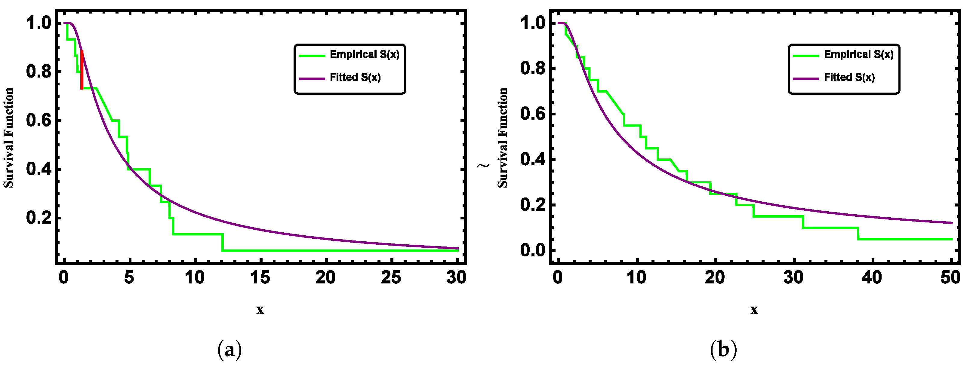
Since the p-values in

Table 1. Statistical measures for goodness-of-fit analysis of observed data.

Modes	A–D		C–M		Kuiper		K–S
	Statistic	p-Value	Statistic	p-Value	Statistic	p-Value	Statistic	p-Value
Dataset-I	0.4346	0.8101	0.0633	0.7925	0.2646	0.4331	0.2004	0.6982
Dataset-II	0.5394	0.7034	0.0865	0.6549	0.2298	0.4959	0.1673	0.7349

are greater than 0.05, the null hypothesis of the distribution cannot be rejected. This indicates that both datasets follow the G-II distribution, demonstrating the applicability of the proposed model to real data. To further illustrate this, Figure 3 presents the fitted and empirical survival functions of the G-II distribution for both datasets, showing strong agreement between them.

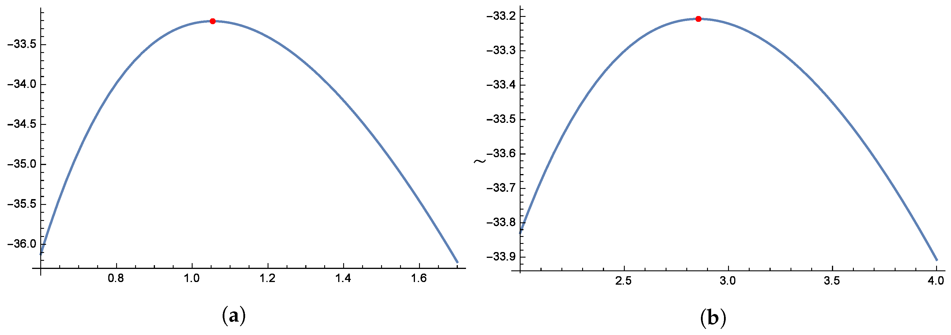
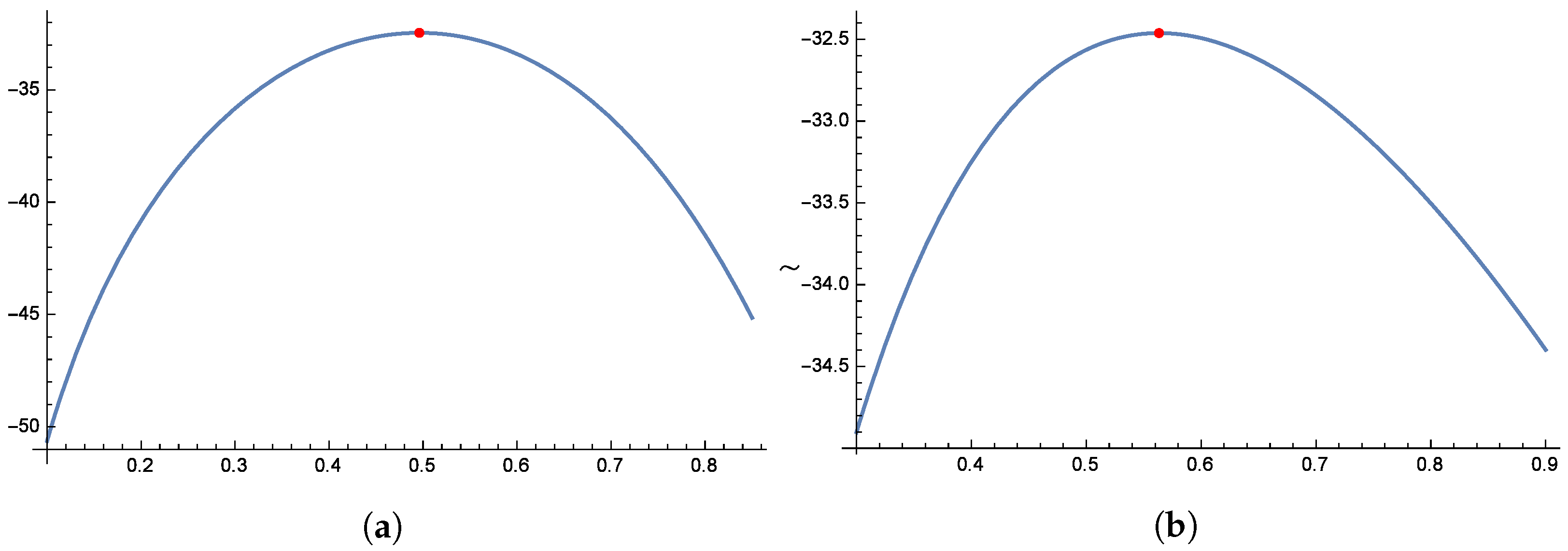
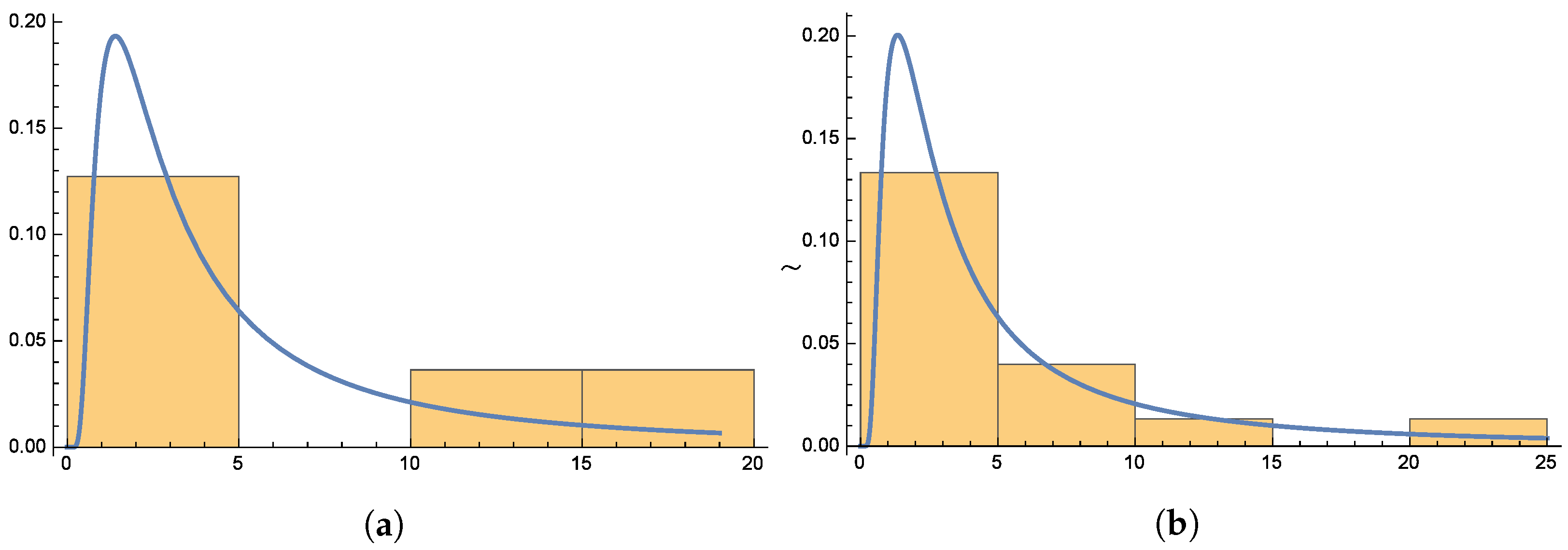
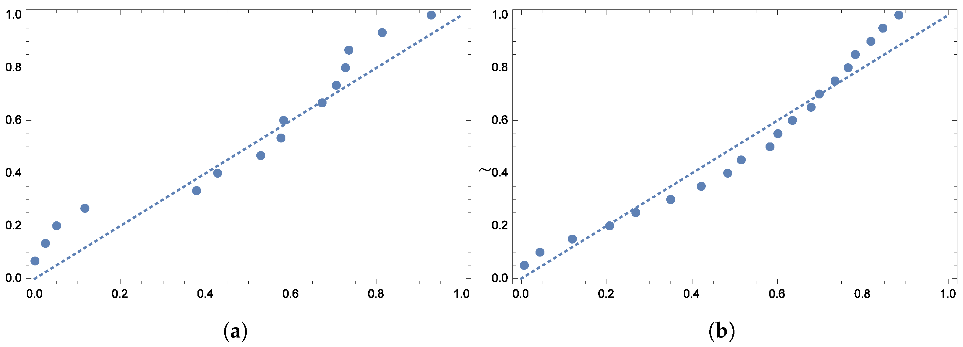
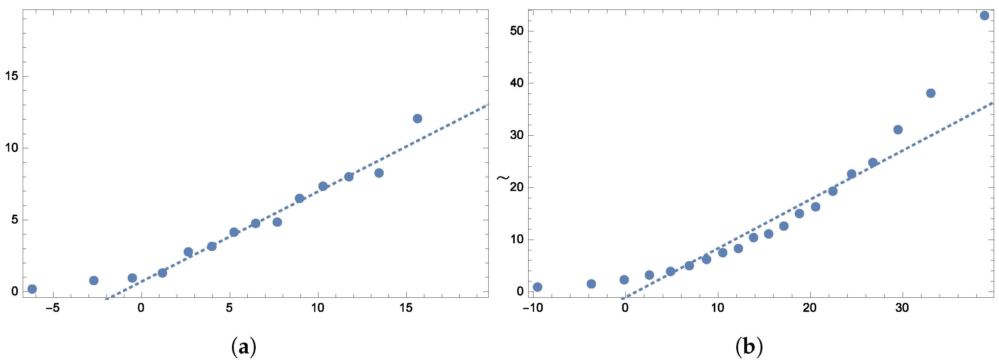
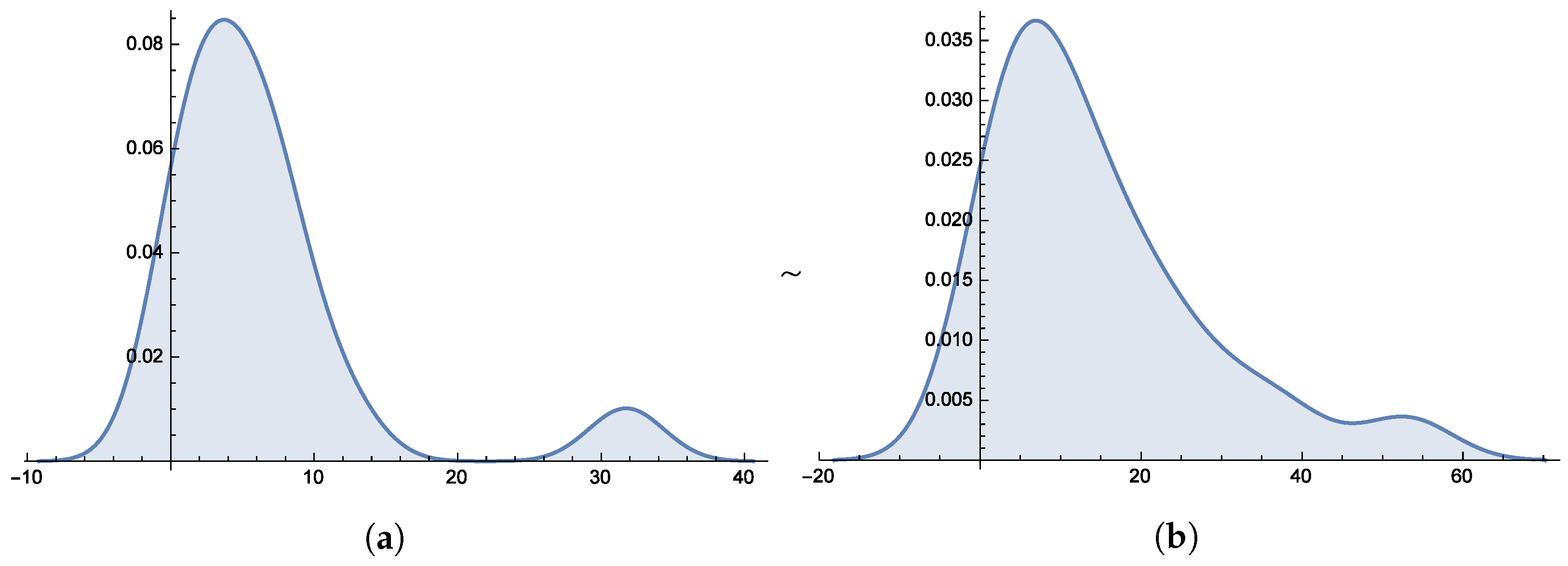
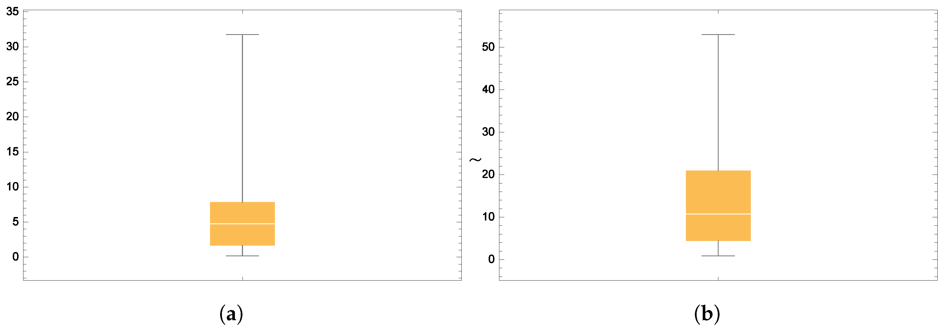
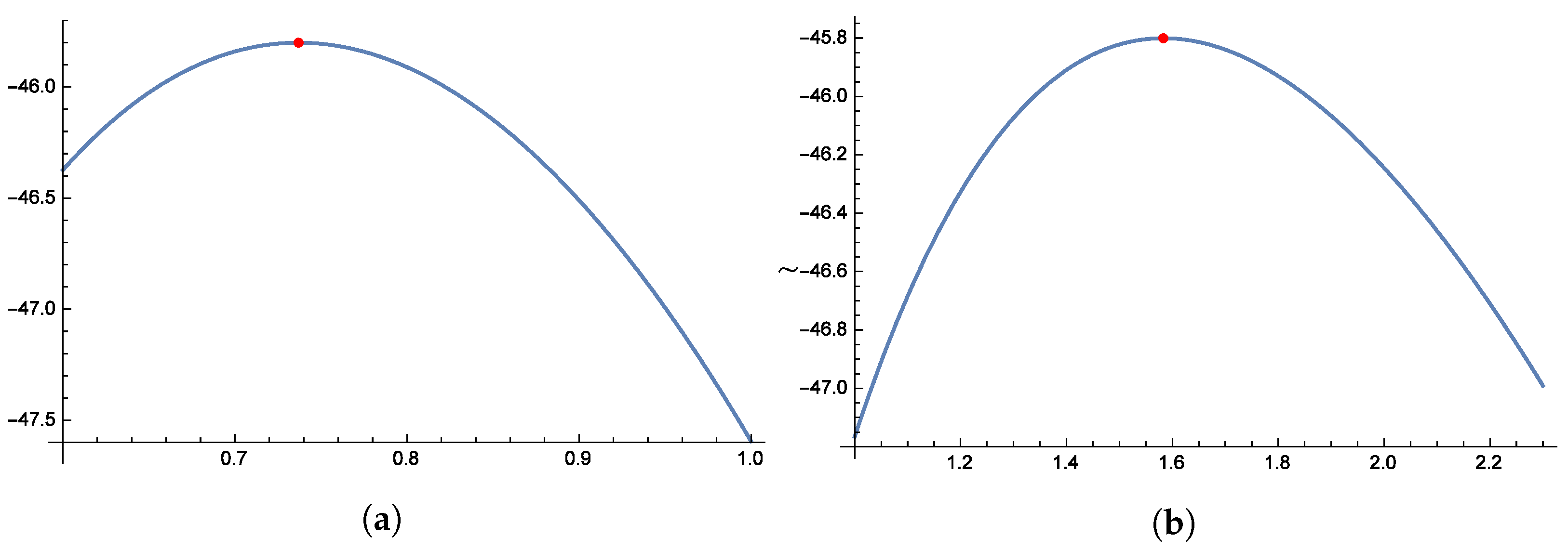
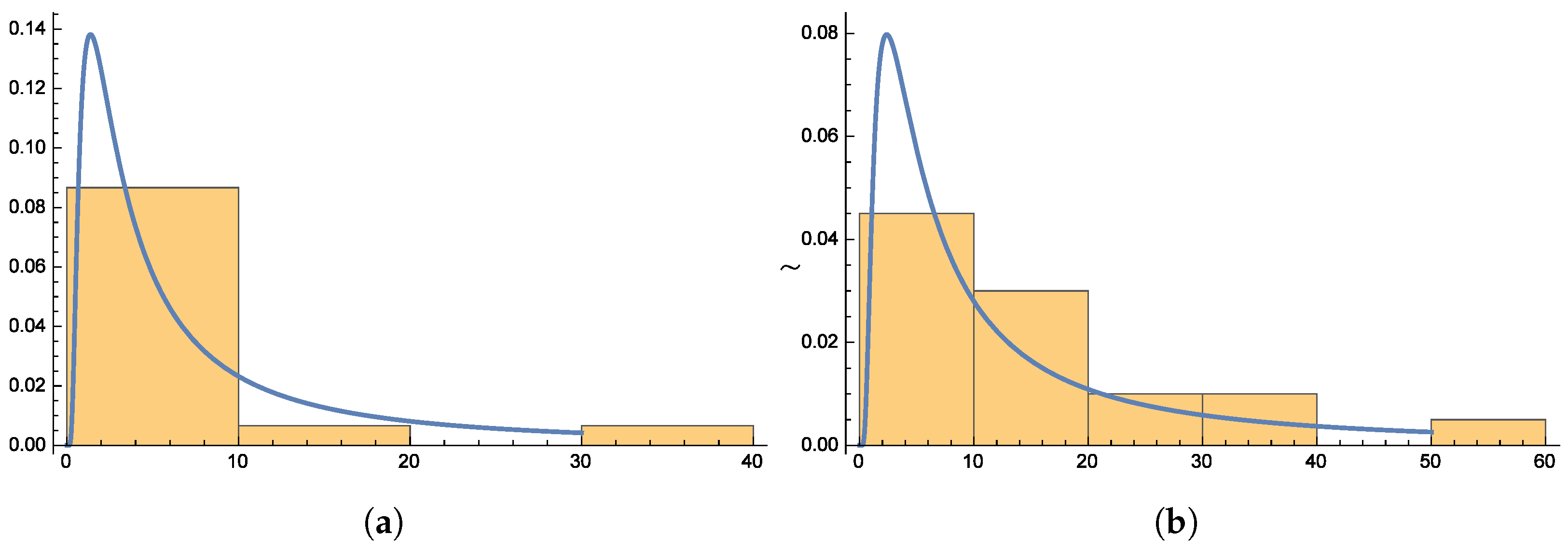
To further validate the model’s fit, Figure 4 and Figure 5 display the quantile plots and the observed versus expected probability plots, respectively. Figure 6 and Figure 7 present the smooth histogram and box-and-whisker chart for Dataset-I and Dataset-II. Figure 8 and Figure 9 illustrate the unimodal behavior of the profile log-likelihood function, which peaks within specific parameter ranges: 1.0 to 1.2 for ${\sigma }_1$, 2.5 to 3.5 for ${\theta }_1$, 0.4 to 0.6 for ${\sigma }_2$, and 0.5 to 0.7 for ${\theta }_2$. These distinct peaks confirm the existence of unique MLEs for ${\theta }_1$, ${\sigma }_1$, ${\theta }_2$, and ${\sigma }_2$. Finally, Figure 10 presents the histograms for both datasets, providing further evidence of the distribution’s suitability.

The censoring method outlined below was used to generate a Joint PCS sample based on the previously provided datasets. To perform Joint PCS with $r=10$, the first sample was set to $m=11$ and the second to $n=15$. The censoring vectors are defined as follows:

$$\begin{array}{c}\hfill \begin{array}{cc}\hfill S& =(0,0,0,0,0,0,0,0,0,6),\hfill \\ & R=(0,0,0,0,0,0,0,0,0,16),\hfill \\ & T=(0,0,0,0,0,0,0,0,0,10).\hfill \end{array}\end{array}$$

The datasets created are as follows:

$$\begin{array}{c}\hfill \begin{array}{cc}\hfill w& =(0.027,0.04,0.069,0.079,0.275,0.391,0.774,0.988,1.395,1.593),\hfill \\ & z=(0,0,0,0,0,0,1,0,0,0).\hfill \end{array}\end{array}$$

To determine estimates for ${\sigma }_1$, ${\sigma }_2$, ${\theta }_1$, and ${\theta }_2$, we used the MLE approach, depending on the type of data used in this study.

Table 2. MLE and Bayes estimates for $({\sigma }_1,{\sigma }_2,{\theta }_1,{\theta }_2)$.

Parameters	MLE	Bayes
		SEL	LINEX
			$\mathit{\epsilon }=-\mathbf{6.0}$	$\mathit{\epsilon }=\mathbf{0.00001}$	$\mathit{\epsilon }=\mathbf{6.0}$
${\sigma }_1$	0.6771	0.8955	0.8865	0.8844	0.8750
${\sigma }_2$	0.3623	0.5367	0.5252	0.5242	0.5232
${\theta }_1$	2.5611	2.0495	2.0411	2.0369	2.0253
${\theta }_2$	0.8840	1.1352	1.1231	1.1122	1.1112

displays the point estimates. While

Table 3. 95% CI and CRI for the parameters $({\sigma }_1,{\sigma }_2)$.

Method	${\mathit{\sigma }}_1$			${\mathit{\sigma }}_2$
	Lower	Upper	Length	Lower	Upper	Length
ACI	−0.4752	1.8294	2.3047	0.1787	0.5458	0.3671
CRI	0.89474	0.8959	0.0011	0.5365	0.5367	0.0002

and

Table 4. 95% CI and CRI for the parameters $({\theta }_1,{\theta }_2)$.

Method	${\mathit{\theta }}_1$			${\mathit{\theta }}_2$
	Lower	Upper	Length	Lower	Upper	Length
ACI	0.4156	4.7066	4.2910	0.3842	1.3836	0.9994
CRI	2.0494	2.0496	0.0002	1.1351	1.1356	0.0005

give the 95% ACIs for ${\sigma }_1$, ${\sigma }_2$, ${\theta }_1$, and ${\theta }_2$, We ran 10,000 iterations using the MCMC method for BE, excluding the first 2000 iterations as "burn-in" to guarantee convergence. For the previous distributions, the hyperparameters $a_i$ and $b_i$ that we have selected are ${10}^{-3}$, which is near zero. The corresponding point estimates are shown in Table 2. Bayesian estimates were constructed for ${\sigma }_1$, ${\sigma }_2$, ${\theta }_1$, and ${\theta }_2$ using both the SEL and LINEX loss functions. The 95% CRIs for ${\sigma }_1$, ${\sigma }_2$, ${\theta }_1$, and ${\theta }_2$ are also included in Table 3 and Table 4.

4.2. Example 2

This section presents a real dataset to illustrate the practical use of the proposed methods. The dataset was originally obtained from Zimmer et al. [36] and includes the following:

Data III Failure times (in hours) for 15 devices: 0.19, 0.78, 0.96, 1.31, 2.78, 3.16, 4.15, 4.76, 4.85, 6.5, 7.35, 8.01, 8.27, 12.06, 31.75.

Data IV First failure times (in months) for 20 electronic cards: 0.9, 1.5, 2.3, 3.2, 3.9, 5.0, 6.2, 7.5, 8.3, 10.4, 11.1, 12.6, 15.0, 16.3, 19.3, 22.6, 24.8, 31.5, 38.1, 53.0.

We applied several goodness-of-fit tests to evaluate the performance of the model, including the following

• A–D test.
• C–M test.
• Kuiper test.
• K–S test.

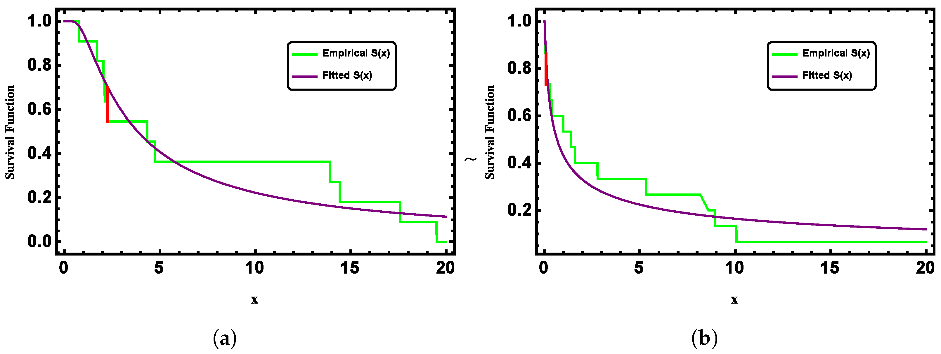
As the p-values in

Table 5. Statistical measures for goodness-of-fit analysis of observed data.

Modes	A–D		C–M		Kuiper		K–S
	Statistic	p-Value	Statistic	p-Value	Statistic	p-Value	Statistic	p-Value
Dataset-III	1.54062	0.167366	0.0862	0.6563	0.2121	0.6018	0.1500	0.8403
Dataset-IV	0.5607	0.6832	0.0869	0.6529	0.1992	0.5618	0.1331	0.8250

exceed 0.05, the null hypothesis cannot be rejected. This suggests that both datasets follow the G-II distribution, confirming the model’s applicability to real-world data. Figure 11 further supports this by comparing the fitted and empirical survival functions for both datasets, which show a strong alignment.

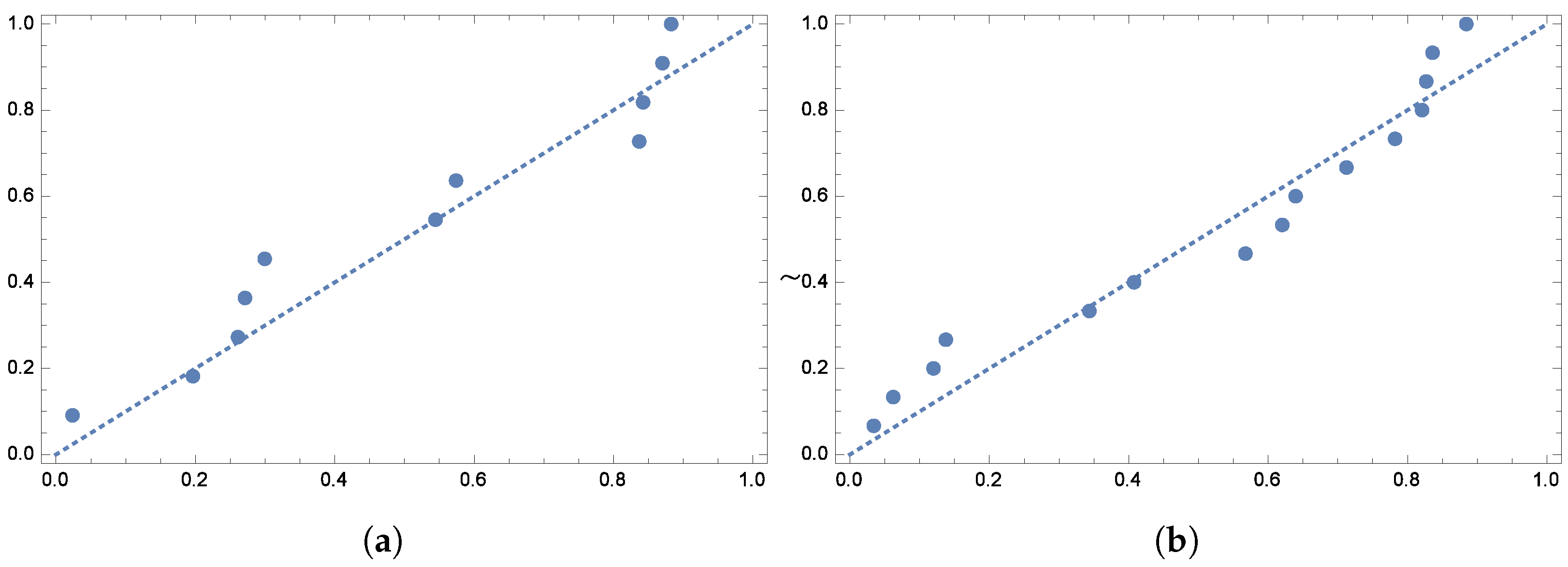
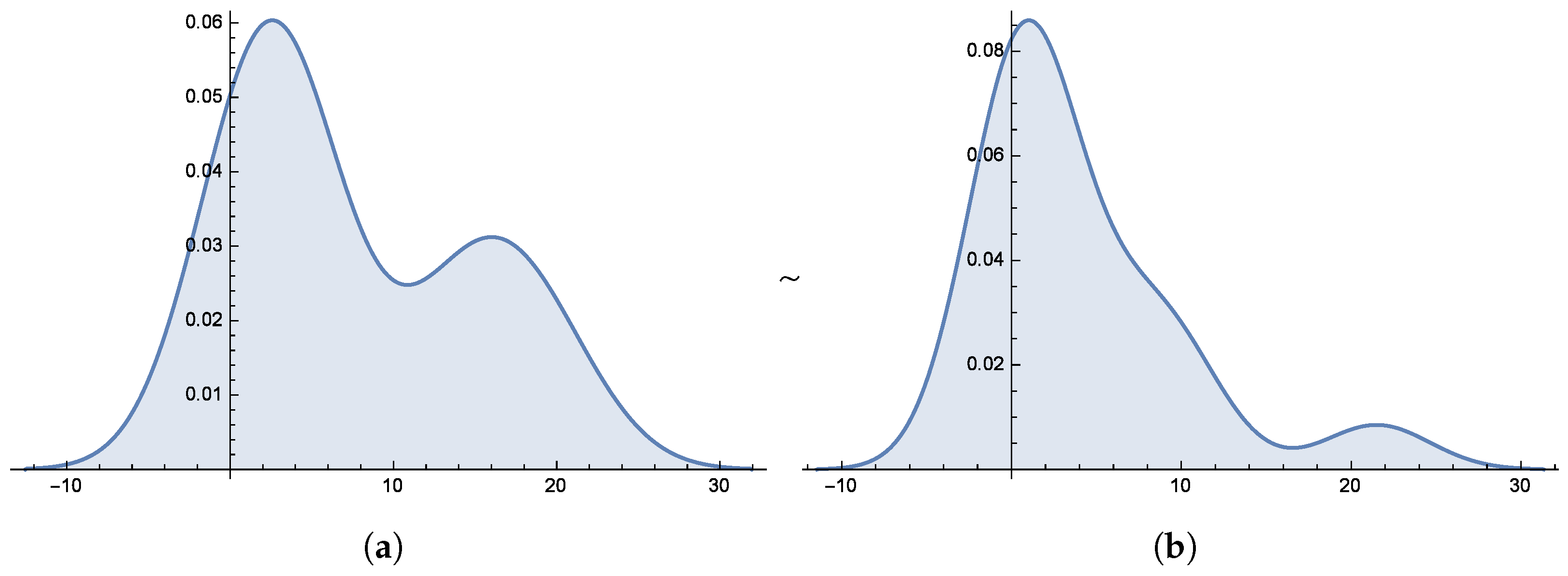
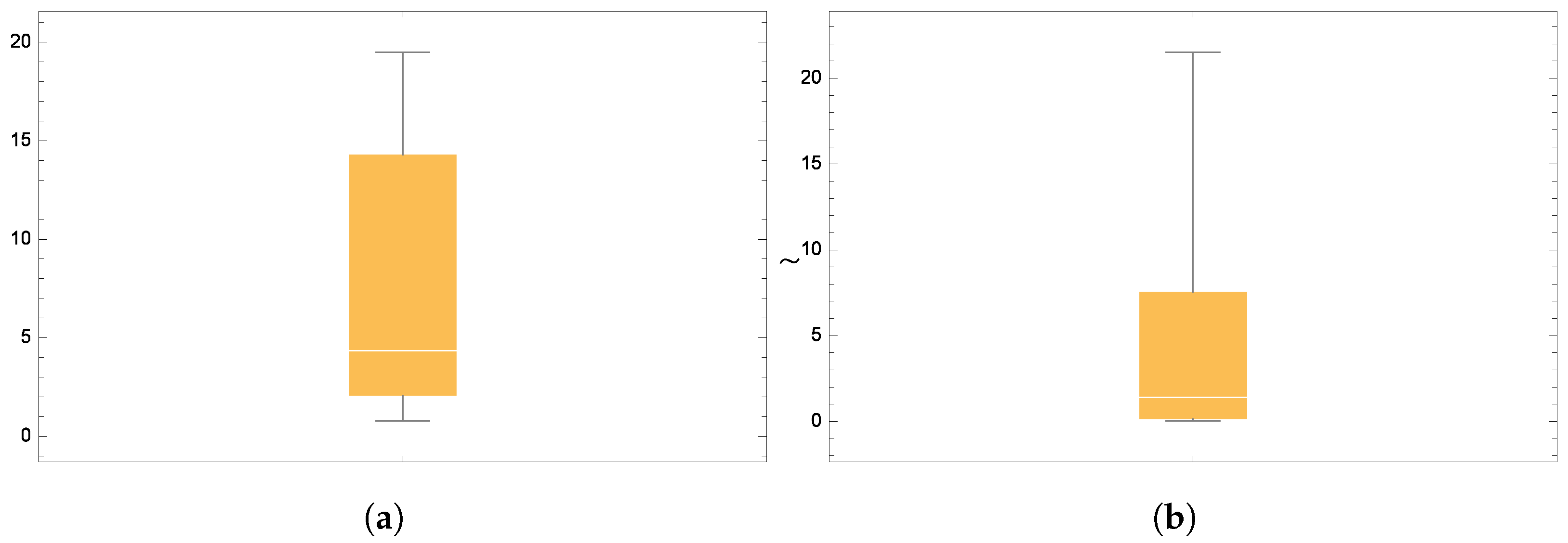
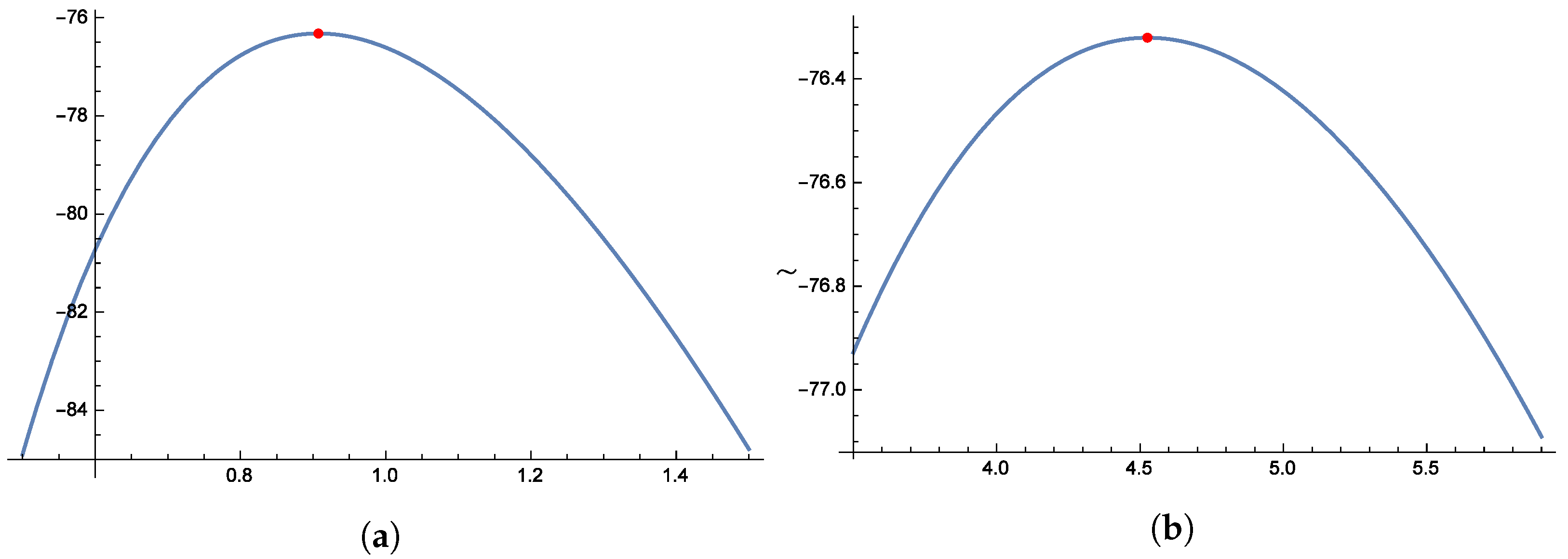
To further verify the model’s fit, Figure 12 and Figure 13 show the quantile plots and the observed versus expected probability plots. Figure 14 and Figure 15 display the smooth histograms and box-and-whisker plots for Dataset-III and Dataset-IV. Figure 16 and Figure 17 illustrate the unimodal shape of the profile log-likelihood functions, with peaks observed in the following parameter ranges: 0.7–0.8 for ${\sigma }_1$, 1.4–1.8 for ${\theta }_1$, 0.8–1.2 for ${\sigma }_2$, and 4.0–5.0 for ${\theta }_2$. These distinct peaks confirm the presence of unique maximum likelihood estimates for ${\theta }_1$, ${\sigma }_1$, ${\theta }_2$, and ${\sigma }_2$. Finally, Figure 18 presents the histograms of both datasets, offering additional evidence of the distribution’s suitability.

The censoring scheme described below was used to generate a joint PCS sample based on the previously provided datasets. To implement the joint PCS with $r=15$, the first sample size was set to $m=15$ and the second to $n=20$. The censoring vectors are specified as follows:

$$\begin{array}{c}\hfill \begin{array}{cc}\hfill S& =(0,0,0,0,0,0,0,0,0,0,0,0,0,0,8),\hfill \\ & R=(0,0,0,0,0,0,0,0,0,0,0,0,0,0,20),\hfill \\ & T=(0,0,0,0,0,0,0,0,0,0,0,0,0,0,12).\hfill \end{array}\end{array}$$

The generated datasets are as follows:

$$\begin{array}{c}\hfill \begin{array}{cc}\hfill w& =(0.19,0.78,0.9,0.96,1.31,1.5,2.3,2.78,3.16,3.2,3.9,4.15,4.76,4.85,5),\hfill \\ & z=(1,1,0,1,1,0,0,1,1,0,0,1,1,1,0).\hfill \end{array}\end{array}$$

Estimates for ${\sigma }_1$, ${\sigma }_2$, ${\theta }_1$, and ${\theta }_2$ were obtained using the MLE method, depending on the data type used in this study.

Table 6. MLE and Bayes estimates for $({\sigma }_1,{\sigma }_2,{\theta }_1,{\theta }_2)$.

Parameters	MLE	Bayes
		SEL	LINEX
			$\mathit{\epsilon }=-\mathbf{3.0}$	$\mathit{\epsilon }=\mathbf{0.0001}$	$\mathit{\epsilon }=\mathbf{3.0}$
${\sigma }_1$	0.5631	0.4430	0.4431	0.4442	0.4433
${\sigma }_2$	0.7383	0.7620	0.7618	0.7619	0.7621
${\theta }_1$	1.8161	2.3171	2.3139	2.3133	2.3135
${\theta }_2$	3.6324	3.8268	3.8265	3.8266	3.8264

presents the corresponding point estimates, while

Table 7. 95% CI and CRI for the parameters $({\sigma }_1,{\sigma }_2)$.

Method	${\mathit{\sigma }}_1$			${\mathit{\sigma }}_2$
	Lower	Upper	Length	Lower	Upper	Length
ACI	0.2981	0.8280	0.5298	0.2853	1.1911	0.9057
CRI	0.4429	0.4434	0.0005	0.7617	0.7623	0.0006

and

Table 8. 95% CI and CRI for the parameters $({\theta }_1,{\theta }_2)$.

Method	${\mathit{\theta }}_1$			${\mathit{\theta }}_2$
	Lower	Upper	Length	Lower	Upper	Length
ACI	0.9428	2.6893	1.7464	1.3873	5.8774	4.4901
CRI	2.3167	2.3175	0.0007	3.8262	3.8268	0.0006

provide the 95% ACIs for these parameters. For the Bayesian estimation, we performed 12,000 MCMC iterations, discarding the first 3000 as burn-in to ensure convergence. The hyperparameters $a_i$ and $b_i$ were set to ${10}^{-3}$, close to zero, for the prior distributions. The results are summarized in Table 6. Bayesian estimates for ${\sigma }_1$, ${\sigma }_2$, ${\theta }_1$, and ${\theta }_2$ were obtained under both the SEL and LINEX loss functions. Table 7 and Table 8 also include the 95% CRIs for these parameters.

To further validate the applicability of the proposed model, we conducted an in-depth analysis using the newly added datasets. The evaluation included multiple goodness-of-fit tests, such as the A–D, C–M, K–S, and Kuiper tests. In addition, graphical diagnostics were used, including fitted versus empirical survival functions, quantile plots, and probability plots. The analysis results confirmed that the proposed Gumbel Type-II model under joint progressive censoring provides improved fitting accuracy and narrower CRIs when compared with classical estimation methods. These findings support the practical advantages of the proposed approach in modeling lifetime and reliability data.

5. Simulation Study

This section evaluates the performance of the proposed estimation methods under Joint PCS using Monte Carlo simulations. The simulations were conducted using Mathematica version 10. The comparison focuses on point estimators for lifetime parameters based on the MSE:

$$\mathrm{MSE}\left(\widehat{\Theta }\right)={\displaystyle \frac{{\sum }_{i=1}^{1000}{({\Theta }_i-\widehat{\Theta })}^2}{1000}}.$$

A lower MSE indicates improved estimation accuracy. All results are based on 1000 replications. Additionally, average confidence lengths (ACLs) are examined, where a smaller ACL suggests better interval estimation performance. We selected two distinct censoring schemes, detailed below, for different failure counts ($r=15,20,25,35,40,50$) and sample sizes ($m=15,30,40$; $n=20,40,60$).

• Scheme I: $R_1=R_2=\cdots =R_{m-1}=0$ and $R_m=n-m$.
• Scheme II: $R_1=n-m$ and $R_2=R_3=\cdots =R_{m-1}=0$.

The parameter values for both datasets are ${\sigma }_1=1.5$, ${\sigma }_2=2.5$, ${\theta }_1=1.5$, and ${\theta }_2=2.5$. We computed the MLEs and 95% confidence intervals for ${\sigma }_1$, ${\sigma }_2$, ${\theta }_1$, and ${\theta }_2$. The mean values of the MLEs and their corresponding confidence interval lengths were determined after 1000 repetitions. The results are presented in

Table 9. (Non-) Bayesian estimates for the parameter ${\theta }_1$ are presented with their associated interval lengths and corresponding MSEs (shown in parentheses) for each censoring scheme.

$(\mathit{n},\mathit{m})$	r	Scheme	Non-Bayesian		Bayesian
			MLE	Length	SEL	LINEX		Length
						$\mathit{\epsilon }=-\mathbf{6.0}$	$\mathit{\epsilon }=\mathbf{6.0}$
(20, 15)	15	I	1.6084	1.4635	1.9269	1.9276	1.9263	0.3445
			(0.5117)		(0.1823)	(0.1829)	(0.1817)
	15	II	0.9592	1.3668	1.6625	1.6847	1.6379	0.2843
			(0.4924)		(0.1264)	(0.1261)	(0.1256)
(20, 15)	20	I	1.3605	1.2461	1.6499	1.6759	1.6213	0.2775
			(0.4195)		(0.1225)	(0.1232)	(0.1222)
	20	II	1.7207	1.2356	2.6959	2.7921	2.5759	0.2503
			(0.3887)		(0.1219)	(0.1214)	(0.1201)
(40, 30)	25	I	1.4244	0.9497	1.0638	1.0675	1.0597	0.1146
			(0.3057)		(0.1203)	(0.1187)	(0.1139)
	25	II	2.3456	2.8587	0.7612	0.8702	0.6795	0.2492
			(0.2715)		(0.1183)	(0.1098)	(0.1058)
(40, 30)	35	I	1.3074	0.9765	1.2671	1.2688	1.2655	0.1905
			(0.2371)		(0.1079)	(0.1044)	(0.1024)
	35	II	1.2406	1.1871	1.3266	1.3293	1.3238	0.1800
			(0.2273)		(0.0987)	(0.0975)	(0.0954)
(60, 40)	40	I	1.5542	1.0459	1.8465	1.8469	1.8461	0.1754
			(0.2029)		(0.0954)	(0.0954)	(0.0912)
	40	II	1.4427	1.1912	1.2979	1.3079	1.2875	0.1654
			(0.1985)		(0.0458)	(0.0452)	(0.0362)
(60, 40)	50	I	1.4838	0.9309	1.2828	1.2859	1.2794	0.1585
			(0.1875)		(0.0412)	(0.0411)	(0.0310)
	50	II	1.2199	0.9232	0.9069	0.9134	0.8995	0.1521
			(0.1560)		(0.0251)	(0.0223)	(0.0211)

,

Table 10. (Non-) Bayesian estimates for the parameter ${\theta }_2$ are presented with their associated interval lengths and corresponding MSEs (shown in parentheses) for each censoring scheme.

$(\mathit{m},\mathit{n})$	r	Scheme	Non-Bayesian		Bayesian
			MLE	Length	SEL	LINEX		Length
						$\mathit{\epsilon }=-\mathbf{6.0}$	$\mathit{\epsilon }=\mathbf{6.0}$
(20, 15)	15	I	5.7710	9.7029	6.7954	7.0503	4.7627	2.6867
			(2.6991)		(1.4506)	(1.4050)	(1.1197)
	15	II	6.4384	5.7124	4.5516	4.5512	4.5411	2.2046
			(1.1269)		(1.1092)	(1.1088)	(1.1010)
(20, 15)	20	I	3.0795	3.4908	3.4936	3.4936	3.4936	1.6985
			(0.8358)		(0.5872)	(0.5741)	(0.5633)
	20	II	4.0218	2.1976	6.8997	6.8995	6.6954	1.3280
			(0.5157)		(0.3572)	(0.3421)	(0.3410)
(40, 30)	25	I	2.4029	1.8423	2.9380	2.2263	2.7550	0.6685
			(0.4094)		(0.3112)	(0.125)	(0.3110)
	25	II	1.9033	1.6478	2.1290	2.9699	1.2844	0.62022
			(0.3560)		(0.3056)	(0.2593)	(0.2776)
(40, 30)	35	I	2.3505	1.5502	2.3035	2.3340	1.3733	0.4392
			(0.3224)		(0.2386)	(0.2276)	(0.2695)
	35	II	2.8469	1.5351	2.1712	2.3805	1.2798	0.4093
			(0.2204)		(0.2199)	(0.2181)	(0.2088)
(60, 40)	40	I	2.1920	1.1448	1.5169	1.5479	1.3955	0.3292
			(0.2549)		(0.2068)	(0.2011)	(0.1965)
	40	II	2.5244	1.1117	1.2239	1.3002	1.4930	0.3258
			(0.1854)		(0.1432)	(0.1365)	(0.1221)
(60, 40)	50	I	3.0745	1.0014	2.1366	2.1320	2.1125	0.3014
			(0.1785)		(0.1321)	(0.1311)	(0.1254)
	50	II	3.1202	1.0010	2.0984	2.8174	1.4298	0.2903
			(0.1658)		(0.1246)	(0.1252)	(0.1250)

,

Table 11. (Non-) Bayesian estimates for the parameter ${\sigma }_1$ are presented with their associated interval lengths and corresponding MSEs (shown in parentheses) for each censoring scheme.

$(\mathit{m},\mathit{n})$	r	Scheme	Non-Bayesian		Bayesian
			MLE	Length	SEL	LINEX		Length
						$\mathit{\epsilon }=-\mathbf{6.0}$	$\mathit{\epsilon }=\mathbf{6.0}$
(20, 15)	15	I	1.1904	1.1792	1.7127	1.4508	1.5189	0.6262
			(0.7792)		(0.3698)	(0.3654)	(0.3421)
	15	II	1.8472	1.0069	1.1445	1.2444	1.3539	0.5939
			(0.7206)		(0.2827)	(0.2814)	(0.2749)
(20, 15)	20	I	1.7716	1.4521	1.3945	1.3993	1.0231	0.4276
			(0.6737)		(0.2452)	(0.2421)	(0.2369)
	20	II	1.4137	1.4134	1.8666	1.2327	1.2516	0.4177
			(0.5574)		(0.2337)	(0.2329)	(0.2258)
(40, 30)	25	I	1.3128	1.0120	1.7053	1.3147	1.1884	0.4122
			(0.5218)		(0.2298)	(0.2244)	(0.2236)
	25	II	1.5758	1.2926	1.4152	1.3223	1.5572	0.3987
			(0.2126)		(0.1995)	(0.1888)	(0.1176)
(40, 30)	35	I	1.3606	1.0629	1.5859	1.4140	1.7215	0.3158
			(0.1994)		(0.1384)	(0.1654)	(0.1123)
	35	II	1.4462	1.0906	1.6554	1.3353	1.6833	0.2496
			(0.1779)		(0.1079)	(0.1054)	(0.1025)
(60, 40)	40	I	1.3571	1.1578	1.7165	1.4014	1.3079	0.2215
			(0.1564)		(0.0964)	(0.0932)	(0.0929)
	40	II	1.4066	1.0223	1.8079	1.2263	1.8775	0.2156
			(0.1426)		(0.0864)	(0.0845)	(0.0810)
(60, 40)	50	I	1.5750	0.9593	1.6747	1.4209	1.3221	0.2145
			(0.1354)		(0.0123)	(0.0121)	(0.0112)
	50	II	1.2473	0.8020	1.0935	1.3269	1.8507	0.2011
			(0.1236)		(0.0114)	(0.0110)	(0.0089)

and

Table 12. (Non-) Bayesian estimates for the parameter ${\sigma }_2$ are presented with their associated interval lengths and corresponding MSEs (shown in parentheses) for each censoring scheme.

$(\mathit{m},\mathit{n})$	r	Scheme	Non-Bayesian		Bayesian
			MLE	Length	SEL	LINEX		Length
						$\mathit{\epsilon }=-\mathbf{6}.\mathbf{0}$	$\mathit{\epsilon }=\mathbf{6}.\mathbf{0}$
(20, 15)	15	I	4.8712	5.4443	5.4383	5.5541	4.1223	4.6096
			(0.6227)		(0.5637)	(0.5624)	(0.4096)
	15	II	4.8177	3.5947	5.5393	5.2884	4.9038	4.0509
			(0.5655)		(0.3373)	(0.3996)	(0.3195)
(20, 15)	20	I	5.7156	3.5646	6.1677	5.4956	3.7353	3.5691
			(0.4465)		(0.3231)	(0.3125)	(0.2396)
	20	II	4.0839	3.0552	5.0408	5.2383	5.9063	2.9548
			(0.3731)		(0.2556)	(0.2315)	(0.2149)
(40, 30)	25	I	2.6930	2.4775	2.0491	2.6319	2.9109	2.7726
			(0.3373)		(0.1903)	(0.1945)	(0.1864)
	25	II	2.6852	1.7497	1.3210	1.2650	1.1965	1.5091
			(0.3215)		(0.1865)	(0.1823)	(0.1895)
(40, 30)	35	I	2.3404	1.5220	1.4873	1.5317	5.2177	0.2865
			(0.2954)		(0.1564)	(0.1452)	(0.1266)
	35	II	2.0133	1.0137	1.9689	1.2226	1.8171	0.2254
			(0.2548)		(0.1369)	(0.1364)	(0.1124)
(60, 40)	40	I	3.2673	1.9053	1.0482	1.6244	1.5626	0.2110
			(0.2487)		(0.1265)	(0.1264)	(0.1214)
	40	II	3.2736	1.0798	1.1569	1.2447	0.8470	0.2042
			(0.2321)		(0.1540)	(0.1523)	(0.1139)
(60, 40)	50	I	2.6226	1.0850	1.7142	1.5540	1.0223	0.1982
			(0.2214)		(0.1258)	(0.1202)	(0.1054)
	50	II	2.4912	1.0234	1.3244	1.1122	1.0765	0.1101
			(0.1952)		(0.1162)	(0.1102)	(0.1001)

.

Additionally, within the BE framework under SEL and LINEX loss functions, we employed informative gamma priors for ${\alpha }_1$, ${\alpha }_2$, ${\gamma }_1$, and ${\gamma }_2$. The hyperparameters were set as $a_i=0.05$ and $b_i=0.07$ for $i=1,2,3,4$. The values $\epsilon =6$ and $\epsilon =-6$ represented overestimation and underestimation, respectively. Where

• $\epsilon =6$ adds a constant positive bias, modeling overestimation.
• $\epsilon =-6$ adds a constant negative bias, modeling underestimation.

These shifts test how the estimator performs when the data is systematically too high or too low.

Using the MCMC approach, we obtained Bayesian estimates with 95% CRIs for ${\sigma }_1$, ${\sigma }_2$, ${\theta }_1$, and ${\theta }_2$ based on 1000 simulations with 21,000 samples. The initial 5000 iterations were discarded as a "burn-in" phase to ensure convergence. The performance of the obtained estimators for ${\sigma }_1$, ${\sigma }_2$, ${\theta }_1$, and ${\theta }_2$ was evaluated using MSE. After 1000 repetitions, we computed the mean values of the MLEs and their respective lengths. The results are presented in Table 9, Table 10, Table 11 and Table 12.

Here are the key findings from the manuscript:

• BE methods generally outperform classical MLE, particularly in terms of MSE and interval estimation precision.
• Joint PCS is shown to be an effective strategy for balancing cost and time while maintaining estimation accuracy.
• Bayesian estimators provide shorter CRIs compared with ACIs, making them more precise in uncertainty quantification.
• The LINEX loss function results in more efficient Bayesian estimators compared with the SEL function.
• The proposed methods effectively model real-world failure data, validating their use in reliability analysis.
• Extensive Monte Carlo simulations confirm that Bayesian estimates exhibit lower MSE and narrower CRIs, especially when informative priors are used.
• The M–H algorithm successfully approximates complex posterior distributions, ensuring efficient parameter estimation.

6. Conclusions

This study investigates estimating unknown parameters of the G-II distribution under joint progressive censoring using classical and Bayesian methods. It develops and compares estimation techniques, evaluates performance through simulations, and applies them to real data. Classical estimation uses maximum likelihood estimation for point estimates and approximate confidence intervals to measure uncertainty, showing that estimates improve with larger samples. Due to the complex likelihood, numerical methods are needed for parameter estimation. BE applies MCMC, specifically Metropolis–Hastings, to approximate posterior distributions, incorporating squared error and LINEX loss functions to compute Bayes estimators and obtain highest posterior density intervals. Simulations reveal that Bayesian methods generally yield lower mean squared errors and more precise intervals than classical methods by using prior information. Monte Carlo simulations compare estimation methods under different censoring schemes and parameter values, showing that increasing sample size reduces mean squared error and improves estimate precision, with Bayesian credible intervals shorter than classical intervals. Analysis of a real dataset demonstrates practical use of the proposed methods, confirming that joint progressive censoring effectively models failure data with cost and time benefits and that BE provides more robust results, especially with informative priors. The study improves statistical inference for extreme value distributions by refining parameter estimation under joint progressive censoring and highlights choosing estimation methods based on data and goals, suggesting future research apply these approaches to other heavy-tailed distributions, explore flexible priors, and enhance computational techniques for high-dimensional problems.

References

1. Gumbel, E. Statistics of Extremes; Columbia University Press: New York, NY, USA, 1958. [Google Scholar]
2. Mousa, M.A.; Jaheen, Z.; Ahmad, A. Bayesian estimation, prediction and characterization for the Gumbel model based on records. Stat. J. Theor. Appl. Stat. 2002, 36, 65–74. [Google Scholar] [CrossRef]
3. Malinowska, I.; Szynal, D. On a family of Bayesian estimators and predictors for a Gumbel model based on the kth lower records. Appl. Math. 2004, 1, 107–115. [Google Scholar] [CrossRef]
4. Miladinovic, B.; Tsokos, C.P. Ordinary, Bayes, empirical Bayes, and non-parametric reliability analysis for the modified Gumbel failure model. Nonlinear Anal. Theory Methods Appl. 2009, 71, e1426–e1436. [Google Scholar] [CrossRef]
5. Nadarajah, S.; Kotz, S. The beta Gumbel distribution. Math. Probl. Eng. 2004, 2004, 323–332. [Google Scholar] [CrossRef]
6. Feroze, N.; Aslam, M. Bayesian Analysis Of Gumbel Type II Distribution Under Doubly Censored Samples Using Different Loss Functions. Casp. J. Appl. Sci. Res. 2012, 1, 26–43. [Google Scholar]
7. Abbas, K.; Fu, J.; Tang, Y. Bayesian estimation of Gumbel type-II distribution. Data Sci. J. 2013, 12, 33–46. [Google Scholar] [CrossRef]
8. Feroze, N.; Aslam, M. Bayesian estimation of twocomponent mixture of gumbel type II distribution under informative priors. Int. J. Adv. Sci. Technol. 2013, 53, 11–30. [Google Scholar]
9. Reyad, H.M.; Ahmed, S.O. E-Bayesian analysis of the Gumbel type-II distribution under type-II censored scheme. Int. J. Adv. Math. Sci. 2015, 3, 108–120. [Google Scholar] [CrossRef]
10. Sindhu, T.N.; Feroze, N.; Aslam, M. Study of the left censored data from the gumbel type II distribution under a bayesian approach. J. Mod. Appl. Stat. Methods 2016, 15, 10–31. [Google Scholar] [CrossRef]
11. Abbas, K.; Hussain, Z.; Rashid, N.; Ali, A.; Taj, M.; Khan, S.A.; Manzoor, S.; Khalil, U.; Khan, D.M. Bayesian estimation of gumbel type-II distribution under type-II censoring with medical applicatioNs. Comput. Math. Methods Med. 2020, 2020, 1876073. [Google Scholar] [CrossRef]
12. Qiu, Y.; Gui, W. Statistical Inference for Two Gumbel Type-II Distributions under Joint Type-II Censoring Scheme. Axioms 2023, 12, 572. [Google Scholar] [CrossRef]
13. Balakrishnan, N.; Aggarwala, R. Progressive Censoring: Theory, Methods, and Applications; Springer Science & Business Media: Berlin/Heidelberg, Germany, 2000. [Google Scholar]
14. Balakrishnan, N.; Cramer, E. The Art of Progressive Censoring; Statistics for Industry and Technology; Birkhsuser: Boston, MA, USA, 2014. [Google Scholar]
15. Balakrishnan, N.; Sandhu, R.A. A simple simulational algorithm for generating progressive Type-II censored samples. Am. Stat. 1995, 49, 229–230. [Google Scholar] [CrossRef]
16. Singh, K.; Kumar Mahto, A.; Mani Tripathi, Y.; Wang, L. Estimation in a multicomponent stress-strength model for progressive censored lognormal distribution. Proc. Inst. Mech. Eng. Part J. Risk Reliab. 2024, 238, 622–642. [Google Scholar]
17. Hasaballah, M.M.; Tashkandy, Y.A.; Balogun, O.S.; Bakr, M.E. Bayesian and Classical Inference of the Process Capability Index under Progressive Type-II Censoring Scheme. Phys. Scr. 2024, 99, 055241. [Google Scholar] [CrossRef]
18. Rasouli, A.; Balakrishnan, N. Exact Likelihood Inference for Two Exponential Populations Under Joint Progressive Type-II Censoring. Commun. Stat.-Theory Methods 2010, 39, 2172–2191. [Google Scholar] [CrossRef]
19. Pandey, R.; Srivastava, P. Bayesian inference for two log-logistic populations under joint progressive type II censoring schemes. Int. Syst. Assur. Eng. Manag. 2022, 13, 2981–2991. [Google Scholar] [CrossRef]
20. Qiao, Y.; Gui, W. Statistical Inference of Weighted Exponential Distribution under Joint Progressive Type-II Censoring. Symmetry 2022, 14, 2031. [Google Scholar] [CrossRef]
21. Abdel-Aty, Y.; Kayid, M.; Alomani, G. Generalized Bayes Estimation Based on a Joint Type-II Censored Sample from K-Exponential Populations. Mathematics 2023, 11, 2190. [Google Scholar] [CrossRef]
22. Long, B.; Jiang, Z. Estimation and prediction for two-parameter Pareto distribution based on progressively double Type-II hybrid censored data. AIMS Math. 2023, 8, 15332–15351. [Google Scholar] [CrossRef]
23. Ren, H.; Hu, X. Estimation for inverse Weibull distribution under progressive type-II censoring scheme. AIMS Math. 2023, 8, 22808–22829. [Google Scholar] [CrossRef]
24. Hu, X.; Ren, H. Statistical inference of the stress-strength reliability for inverse Weibull distribution under an adaptive progressive type-II censored sample. AIMS Math. 2023, 8, 28465–28487. [Google Scholar] [CrossRef]
25. Panahi, H. Reliability estimation and order-restricted inference based on joint type-II progressive censoring scheme with application to splashing data in atomization process. Proc. Inst. Mech. Eng. Part J. Risk Reliab. 2024, 239. [Google Scholar] [CrossRef]
26. Hasaballah, M.M.; Balogun, O.S.; Bakr, M.E. Non-Bayesian and Bayesian estimation for Lomax distribution under randomly censored with application. AIP Adv. 2024, 14, 025318. [Google Scholar] [CrossRef]
27. Hasaballah, M.M.; Tashkandy, Y.A.; Bakr, M.E.; Balogun, O.S.; Ramadan, D.A. Classical and Bayesian inference of inverted modified Lindley distribution based on progressive type-II censoring for modeling engineering data. AIP Adv. 2024, 14, 035021. [Google Scholar] [CrossRef]
28. Hasaballah, M.M.; Tashkandy, Y.A.; Balogun, O.S.; Bakr, M.E. Statistical Inference of Unified Hybrid Censoring Scheme for Generalized Inverted Exponential Distribution with Application to COVID-19 Data. AIP Adv. 2024, 14, 045111. [Google Scholar] [CrossRef]
29. Hasaballah, M.M.; Tashkandy, Y.A.; Oluwafemi Samson Balogun, O.S.; Bakr, M.E. Reliability analysis for two populations Nadarajah-Haghighi distribution under Joint progressive type-II censoring. AIMS Math. 2024, 9, 10333–10352. [Google Scholar] [CrossRef]
30. Hasaballah, M.M.; Balogun, O.S.; Bakr, M.E. Point and interval estimation based on joint progressive censoring data from two Rayleigh-Weibull distribution with applications. Phys. Scr. 2024, 99, 8. [Google Scholar] [CrossRef]
31. Hasaballah, M.M.; Balogun, O.S.; Bakr, M.E. Frequentist and Bayesian approach for the generalized logistic lifetime model with applications to air-conditioning system failure times under joint progressive censoring data. AIMS Math. 2024, 9, 29346–29369. [Google Scholar] [CrossRef]
32. Varian, H.R. A Bayesian approach to real state assessment. In Studies in Bayesian Econometrics and Statistics; In Honor of Leonard J. Savage; Stephen, E.F., Zellner, A., Eds.; North-Holland: Amsterdam, The Netherland, 1975; pp. 195–208. [Google Scholar]
33. Metropolis, N.; Rosenbluth, A.W.; Rosenbluth, M.N.; Teller, A.H.; Teller, E. Equation of State Calculations by Fast Computing. Mach. J. Chem. Phys. 1953, 21, 1087–1092. [Google Scholar] [CrossRef]
34. Hastings, W.K. Monte Carlo sampling methods using Markov chains and their applications. Biometrika 1970, 57, 97–109. [Google Scholar] [CrossRef]
35. Nelson, W.B. Accelerated Testing: Statistical Models, Test Plans, and Data Analysis; John Wiley & Sons: Hoboken, NJ, USA, 2009. [Google Scholar]
36. Zimmer, W.J.; Keats, J.B.; Wang, F.K. The Burr-XII distribution in reliability analysis. J. Qual. Technol. 1998, 30, 386–394. [Google Scholar] [CrossRef]
Figure 1. Illustrates the PDF of the G-II distribution for various σ values while keeping θ fixed.
Axioms 14 00544 g001
Figure 2. Illustrates the CDF of the G-II distribution for various σ values while keeping θ fixed.
Axioms 14 00544 g002
Figure 3. (a) Empirical and fitted survival function for Dataset-I. (b) Empirical and fitted survival function for Dataset-II.
Axioms 14 00544 g003
Figure 4. (a) Probability plot for Dataset-I. (b) Probability plot for Dataset-II.
Axioms 14 00544 g004
Figure 5. (a) Quantile plot for Dataset-I. (b) Quantile plot for Dataset-II.
Axioms 14 00544 g005
Figure 6. (a) Smooth histogram for Dataset-I. (b) Smooth histogram for Dataset-II.
Axioms 14 00544 g006
Figure 7. (a) Box whisker chart for Dataset-I. (b) Box whisker chart for Dataset-II.
Axioms 14 00544 g007
Figure 8. (a) Profile log-likelihood function of σ 1 for Dataset-I. (b) Profile log-likelihood function of θ 1 for Dataset-II.
Axioms 14 00544 g008
Figure 9. (a) Profile log-likelihood function of σ 2 for Dataset-I. (b) Profile log-likelihood function of θ 2 for Dataset-II.
Axioms 14 00544 g009
Figure 10. (a) Histogram for Dataset-I. (b) Histogram for Dataset-II.
Axioms 14 00544 g010
Figure 11. (a) Empirical and fitted survival function for Dataset-III. (b) Empirical and fitted survival function for Dataset-IV.
Axioms 14 00544 g011
Figure 12. (a) Probability plot for Dataset-III. (b) Probability plot for Dataset-IV.
Axioms 14 00544 g012
Figure 13. (a) Quantile plot for Dataset-III. (b) Quantile plot for Dataset-IV.
Axioms 14 00544 g013
Figure 14. (a) Smooth histogram for Dataset-III. (b) Smooth histogram for Dataset-IV.
Axioms 14 00544 g014
Figure 15. (a) Box whisker chart for Dataset-III. (b) Box whisker chart for Dataset-IV.
Axioms 14 00544 g015
Figure 16. (a) Profile log-likelihood function of σ 1 for Dataset-III. (b) Profile log-likelihood function of θ 1 for Dataset-IV.
Axioms 14 00544 g016
Figure 17. (a) Profile log-likelihood function of σ 2 for Dataset-III. (b) Profile log-likelihood function of θ 2 for Dataset-IV.
Axioms 14 00544 g017
Figure 18. (a) Histogram for Dataset-III. (b) Histogram for Dataset-IV.
Axioms 14 00544 g018