Abstract
Bayesian networks (BNs) are effective and universal tools for addressing uncertain knowledge. BN learning includes structure learning and parameter learning, and structure learning is its core. The topology of a BN can be determined by expert domain knowledge or obtained through data analysis. However, when many variables exist in a BN, relying only on expert knowledge is difficult and infeasible. Therefore, the current research focus is to build a BN via data analysis. However, current data learning methods have certain limitations. In this work, we consider a combination of expert knowledge and data learning methods. In our algorithm, the hard constraints are derived from highly reliable expert knowledge, and some conditional independent information is mined by feature selection as a soft constraint. These structural constraints are reasonably integrated into an exponential Monte Carlo with counter (EMCQ) hyper-heuristic algorithm. A comprehensive experimental study demonstrates that our proposed method exhibits more robustness and accuracy compared to alternative algorithms.
MSC:
68W25; 68Q07; 68R10; 05C90
1. Introduction
Bayesian networks are among the most effective methods for studying high-dimensional uncertainty problems and have been widely used in medicine [1,2], fault diagnosis [3], environmental protection [4], and other fields. When BN theory is used to solve practical problems, the graph model of causal relationships between variables must be established first.
Global and local structure learning are the two current classifications for Bayesian network structure learning methods. The global learning method is further subdivided into three primary categories: constraint-based methods, score-based methods, and hybrid methods. Conditional independence (CI) tests are the foundation of constraint-based methods, which are used to determine causal links. Both SGS and TPDA [5] determine the network structure by evaluating the conditional independence among nodes. However, the computational complexity of these two algorithms increases exponentially with the number of nodes, so they are not suitable for dealing with large networks. To mitigate the computing cost, the PC and PC-Stable algorithms [6,7] take advantage of the characteristic that nodes in sparse networks do not require high-order independence tests. They employ a reduction strategy to efficiently establish Bayesian networks from the sparse model. However, the small sample size leads to a decrease in the statistical power of the CI test and an increase in the estimation error. The score-based method regards structure learning as a combinatorial optimization problem. Its core lies in searching for the optimal solution in the possible structure space through the score function and the search algorithm. This method consists of two key components: the design of the scoring function and the optimization of the search strategy. Prevalent scoring functions encompass K2, the BIC, and the MDL, whereas typical search spaces consist of three types: the directed acyclic graph (DAG) space [8], which is composed of all possible directed acyclic graphs; the equivalence class space [9], which groups Markov equivalent DAGs into the same equivalence class; and the ordering space [10], which is based on the topological ordering of variables. There are two primary types of search strategies: approximate learning and exact learning. Exact learning [11,12,13,14] theoretically ensures strict convergence to the theoretical optimal solution, but the computational cost increases exponentially with the number of variables. Therefore, this method is practically unfeasible for large-scale datasets. In contrast, approximate learning algorithms sacrifice controllable accuracy in exchange for computational feasibility and are the preferred choice for high-dimensional and real-time scenarios. Approximate learning algorithms converge probabilistically. The quality of the solution is affected by the sampling quantity and the design of the algorithm. The earliest proposed algorithms, hill-climbing algorithm [5] and K2 [15], are based on the greedy search strategy and are prone to fall into local optima. Subsequently, a series of metaheuristic algorithms, such as the genetic algorithm (GA) [16], evolutionary programming [17], ant colony optimization (ACO) [18], cuckoo optimization (CO) [19], water cycle optimization (WCO) [20], particle swarm optimization (PSO) [21,22], artificial bee colony algorithm (ABC) [23], bacterial foraging optimization (BFO) [24], and firefly algorithm (FA) [25], have been proposed to improve search efficiency and escape local optima. Although these metaheuristic algorithms demonstrate exceptional efficacy in addressing real-world issues, two hurdles persist when confronted with complex and extensive networks:
- A single metaheuristic algorithm cannot assure optimal performance while learning various Bayesian networks.
- In the case of large-scale Bayesian networks, these metaheuristic algorithms often succumb to local optima, leading to diminished accuracy of the resulting graph.
Hybrid methods combine two classes of algorithms in an attempt to integrate the advantages of both. The search space of the score-based method is typically constrained by the constraint-based algorithm, with the most commonly used hybrid algorithm being the MMHC algorithm [26].
The core objective of the local learning method is to identify the local dependency structure of the target variable. This is specifically manifested in the discovery of two key sets of nodes: the parent–child set (PC) and the Markov blanket (MB). The GS [27] algorithm, through a two-stage framework of the growing stage (full coverage) and the shrinking phase (minimization refinement), has for the first time provided a theoretically complete guarantee for Markov boundary learning, becoming a landmark method in the field of causal feature selection. However, the local structure learning approach is dependent on CI tests, similar to the constrained global structure learning method, and its accuracy significantly decreases as the sample size decreases. The BAMB [28] method and the EEMB [29] algorithm achieve an optimal balance between data utility (covering real dependencies) and time cost (controlling the computational scale) through the dynamic alternation mechanism of PC learning and spouse learning. The F2SL [30] algorithm achieves the coordinated optimization of causal discovery efficiency and accuracy through the process of feature selection, skeleton construction, and direction determination. LCS-FS [31] uses mutual information as a proxy for causal correlation measurement. By eliminating the condition set and incorporating a dynamic pruning mechanism, it significantly improves efficiency.
In conclusion, each method has distinct limitations and advantages. The core challenge currently faced in Bayesian network structure learning lies in how to achieve a deep synergy among different methodologies. Such as the integration strategy of constraints and scoring methods, the collaborative mechanism of global and local learning, and the enhancement of theoretical complementarity. This is the focus of this paper’s research. Hyper-heuristics have been employed across various domains to supplant metaheuristics because of their superior generalization capability and precision [32,33,34,35]. We explore the application of hyper-heuristics in lieu of metaheuristics for global structure learning.
The main contributions of this article are as follows:
- A feature selection-based method for MB discovery was employed to construct the search space and direction determination, and this knowledge served as soft constraints.
- We develop a library of low-level operations for BN structure learning.
- We propose an Exponential Monte Carlo with counter hyper-heuristic (EMCQ-HH) algorithm that integrates the soft and hard constraints derived from local structure learning techniques.
The subsequent sections of this article are structured as follows. Background information and associated concepts are introduced in Section 2. The study’s research design is described in Section 3. The performance evaluation and experimental findings are covered in Section 4. This work is concluded with some observations and recommendations for further research in Section 5.
2. Background
This section first introduces the DAG structure for discrete data through a BN and presents some basic properties and theorems of the DAG structure. This introduces the information theory basis for feature selection.
2.1. BN
Bayesian networks are a type of probabilistic graphical model. They represent the conditional dependencies among random variables through a directed acyclic graph and perform quantitative modeling on the basis of conditional probability distributions. A Bayesian network can be denoted as a two-tuple , where G denotes a DAG and signifies the set of conditional probability distributions. As a DAG, G can be described as a two-tuple , where represents the set of nodes, and each node corresponds to a variable. E represents the set of directed edges, and each edge denotes the dependency relationship between two nodes. The BN parameter is a distribution, which is manifested as a series of factorizations on the graph G.
where represents the conditional probability of when its parent node is given. Each node in has directed edges pointing to . Figure 1 shows a simple BN structure in which nodes X and Y are both parent nodes of node Z. These three variables form a simple V-structure, and their conditional probability tables are shown in the figure.
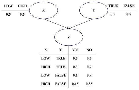
Figure 1.
A simple BN structure.
For discrete variables X, Y, and Z, when and only when the joint probability distribution can be expressed as the product of the conditional marginal distributions:
X and Y are conditionally independent given Z. The independence test can be characterized by the statistic and mutual information to depict the dependence and independence relationships between variables. For the two discrete variables X and Y, if the independence condition holds, then the statistic
approximately follows a -distribution with degree of freedom. For the three discrete variables X, Y and Z, if the independence condition holds, then the statistic
approximately follows a -distribution with degrees of freedom. In the above definition, , , and represent the number of possible values for X, Y, and Z, respectively.
2.2. Information Theory
Entropy is the core metric in information theory used to quantify the uncertainty of a random variable X. Its calculation formula is
The mutual information is a key metric in information theory for quantifying the shared information between two random variables X and Y. It measures the statistical dependence between the variables through the difference in probability distributions, and the calculation formula is
Conditional mutual information quantifies the remaining dependence or shared information between two variables X and Y, given a third random variable Z. The calculation formula is
2.3. Scoring Function
The BIC scoring function in Bayesian networks is the core indicator for evaluating the quality of the network structure. Its goal is to strike a balance between goodness of fit and model complexity. The formula is defined as
where g represents the network that requires scoring calculation, D denotes the training set, indicates the maximum likelihood estimator, m represents the sample size, and is equal to the dimension value of .
3. Methodology
The proposed method is a combined strategy based on constraint-based and score-based algorithms. With respect to the constraint-based part, we employed the WLBRC [36] algorithm to extract conditional independence information, thereby establishing three restricted search spaces (,,) and identifying partial edges. The identified edges and search spaces act as soft constraints, whereas hard constraints are provided by expert knowledge. With respect to the score-based part, soft and hard constraints are incorporated into our proposed hyper-heuristic algorithm as structural constraints.
3.1. Proposed Hyper-Heuristic Algorithm
The hyper-heuristic algorithm can be divided into two main parts: a high-level selection strategy and a low-level heuristic operator library. For the Bayesian network structure learning problem, we assemble a set of low-level heuristic operators with different functions by referring to the proposed metaheuristic algorithm and consider a simple parameter-free EMCQ method [35] for the high-level strategy. Figure 2 shows the framework of the proposed EMCQ-HH algorithm.
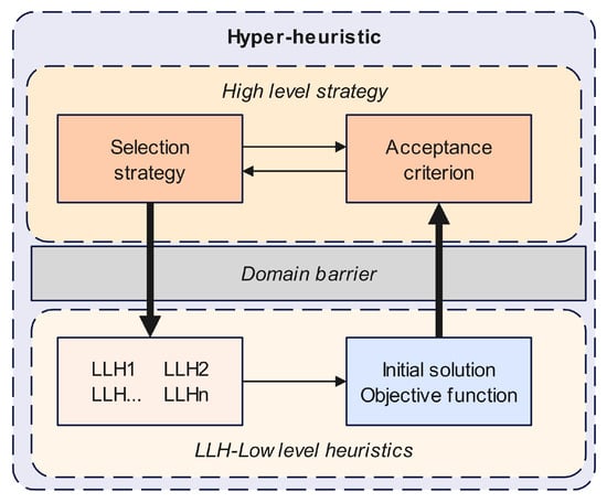
Figure 2.
Framework of the proposed EMCQ-HH algorithm.
In our work, EMCQ is similar to the simulated annealing method, where the probability density is defined as
where T is the number of current iterations and q is the control parameter for the diversity of the selection operator. The pseudocode of the EMCQ-HH algorithm is illustrated in Algorithm 1. The initial population starts with all edges identified by the hard and soft constraints, followed by multiple hill-climbing operations on to optimize the initial structure and generate the initial population. At the beginning of the iteration, an operator is randomly selected to update the population, and then the operator continues to be selected if the global optimal score is improved. If the global optimal score does not increase, the probability density function is computed, and a random number between 0 and 1 is generated. If the random number is less than , the operator is retained; otherwise, a new operator is randomly selected. Finally, the algorithm stops when a local optimal solution is reached or the maximum number of iterations is reached.
| Algorithm 1: EMCQHH |
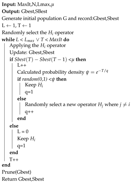 |
3.2. Low-Level Heuristics
By analyzing various heuristic algorithms for Bayesian network structure learning, we extract two mutation operators, three neighborhood hill-climbing operators, four learning operators, two restart operators, and expert knowledge operators to construct the underlying operator library. In addition, to better integrate expert knowledge and structural priors, we have made appropriate modifications to the underlying operators.
3.2.1. Mutation Operators
The two mutation operators extracted are the mutation operator and the neighborhood search operator. The former is extracted from a classical Bayesian network structure learning particle swarm algorithm [22], whereas the latter is a perturbation operator commonly used in combinatorial optimization problems. The former contains only one mutation operator, whereas the latter contains three operators: add, delete, and reverse.
3.2.2. Neighborhood Hill-Climbing Operators
The three neighborhood hill-climbing operators extracted are the chemotactic operator, employed bees, and onlooker bees. The chemotactic operator is extracted from a bacterial foraging optimization algorithm [24] applied to Bayesian network structure learning but does not consider the exchange operation. The operator operates on only one node at a time, greedily choosing to add, remove, or reverse edges for continuous operation. The last two operators are extracted from an artificial bee colony optimization algorithm [23] applied to BN structure learning, and they use different strategies to select an individual for climbing operations.
3.2.3. Learning Operators
The four learning operators extracted are the cognitive personal operator, cooperative global operator, moth-flame optimization, and teaching-learning-based optimization. The cognitive personal operator and cooperative global operator are extracted from the same particle swarm optimization algorithm [22] applied to Bayesian network structure learning, whose learning objects are individual historical optimal and global optimal, respectively. Moth-flame optimization randomly selects the historically optimal structure of an individual as a flame and learns from it. The teaching-learning-based optimization operator randomly selects an individual as its collaborator and learns from it if it is better than itself.
3.2.4. Restart Operators
The elimination and dispersal operator, derived from the bacterial foraging optimization method [24], is one component. Another component is scout bees [23], derived from an artificial bee colony optimization method. For large Bayesian networks, blindly rebooting new structures may be inefficient for escaping local optima. Therefore, we consider local restarts on a globally optimal structure, which only changes the local structure of one node at a time.
The elimination and dispersal operator works as follows:
- Remove all parents of the selected node X.
- Add the nodes that can increase the BIC score to the set of parent variables of X.
- Delete one by one the nodes in the parent node set of X that can increase the BIC score.
- Reverse the nodes in the parent node set of X one by one that can increase the BIC score.
Whether the operator is executed is dynamically controlled by whether the parameter is greater than the random number. Its adjustment formula is as follows:
where L indicates that the global highest BIC score has not increased for L generations and where is used as the stop condition of our algorithm. The algorithm stops if the global maximum BIC score has not been increased for generations.
The scout bees work as follows:
- Randomly select a parent of node X and perform a parent–child conversion.
- Add the nodes that can increase the BIC score to the set of parent variables of X.
- Delete one by one the nodes in the parent node set of X that can increase the BIC score.
- Continue with Step 1 until the original parent of X has been executed.
Whether the operator is executed is controlled by the parameters . If the highest BIC score in the history of an individual over successive generations is not improved, it is executed; otherwise, it is not executed.
3.2.5. Expert Knowledge Operator
The function of the expert knowledge operator is to guide the search by assigning hard and soft constrained knowledge to a partial proportion of individuals. In our work, expert knowledge consists of two parts: the edges that must exist and the edges that must not exist, the ratio of which we give directly in the experiment.
4. Experiments
In our experiment, serves as the search space for the foundational operator of the hyper-heuristic algorithm. We evaluate the algorithm against other classical constraint-based approaches and score-based algorithms, with all subsequent experiments conducted on an AMD 1.7 GHz CPU equipped with 16 GB of RAM.
4.1. Datasets and Evaluation Metrics
The performance of the EMCQ-HH algorithm is evaluated by applying it to six standard Bayesian networks under four different sample sets. These six different-sized networks originate from the BNLEARN repository (https://www.bnlearn.com/bnrepository/, accessed on 9 March 2025), each collecting 1000, 3000, 5000, and 10,000 samples, respectively. Table 1 shows the basic situation of the selected Bayesian networks. The domain range denotes the minimum and maximum number of discrete values across all nodes.

Table 1.
Summary of networks.
In our experiment, the performance indicators of the algorithm are as follows:
- BIC: The mean and standard deviation of the BIC scores for multiple runs of the learning network.
- AE: The quantity of incorrect edges contained in the learned network compared with the original network.
- DE: The quantity of wrongly deleted edges in the learned network that were incorrectly deleted in comparison to the original network.
- RE: The quantity of edges with incorrect reversals in the learned network that were incorrectly reversed in comparison to the original network.
- RT: The average running time of the algorithm for multiple runs.
- F1: We use F1 to measure the accuracy of the algorithm. F1 is the harmonic average of precision and recall, where . Precision is defined as the ratio of the correct number of edges in the output to the total number of edges in the algorithm’s output, whereas recall is the ratio of the correct number of edges in the output to the actual number of edges in the original DAG. Therefore, F1 = 1 is the best case, and F1 = 0 is the worst case. The higher the F1 score is, the better.
4.2. Performance Evaluation of EMCQ-HH
Table 2 lists the parameters of the EMCQ-HH. Table 3 lists the learning results of our method across different training sets of Bayesian network structures. We computed the mean and standard deviation across 10 iterations.
Table 2.
Parameters of the EMCQ-HH.
Table 3.
Performance of EMCQ-HH algorithm on different datasets.
The standard deviation of the BIC score over the four datasets of the pig network is 0, indicating that the algorithm consistently learns the network with an identical BIC score for these datasets. For the other five networks, except for Alarm3000, Hepar5000, Hepar10000, Win95pts10000, Munin10000, and Andes10000, the standard deviation of the learned structure on other datasets is similarly small. A significant reason for analyzing the variation in the BIC score is that the final output structure changes due to hard constraints. Overall, our algorithm has stable convergence performance.
According to the structural errors, learning from the four datasets of the Pigs network results in a structure that is the same as the Pigs network. In the other five networks, these structural errors are concentrated in the DE. With increasing sample size, DE tended to decrease, whereas AE and RE did not significantly change. This discovery shows that appropriately increasing the data helps to recover mistakenly removed edges in the learned structure. Moreover, when the amount of data increases, the F1 score of the learned structure evidently increases, suggesting that a reasonable increase in the sample size enhances the learning precision of our method. As the amount of data increased, the average execution time did not increase dramatically but rose gradually, indicating that our method is adept at handling large-scale datasets.
4.3. Comparison with Some Other Algorithms
This section compares EMCQ-HH with five existing Bayesian network structure methods. PC-stable is the classic method of conditional independent testing, whereas the GS algorithm is the inaugural theoretically sound Markov boundary algorithm; both methods have been categorized as constraint-based methods. F2SL is a score-based method of structural learning that relies on feature selection. BNC-PSO is a scoring method based on a swarm intelligence search, and the MMHC is the most commonly used hybrid algorithm for learning the structure of Bayesian networks.
For fair comparison, the EMCQ-HH algorithm does not consider expert knowledge. In addition, to compare the search performance of the BNC-PSO algorithm and the EMCQ-HH algorithm, we additionally include soft constraint information in BNC-PSO, specifically maintaining a consistent search starting point and search space. Table 4 and Table 5 report the BIC scores and F1 scores for each algorithm’s output structure under different datasets. Notably, PC-stable and GS do not initially involve score values. However, for uniform comparison, we artificially calculated the scores of the structures they obtained.
Table 4.
BIC scores of the algorithms for different datasets. Bold denotes the BIC score that was the best found amongst all methods.
Table 5.
F1 scores of the algorithms for different datasets. Bold denotes the F1 score that was the best found amongst all methods.
As shown in Table 4, EMCQ-HH achieves the highest BIC scores on all datasets except the Munin3000 dataset, which clearly demonstrates the superior performance of the hyper-heuristic BN structure learning algorithm in score search. On 21/24 datasets, the constrained algorithm GS has a significantly lower BIC score than the other five algorithms do, and the difference becomes more pronounced. On the Hepar1000, Hepar3000, and Hepar5000 datasets, the BIC scores of the constrained algorithm PC-stable were markedly inferior to those of the other algorithms. For the three score search algorithms F2SL, MMHC, and BNC-PSO, they won 1, 4, and 19 times, respectively, in the competition of BIC scores. The above analysis shows that the score of the network learned by EMCQ-HH is significantly better than that of PC-stable and GS. For the four scoring algorithms, the ability to search high-scoring networks is ranked as follows: EMCQ-HH > BNC-PSO > MMHC > F2SL. Given that BNC-PSO and EMCQ-HH utilize identical initial structures and search spaces, we assert that the hyper-heuristic exhibits superior generalization ability and accuracy compared with the single metaheuristic.
As shown in Table 5, EMCQ-HH achieves the highest F1 score on 16/24 datasets. An important reason why the BIC and F1 scores do not win simultaneously on multiple datasets is that the data may not be faithful to the underlying Bayesian network. Moreover, akin to the constrained methods PC-stable and GS, the F1 scores of the EMCQ-HH algorithm exhibit an upward trend with larger sample sizes, suggesting that an appropriate increase in sample size enhances the graph precision of the EMCQ-HH algorithm. The F1 scores of the BNC-PSO algorithm are markedly inferior to those of the EMCQ-HH method. This shows that the EMCQ-HH algorithm has better search performance on large-scale networks than does the BNC-PSO algorithm. The GS algorithm outputs significantly lower F1 scores than the other algorithms do, especially on the Munin and Pigs networks. When the sample size is 1000, the F1 scores of the PC-stable algorithm and F2SL algorithm are markedly inferior to those of the other score-based algorithms for the Hepar2 network, and the F1 scores of the PC-stable algorithm are markedly inferior to those of the other scoring algorithms for the Munin network and Pigs network. In addition, when the F1 scores of the scoring algorithms on the six datasets with a sample size of 1000 were compared, the MMHC algorithm won 1 time, the BNC-PSO won 1 time, and the EMCQ-HH won 4 times. The above results show that the EMCQ-HH algorithm is more effective in learning from small sample datasets.
The above experimental results clearly demonstrate that EMCQ-HH is superior to other comparison algorithms in terms of score-searching ability and output graph accuracy and has stronger robustness in solving inadequate data and large-scale BN learning problems.
5. Conclusions and Future Research
This work employs a local learning method grounded in a feature selection technique and CI test to derive soft constraints; expert knowledge is established as the hard constraints, and both soft and hard constraints are utilized as structural constraints to increase the efficacy of our suggested hyper-heuristic algorithm. The experimental results demonstrate that, compared with other methods, our suggested hyper-heuristic algorithm has superior global search capability and graph precision. In dealing with challenges such as inadequate data and large-scale BN learning, simply searching for high-score structures may reduce the graph accuracy of the learning network. The hard constraints can mitigate this issue, producing high-scoring structures with elevated graph precision and ensuring robust performance. In conclusion, both soft and hard constraints substantially impact the performance of our proposed algorithm. We need to further optimize the low-level operator library and design ways to choose the best low-level operator library in the future.
Author Contributions
Conceptualization, Y.D.; methodology, Y.D.; software, Y.D.; validation, Y.D.; formal analysis, Y.D. and Z.W.; investigation, Y.D.; resources, Y.D.; data curation, Y.D. and Z.W.; writing—original draft preparation, Y.D.; writing—review and editing, Y.D.; visualization, Y.D.; supervision, X.G.; project administration, Y.D. and Z.W.; funding acquisition, X.G. All authors have read and agreed to the published version of the manuscript.
Funding
This work was supported by the National Natural Science Foundation of China (61573285), the Fundamental Research Funds for the Central Universities, China (No. G2022KY0602), and the key core technology research plan of Xi’an, China (No. 21RGZN0016).
Institutional Review Board Statement
Not applicable.
Data Availability Statement
The true networks of all eight datasets are known, and they are publicly available (http://www.bnlearn.com/bnrepository, accessed on 10 March 2025).
Acknowledgments
I have benefited from the presence of my supervisor and classmates. I am very grateful to my supervisor Xiaoguang Gao who gave me encouragement, careful guidance, and helpful advice throughout the writing of this thesis.
Conflicts of Interest
The authors declare no conflicts of interest.
Abbreviations
The following abbreviations are used in this manuscript:
| BIC | Bayesian information criterion |
| BN | Bayesian network |
| CI | Conditional independence |
| EMCQ-HH | Exponential Monte Carlo with counter hyper-heuristic |
| F2SL | Feature Selection-based Structure Learning |
| LLH | Low-level heuristics |
| MB | Markov blanket |
| MMHC | max-min hill-climbing |
| PC | parent–child |
| PSO | Particle swarm optimization |
References
- Yang, J.; Jiang, L.F.; Xie, K.; Chen, Q.Q.; Wang, A.G. Lung nodule detection algorithm based on rank correlation causal structure learning. Expert Syst. Appl. 2023, 216, 119381. [Google Scholar] [CrossRef]
- McLachlan, S.; Dube, K.; Hitman, G.A.; Fenton, N.E.; Kyrimi, E. Bayesian networks in healthcare: Distribution by medical condition. Artif. Intell. Med. 2020, 107, 101912. [Google Scholar] [CrossRef] [PubMed]
- Wang, Z.W.; Wang, Z.W.; He, S.W.; Gu, X.W.; Yan, Z.F. Fault detection and diagnosis of chillers using Bayesian network merged distance rejection and multi-source non-sensor information. Appl. Energy 2017, 188, 200–214. [Google Scholar] [CrossRef]
- Tien, I.; Kiureghian, A.D. Algorithms for Bayesian network modeling and reliability assessment of infrastructure systems. Reliab. Eng. Syst. Saf. 2016, 156, 134–147. [Google Scholar] [CrossRef]
- Koller, D.; Friedman, N. Probabilistic Graphical Models: Principles and Techniques; MIT Press: Cambridge, MA, USA, 2009. [Google Scholar]
- Spirtes, P.; Glymour, C.; Scheines, R. Causation, Prediction, and Search, 2nd ed.; MIT Press: Cambridge, MA, USA, 2001. [Google Scholar]
- Colombo, D.; Maathuis, M.H. Order-Independent Constraint-Based Causal Structure Learning. J. Mach. Learn. Res. 2014, 15, 3741–3782. [Google Scholar]
- Liu, X.; Gao, X.; Wang, Z.; Ru, X.; Zhang, Q. A metaheuristic causal discovery method in directed acyclic graphs space. Knowl.-Based Syst. 2023, 276, 110749. [Google Scholar] [CrossRef]
- Wang, Z.; Gao, X.; Tan, X.; Yang, Y.; Chen, D. Learning Bayesian Networks based on Order Graph with Ancestral Constraints. Knowl.-Based Syst. 2021, 211, 106515. [Google Scholar] [CrossRef]
- Wang, Z.; Gao, X.; Tan, X.; Liu, X. Determining the direction of the local search in topological ordering space for Bayesian network structure learning. Knowl.-Based Syst. 2021, 234, 107566. [Google Scholar] [CrossRef]
- de Campos, C.P.; Ji, Q. Efficient Structure Learning of Bayesian Networks using Constraints. J. Mach. Learn. Res. 2011, 12, 663–689. [Google Scholar]
- Yuan, C.; Malone, B. Learning Optimal Bayesian Networks: A Shortest Path Perspective. J. Artif. Intell. Res. 2013, 48, 23–65. [Google Scholar] [CrossRef]
- Wang, Z.; Gao, X.; Tan, X.; Liu, X. Learning Bayesian networks using A* search with ancestral constraints. Neurocomputing 2021, 451, 107–124. [Google Scholar] [CrossRef]
- Cussens, J.; Järvisalo, M.; Korhonen, J.H.; Bartlett, M. Bayesian Network Structure Learning with Integer Programming: Polytopes, Facets and Complexity. J. Artif. Intell. Res. 2017, 58, 185–229. [Google Scholar] [CrossRef]
- Cooper, G.F.; Herskovits, E. A Bayesian method for the induction of probabilistic networks from data. Mach. Learn. 1992, 9, 309–347. [Google Scholar] [CrossRef]
- Lee, J.; Chung, W.Y.; Kim, E. Structure learning of Bayesian networks using dual genetic algorithm. IEICE Trans. Inf. Syst. 2008, 91, 32–43. [Google Scholar] [CrossRef]
- Cui, G.; Wong, M.L.; Lui, H.K. Machine learning for direct marketing response models: Bayesian networks with evolutionary programming. Manag. Sci. 2006, 52, 597–612. [Google Scholar] [CrossRef]
- Gámez, J.A.; Puerta, J.M. Searching for the best elimination sequence in Bayesian networks by using ant colony optimization. Pattern Recognit. Lett. 2002, 23, 261–277. [Google Scholar] [CrossRef]
- Askari, M.B.A.; Ahsaee, M.G.; IEEE. Bayesian network structure learning based on cuckoo search algorithm. In Proceedings of the 6th Iranian Joint Congress on Fuzzy and Intelligent Systems (CFIS), Shahid Bahonar Univ Kerman, Kerman, Iran, 28 February–2 March 2018; pp. 127–130. [Google Scholar]
- Wang, J.Y.; Liu, S.Y. Novel binary encoding water cycle algorithm for solving Bayesian network structures learning problem. Knowl.-Based Syst. 2018, 150, 95–110. [Google Scholar] [CrossRef]
- Sun, B.D.; Zhou, Y.; Wang, J.J.; Zhang, W.M. A new PC-PSO algorithm for Bayesian network structure learning with structure priors. Expert Syst. Appl. 2021, 184, 11. [Google Scholar] [CrossRef]
- Gheisari, S.; Meybodi, M.R. BNC-PSO: Structure learning of Bayesian networks by Particle Swarm Optimization. Inf. Sci. 2016, 348, 272–289. [Google Scholar] [CrossRef]
- Ji, J.Z.; Wei, H.K.; Liu, C.N. An artificial bee colony algorithm for learning Bayesian networks. Soft Comput. 2013, 17, 983–994. [Google Scholar] [CrossRef]
- Yang, C.C.; Ji, J.Z.; Liu, J.M.; Liu, J.D.; Yin, B.C. Structural learning of Bayesian networks by bacterial foraging optimization. Int. J. Approx. Reason. 2016, 69, 147–167. [Google Scholar] [CrossRef]
- Wang, X.C.; Ren, H.J.; Guo, X.X. A novel discrete firefly algorithm for Bayesian network structure learning. Knowl.-Based Syst. 2022, 242, 10. [Google Scholar] [CrossRef]
- Tsamardinos, I.; Brown, L.E.; Aliferis, C.F. The max-min hill-climbing Bayesian network structure learning algorithm. Mach. Learn. 2006, 65, 31–78. [Google Scholar] [CrossRef]
- Margaritis, D.; Thrun, S. Bayesian network induction via local neighborhoods. Adv. Neural Inf. Process. Syst. 1999, 12, 505–511. [Google Scholar]
- Ling, Z.; Yu, K.; Wang, H.; Liu, L.; Ding, W.; Wu, X. BAMB: A Balanced Markov Blanket Discovery Approach to Feature Selection. ACM Trans. Intell. Syst. 2019, 10, 1–25. [Google Scholar] [CrossRef]
- Wang, H.; Ling, Z.; Yu, K.; Wu, X. Towards efficient and effective discovery of Markov blankets for feature selection. Inf. Sci. 2020, 509, 227–242. [Google Scholar] [CrossRef]
- Yu, K.; Ling, Z.; Liu, L.; Li, P.; Wang, H.; Li, J. Feature Selection for Efficient Local-to-global Bayesian Network Structure Learning. ACM Trans. Knowl. Discov. Data 2024, 18, 1–27. [Google Scholar] [CrossRef]
- Ling, Z.; Yu, K.; Wang, H.; Li, L.; Wu, X. Using Feature Selection for Local Causal Structure Learning. IEEE Trans. Emerg. Top. Comput. Intell. 2021, 5, 530–540. [Google Scholar] [CrossRef]
- Pandiri, V.; Singh, A. A hyper-heuristic based artificial bee colony algorithm for k-Interconnected multi-depot multi-traveling salesman problem. Inf. Sci. 2018, 463, 261–281. [Google Scholar] [CrossRef]
- Wang, Z.; Liu, J.L.; Zhang, J.L. Hyper-heuristic algorithm for traffic flow-based vehicle routing problem with simultaneous delivery and pickup. J. Comput. Des. Eng. 2023, 10, 2271–2287. [Google Scholar] [CrossRef]
- Drake, J.H.; Özcan, E.; Burke, E.K. A Case Study of Controlling Crossover in a Selection Hyper-heuristic Framework Using the Multidimensional Knapsack Problem. Evol. Comput. 2016, 24, 113–141. [Google Scholar] [CrossRef] [PubMed]
- Zamli, K.Z.; Din, F.; Kendall, G.; Ahmed, B.S. An experimental study of hyper-heuristic selection and acceptance mechanism for combinatorial t-way test suite generation. Inf. Sci. 2017, 399, 121–153. [Google Scholar] [CrossRef]
- Dang, Y.L.; Gao, X.G.; Wang, Z.D. Stochastic Fractal Search for Bayesian Network Structure Learning Under Soft/Hard Constraints. Fractal Fract. 2025, 9, 394. [Google Scholar] [CrossRef]
Disclaimer/Publisher’s Note: The statements, opinions and data contained in all publications are solely those of the individual author(s) and contributor(s) and not of MDPI and/or the editor(s). MDPI and/or the editor(s) disclaim responsibility for any injury to people or property resulting from any ideas, methods, instructions or products referred to in the content. |
© 2025 by the authors. Licensee MDPI, Basel, Switzerland. This article is an open access article distributed under the terms and conditions of the Creative Commons Attribution (CC BY) license (https://creativecommons.org/licenses/by/4.0/).