
Integrating Group Setup Time Deterioration Effects and Job Processing Time Learning Effects with Group Technology in Single-Machine Green Scheduling


Abstract
1. Introduction
2. Literature Review
3. Problem Formulation
4. Minimization
4.1. Job Schedule for Each Group
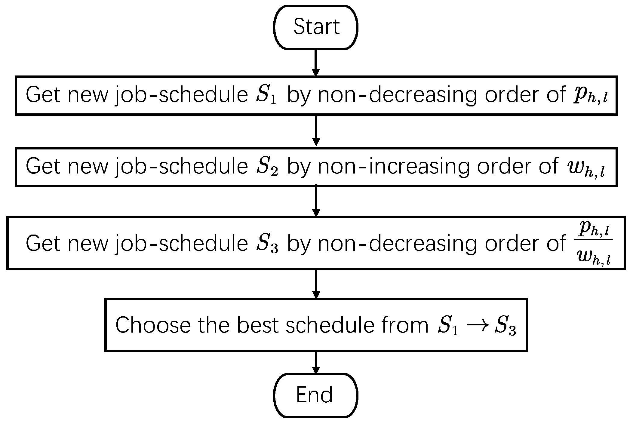
| Algorithm 1 for of minimizing |
| Step (1). Jobs in are arranged by the non-decreasing order of . Step (2). Jobs in are arranged by the non-increasing order of . Step (3). Jobs in are arranged by the non-decreasing order of . Step (4). Choose the better solution from Steps (1)–(3). |
4.2. Group Schedule
| Algorithm 2 for group schedule |
| Step (1). Groups are arranged by the non-decreasing (non-increasing) order of , Step (2). Groups are arranged by the non-decreasing (non-increasing) order of , Step (3). Groups are arranged by the non-decreasing (non-increasing) order of , Step (4). Groups are arranged by the non-decreasing (non-increasing) order of , Step (5). Groups are arranged by the non-decreasing (non-increasing) order of , Step (6). Groups are arranged by the non-decreasing (non-increasing) order of , Step (7). Groups are arranged by the non-decreasing (non-increasing) order of , Step (8). Groups are arranged by the non-decreasing (non-increasing) order of , Step (9). Groups are arranged by the non-decreasing (non-increasing) order of , Step (10). Choose the one with smaller value as the solution by Steps (1)–(9). |
4.3. Solution Algorithms
| Algorithm 3 algorithm |
| Step (1). For each group , the optimal job schedule is obtained by the algorithm, where the lower bound is Equation (8) (see Theorem 4) and the upper bound is calculated by Algorithm 1, and . Step (2). The optimal group schedule is obtained by the algorithm, where the lower bound is Equation (11) (see Theorem 5) and the upper bound is calculated by Algorithm 2. |
| Algorithm 4 algorithm |
| Step (1-1). For group , let be a job schedule obtained from Algorithm 1, . Step (1-2). Set . Select the first two jobs from the sorted list and select the better of the two possible job schedules. Do not change the relative positions of these two jobs with respect to each other in the remaining steps of the algorithm. Set . Step (1-3). Pick the job in the th position of the list generated in Step (1-1) and find the best job schedule by placing it at all possible positions in the partial schedule found in the previous step, without changing the relative positions to each other of the already assigned jobs. Step (1-4). If , STOP; otherwise, set and go to Step (1-3). Step (2-1). Let be a group schedule obtained from Algorithm 2. Step (2-2). Set . Select the first two groups from the sorted list and select the better of the two possible group schedules. Do not change the relative positions of these two groups with respect to each other in the remaining steps of the algorithm. Set . Step (2-3). Pick the group in the th position of the list generated in Step (2-1) and find the best group schedule by placing it at all possible positions in the partial group schedule found in the previous step, without changing the relative positions to each other of the already assigned groups. Step (2-4). If , STOP; otherwise, set and go to Step (2-3). |
| Algorithm 5 algorithm |
| Step (1-1). For group , let be a job schedule obtained from Algorithm 1, . Step (1-2). Calculate the cost value of the original job schedule for (see Equation (7)). Step (1-3). Calculate the cost value of the new job schedule by using the pairwise interchange (PI) neighborhood method. If is less than , it is accepted. Nevertheless, if is higher, it might still be accepted with a decreasing probability as the process proceeds. This acceptance probability is determined by the following exponential distribution function: where is a parameter and is the change in the objective cost . In addition, the method is used to change in the kth iteration as follows: where is a constant. After preliminary trials, is used. Step (1-4). If increases, the new job schedule is accepted when , where is randomly sampled from the uniform distribution. Step (1-5). The job schedule is stable after iterations. Step (2-1). Let be a group schedule obtained from Algorithm 2. Step (2-2). Calculate the cost value of the original group schedule (see Equation (10)). Step (2-3). Calculate the cost value of the new group schedule by using the PI neighborhood method. If is less than , it is accepted. Nevertheless, if is higher, it might still be accepted with a decreasing probability as the process proceeds. This acceptance probability is determined by the following exponential distribution function: where is a parameter and is the change in the objective cost . In addition, the method is used to change in the kth iteration as follows: where is a constant. After preliminary trials, is used. Step (2-4). If increases, the new group schedule is accepted when , where is randomly sampled from the uniform distribution. Step (2-5). The group schedule is stable after iterations. |
5. Experimental Study
6. Conclusions
Author Contributions
Funding
Data Availability Statement
Conflicts of Interest
References
- Xue, Y.; Rui, Z.J.; Yu, X.Y.; Sang, X.Z.; Liu, W.J. Estimation of distribution evolution memetic algorithm for the unrelated parallel-machine green scheduling problem. Memetic Comput. 2019, 11, 423–437. [Google Scholar] [CrossRef]
- Foumani, M.; Smith-Miles, K. The impact of various carbon reduction policies on green flowshop scheduling. Appl. Energy 2019, 249, 300–315. [Google Scholar] [CrossRef]
- Li, M.; Wang, G.G. A review of green shop scheduling problem. Inf. Sci. 2022, 589, 478–496. [Google Scholar] [CrossRef]
- Kong, F.Y.; Song, J.X.; Miao, C.X.; Zhang, Y.Z. Scheduling problems with rejection in green manufacturing industry. J. Comb. Optim. 2025, 49, 63. [Google Scholar] [CrossRef]
- Yin, Y.; Wu, W.-H.; Cheng, T.C.E.; Wu, C.-C. Single-machine scheduling with time-dependent and position-dependent deteriorating jobs. Int. J. Comput. Integr. Manuf. 2015, 28, 781–790. [Google Scholar] [CrossRef]
- Huang, X.; Wang, J.-J. Machine scheduling problems with a position-dependent deterioration. Appl. Math. Model. 2015, 39, 2897–2908. [Google Scholar] [CrossRef]
- Pei, J.; Wang, X.; Fan, W.; Pardalos, P.M.; Liu, X. Scheduling step-deteriorating jobs on bounded parallel-batching machines to maximise the total net revenue. J. Oper. Res. Soc. 2019, 70, 1830–1847. [Google Scholar] [CrossRef]
- Gawiejnowicz, S. Models and Algorithms of Time-Dependent Scheduling; Springer: Berlin/Heidelberg, Germany, 2020. [Google Scholar]
- Lu, Y.-Y.; Teng, F.; Feng, Z.-X. Scheduling jobs with truncated exponential sum-of-logarithm-processing-times based and position-based learning effects. Asia-Pac. J. Oper. Res. 2015, 32, 1550026. [Google Scholar] [CrossRef]
- Jiang, Z.; Chen, F.; Zhang, X. Single-machine scheduling with times-based and job-dependent learning effect. J. Oper. Res. Soc. 2017, 68, 809–815. [Google Scholar] [CrossRef]
- Azzouz, A.; Ennigrou, M.; Ben Said, L. Scheduling problems under learning effects: Classification and cartography. Int. J. Prod. Res. 2018, 56, 1642–1661. [Google Scholar] [CrossRef]
- Sun, X.Y.; Geng, X.-N.; Liu, F. Flow shop scheduling with general position weighted learning effects to minimise total weighted completion time. J. Oper. Res. Soc. 2021, 72, 2674–2689. [Google Scholar] [CrossRef]
- Wang, J.-B.; Lv, D.-Y.; Xu, J.; Ji, P.; Li, F. Bicriterion scheduling with truncated learning effects and convex controllable processing times. Int. Trans. Oper. Res. 2021, 28, 1573–1593. [Google Scholar] [CrossRef]
- Pei, J.; Zhou, Y.; Yan, P.; Pardalos, P.M. A concise guide to scheduling with learning and deteriorating effects. Int. J. Prod. Res. 2021, 61, 2010–2031. [Google Scholar] [CrossRef]
- Keshavarz, T.; Savelsbergh, M.; Salmasi, N. A branch-and-bound algorithm for the single machine sequence-dependent group scheduling problem with earliness and tardiness penalties. Appl. Math. Model. 2015, 39, 6410–6424. [Google Scholar] [CrossRef]
- Ji, M.; Zhang, X.; Tang, X.Y.; Cheng, T.C.E.; Wei, G.Y.; Tan, Y.Y. Group scheduling with group-dependent multiple due-windows assignment. Int. J. Prod. Res. 2016, 54, 1244–1256. [Google Scholar] [CrossRef]
- Neufeld, J.S.; Gupta, J.N.D.; Buscher, U. A comprehensive review of flowshop group scheduling literature. Comput. Oper. Res. 2016, 70, 56–74. [Google Scholar] [CrossRef]
- Wang, J.-B.; Liang, X.-X. Group scheduling with deteriorating jobs and allotted resource under limited resource availability constraint. Eng. Optim. 2019, 51, 231–246. [Google Scholar] [CrossRef]
- Ning, L.; Sun, L. Single-machine group scheduling problems with general deterioration and linear learning effects. Math. Probl. Eng. 2023, 2023, 1455274. [Google Scholar] [CrossRef]
- Zhao, S. Scheduling jobs with general truncated learning effects including proportional setup times. Comput. Appl. Math. 2022, 41, 146. [Google Scholar] [CrossRef]
- Wu, C.-C.; Lin, W.-C.; Azzouz, A.; Xu, J.Y.; Chiu, Y.-L.; Tsai, Y.-W.; Shen, P.Y. A bicriterion single-machine scheduling problem with step-improving processing times. Comput. Ind. Eng. 2022, 171, 108469. [Google Scholar] [CrossRef]
- Ma, R.; Guo, S.A.; Zhang, X.Y. An optimal online algorithm for single-processor scheduling problem with learning effect. Theor. Comput. Sci. 2023, 928, 1–12. [Google Scholar] [CrossRef]
- Miao, C.; Song, J.; Zhang, Y. Single-machine time-dependent scheduling with proportional and delivery times. Asia-Pac. J. Oper. Res. 2023, 40, 2240015. [Google Scholar] [CrossRef]
- Lu, Y.-Y.; Zhang, S.; Tao, J.-Y. Earliness–tardiness scheduling with delivery times and deteriorating jobs. Asia-Pac. J. Oper. Res. 2025, 42, 2450009. [Google Scholar] [CrossRef]
- Sun, X.Y.; Liu, T.; Geng, X.-N.; Hu, Y.; Xu, J.-X. Optimization of scheduling problems with deterioration effects and an optional maintenance activity. J. Sched. 2023, 26, 251–266. [Google Scholar] [CrossRef]
- Zhang, L.-H.; Lv, D.-Y.; Wang, J.-B. Two-agent slack due-date assignment scheduling with resource allocations and deteriorating jobs. Mathematics 2023, 11, 2737. [Google Scholar] [CrossRef]
- Zhang, L.-H.; Geng, X.-N.; Xue, J.; Wang, J.-B. Single machine slack due-window assignment and deteriorating jobs. J. Ind. Manag. 2024, 20, 1593–1614. [Google Scholar] [CrossRef]
- Liu, Z.; Wang, J.-B. Single-machine scheduling with simultaneous learning effects and delivery times. Mathematics 2024, 12, 2522. [Google Scholar] [CrossRef]
- Wang, J.-B.; Wang, Y.-C.; Wan, C.; Lv, D.-Y.; Zhang, L. Controllable processing time scheduling with total weighted completion time objective and deteriorating jobs. Asia-Pac. J. Oper. Res. 2024, 41, 2350026. [Google Scholar] [CrossRef]
- Lv, Z.-G.; Zhang, L.-H.; Wang, X.-Y.; Wang, J.-B. Single machine scheduling proportionally deteriorating jobs with ready times subject to the total weighted completion time minimization. Mathematics 2024, 12, 610. [Google Scholar] [CrossRef]
- Qian, J.; Chang, G.; Zhang, X. Single-machine common due-window assignment and scheduling with position-dependent weights, delivery time, learning effect and resource allocations. J. Appl. Math. Comput. 2024, 70, 1965–1994. [Google Scholar] [CrossRef]
- Qian, J.; Guo, Z.-Y. Common due-window assignment and single machine scheduling with delivery time, resource allocation, and job-dependent learning effect. J. Appl. Math. Comput. 2024, 70, 4441–4471. [Google Scholar] [CrossRef]
- Mao, R.-R.; Lv, D.-Y.; Ren, N.; Wang, J.-B. Supply chain scheduling with deteriorating jobs and delivery times. J. Appl. Math. Comput. 2024, 70, 2285–2312. [Google Scholar] [CrossRef]
- Lv, D.-Y.; Xue, J.; Wang, J.-B. Minmax common due-window assignment scheduling with deteriorating jobs. J. Oper. Res. Soc. China 2024, 12, 681–693. [Google Scholar] [CrossRef]
- Qiu, X.-Y.; Wang, J.-B. Single-machine scheduling with mixed due-windows and deterioration effects. J. Appl. Math. Comput. 2025, 71, 2527–2542. [Google Scholar] [CrossRef]
- Lv, D.-Y.; Wang, J.-B. No-idle flow shop scheduling with deteriorating jobs and common due date under dominating machines. Asia-Pac. J. Oper. Res. 2024, 41, 2450003. [Google Scholar] [CrossRef]
- Paredes-Astudillo, Y.A.; Botta-Genoulaz, V.; Montoya-Torres, J.R. Impact of learning effect modelling in flowshop scheduling with makespan minimisation based on the Nawaz–Enscore–Ham algorithm. Int. J. Prod. Res. 2024, 62, 1999–2014. [Google Scholar] [CrossRef]
- Parichehreh, M.; Gholizadeh, H.; Fathollahi-Fard, A.M.; Wong, K.Y. An energy-efficient unrelated parallel machine scheduling problem with learning effect of operators and deterioration of jobs. Int. J. Environ. Sci. Technol. 2024, 21, 9651–9676. [Google Scholar] [CrossRef]
- Bai, B.; Wei, C.-M.; He, H.-Y.; Wang, J.-B. Study on single-machine common/slack due-window assignment scheduling with delivery times, variable processing times and outsourcing. Mathematics 2024, 12, 2833. [Google Scholar] [CrossRef]
- Lv, D.-Y.; Wang, J.-B. Considering the peak power consumption problem with learning and deterioration effect in flow shop scheduling. Comput. Ind. Eng. 2024, 197, 110599. [Google Scholar] [CrossRef]
- Lv, D.-Y.; Wang, J.-B. Research on two-machine flow shop scheduling problem with release dates and truncated learning effects. Eng. Optim. 2024. [Google Scholar] [CrossRef]
- Wang, X.-Y.; Lv, D.-Y.; Ji, P.; Yin, N.; Wang, J.-B.; Jin, Q. Single machine scheduling problems with truncated learning effects and exponential past-sequence-dependent delivery times. Comput. Appl. Math. 2024, 43, 194. [Google Scholar] [CrossRef]
- Zhang, Y.Y.; Sun, X.-Y.; Liu, T.; Wang, J.Y.; Geng, X.-N. Single-machine scheduling simultaneous consideration of resource allocations and exponential time-dependent learning effects. J. Oper. Res. Soc. 2025, 76, 528–540. [Google Scholar] [CrossRef]
- Zhang, L.-H.; Yang, S.-H.; Lv, D.-Y.; Wang, J.-B. Research on convex resource allocation scheduling with exponential time-dependent learning effects. Comput. J. 2025, 68, 97–108. [Google Scholar] [CrossRef]
- Song, J.X.; Miao, C.X.; Kong, F.Y. Scheduling with step learning and job rejection. Oper. Res. 2025, 25, 6. [Google Scholar] [CrossRef]
- Sun, Z.-W.; Lv, D.-Y.; Wei, C.-M.; Wang, J.-B. Flow shop scheduling with shortening jobs for makespan minimization. Mathematics 2025, 13, 363. [Google Scholar] [CrossRef]
- Wang, X.Y.; Liu, W.G. Delivery scheduling with variable processing times and due date assignments. Bull. Malays. Math. Sci. Soc. 2025, 48, 76. [Google Scholar] [CrossRef]
- Sun, Y.; He, H.; Zhao, Y.; Wang, J.-B. Minimizing makespan scheduling on a single machine with general positional deterioration effects. Axioms 2025, 14, 290. [Google Scholar] [CrossRef]
- Sun, Y.; Lv, D.-Y.; Huang, X. Properties for due-window assignment scheduling on a two-machine no-wait proportionate flow shop with learning effects and resource allocation. J. Oper. Res. Soc. 2025. [Google Scholar] [CrossRef]
- Kuo, W.-H.; Yang, D.-L. Single-machine group scheduling with a time-dependent learning effect. Comput. Oper. Res. 2006, 33, 2099–2112. [Google Scholar] [CrossRef]
- Wu, C.-C.; Lee, W.-C. Single-machine group-scheduling problems with deteriorating setup times and job-processing times. Int. Prod. Econ. 2008, 115, 128–133. [Google Scholar] [CrossRef]
- Lee, W.-C.; Wu, C.-C. A note on single-machine group scheduling problems with position-based learning effect. Appl. Math. Model. 2009, 33, 2159–2163. [Google Scholar] [CrossRef]
- Yang, S.-J.; Yang, D.-L. Single-machine group scheduling problems under the effects of deterioration and learning. Comput. Ind. Eng. 2010, 58, 754–758. [Google Scholar] [CrossRef]
- Kuo, W.-H. Single-machine group scheduling with time-dependent learning effect and position-based setup time learning effect. Ann. Oper. Res. 2012, 196, 349–359. [Google Scholar] [CrossRef]
- He, Y.; Sun, L. One-machine scheduling problems with deteriorating jobs and position-dependent learning effects under group technology considerations. Int. J. Syst. Sci. 2015, 46, 1319–1326. [Google Scholar] [CrossRef]
- Fan, W.; Pei, J.; Liu, X.; Pardalos, P.M.; Kong, M. Serial-batching group scheduling with release times and the combined effects of deterioration and truncated job-dependent learning. J. Glob. Optim. 2018, 71, 147–163. [Google Scholar] [CrossRef]
- Huang, X. Bicriterion scheduling with group technology and deterioration effect. J. Appl. Math. Comput. 2019, 60, 455–464. [Google Scholar] [CrossRef]
- Liu, F.; Yang, J.; Lu, Y.-Y. Solution algorithms for single-machine group scheduling with ready times and deteriorating jobs. Eng. Optim. 2019, 51, 862–874. [Google Scholar] [CrossRef]
- Miao, C.X. Parallel-batch scheduling with deterioration and group technology. IEEE Access 2019, 7, 119082–119086. [Google Scholar] [CrossRef]
- Sun, L.; Ning, L.; Huo, J.-Z. Group scheduling problems with time-dependent and position-dependent DeJong’s learning effect. Math. Probl. Eng. 2020, 2020, 5161872. [Google Scholar] [CrossRef]
- Xu, H.; Li, X.; Ruiz, R.; Zhu, H. Group scheduling with nonperiodical maintenance and deteriorating effects. IEEE Trans. Syst. Man-Cybern.-Syst. 2021, 51, 2860–2872. [Google Scholar] [CrossRef]
- Liu, S.-C. Common due-window assignment and group scheduling with position-dependent processing times. Asia-Pac. J. Oper. Res. 2023, 32, 1550045. [Google Scholar] [CrossRef]
- Yan, J.-X.; Ren, N.; Bei, H.-B.; Bao, H.; Wang, J.-B. Study on resource allocation scheduling problem with learning factors and group technology. J. Ind. Manag. Optim. 2023, 19, 3419–3435. [Google Scholar] [CrossRef]
- Liu, W.G.; Wang, X.Y. Group technology scheduling with due-date assignment and controllable processing times. Processes 2023, 11, 1271. [Google Scholar] [CrossRef]
- Chen, K.; Han, S.; Huang, H.; Ji, M. A group-dependent due-window assignment scheduling problem with controllable learning effect. Asia-Pac. J. Oper. Res. 2023, 40, 2250025. [Google Scholar] [CrossRef]
- Li, M.-H.; Lv, D.-Y.; Lu, Y.-Y.; Wang, J.-B. Scheduling with group technology, resource allocation, and learning effect simultaneously. Mathematics 2024, 12, 1029. [Google Scholar] [CrossRef]
- Li, M.-H.; Lv, D.-Y.; Lv, Z.-G.; Zhang, L.-H.; Wang, J.-B. A two-agent resource allocation scheduling problem with slack due-date assignment and general deterioration function. Comput. Appl. Math. 2024, 43, 229. [Google Scholar] [CrossRef]
- Lv, D.-Y.; Wang, J.-B. Single-machine group technology scheduling with resource allocation and slack due-window assignment including minmax criterion. J. Oper. Res. Soc. 2024. [Google Scholar] [CrossRef]
- Wang, X.Y.; Liu, W.G. Optimal different due-dates assignment scheduling with group technology and resource allocation. Mathematics 2024, 12, 436. [Google Scholar] [CrossRef]
- Wang, X.Y.; Liu, W.G. Single machine group scheduling jobs with resource allocations subject to unrestricted due date assignments. J. Appl. Math. Comput. 2024, 70, 6283–6308. [Google Scholar] [CrossRef]
- Yin, N.; Gao, M. Single-machine group scheduling with general linear deterioration and truncated learning effects. Comput. Appl. Math. 2024, 43, 386. [Google Scholar] [CrossRef]
- Zhang, Z.Q.; Xu, Y.X.; Qian, B.; Hu, R.; Wu, F.C.; Wang, L. An enhanced estimation of distribution algorithm with problem-specific knowledge for distributed no-wait flowshop group scheduling problems. Swarm Evol. Comput. 2024, 87, 101559. [Google Scholar] [CrossRef]
- Wang, B.T.; Pan, Q.K.; Gao, L.; Li, W.M. The paradoxes, accelerations and heuristics for a constrained distributed flowshop group scheduling problem. Comput. Ind. Eng. 2024, 196, 110465. [Google Scholar] [CrossRef]
- Han, Z.D.; Zhang, B.; Sang, H.Y.; Lu, C.; Meng, L.L.; Zou, W.Q. Optimising distributed heterogeneous flowshop group scheduling arising from PCB mounting: Integrating construction and improvement heuristics. Int. J. Prod. Res. 2025, 63, 1753–1778. [Google Scholar] [CrossRef]
- Li, M.; Goossens, D. Grouping and scheduling multiple sports leagues: An integrated approach. J. Oper. Res. Soc. 2025, 76, 739–757. [Google Scholar] [CrossRef]
- Miao, J.-D.; Lv, D.-Y.; Wei, C.-M.; Wang, J.-B. Research on group scheduling with general logarithmic deterioration subject to maximal completion time cost. Axioms 2025, 14, 153. [Google Scholar] [CrossRef]
- Browne, S.; Yechiali, U. Scheduling deteriorating jobs on a single processor. Oper. Res. 1990, 38, 495–498. [Google Scholar] [CrossRef]
- Bachman, A.; Janiak, A.; Kovalyov, M.Y. Minimizing the total weighted completion time of deteriorating jobs. Inf. Process. Lett. 2002, 81, 81–84. [Google Scholar] [CrossRef]
- Nawaz, M.; Enscore, E.E.; Ham, I. A heuristic algorithm for the m-machine, n-job flow-shop sequencing problem. Omega 1983, 11, 91–95. [Google Scholar] [CrossRef]
- Li, M.-H.; Lv, D.-Y.; Zhang, L.-H.; Wang, J.-B. Permutation flow shop scheduling with makespan objective and truncated learning effects. J. Appl. Math. Comput. 2024, 70, 2907–2939. [Google Scholar] [CrossRef]
- Mor, B.; Shapira, D. Single machine scheduling with non-availability interval and optional job rejection. J. Comb. Optim. 2022, 44, 480–497. [Google Scholar] [CrossRef]
- Geng, X.-N.; Sun, X.; Wang, J.-Y.; Pan, L. Scheduling on proportionate flow shop with job rejection and common due date assignment. Comput. Ind. Eng. 2023, 181, 109317. [Google Scholar] [CrossRef]
- Chen, R.-X.; Li, S.-S. Two-machine job shop scheduling with optional job rejection. Optim. Lett. 2024, 18, 1593–1618. [Google Scholar] [CrossRef]
- Wang, J.-B.; Bao, H.; Wan, C. Research on multiple slack due-date assignments scheduling with position-dependent weights. Asia-Pac. J. Oper. Res. 2024, 41, 2350039. [Google Scholar] [CrossRef]
- Wang, J.-B.; Lv, D.-Y.; Wan, C. Proportionate flow shop scheduling with job-dependent due-windows and position-dependent weights. Asia-Pac. J. Oper. Res. 2025, 42, 2450011. [Google Scholar] [CrossRef]
- Wang, J.-J.; Wang, L. Decoding methods for the flow shop scheduling with peak power consumption constraints. Int. J. Prod. Res. 2019, 57, 3200–3218. [Google Scholar] [CrossRef]
- Arani, M.; Momenitabar, M.; Priyanka, T.J. Unrelated parallel machine scheduling problem considering job splitting, inventories, shortage, and resource: A meta-heuristic approach. Systems 2024, 12, 37. [Google Scholar] [CrossRef]


| Reference | Objective Function | Setup Time | Job-Processing Time | Solution Method |
|---|---|---|---|---|
| Kuo and Yang [50] | Makespan | constant number | , | Polynomial time algorithm |
| Total completion time | constant number | , | Heuristic algorithm | |
| Wu et al. [51] | Makespan | , | , | Polynomial time algorithm |
| Total completion time | , | , | Heuristic algorithm | |
| Lee and Wu [52] | Makespan | Polynomial time algorithm | ||
| Total completion time | Polynomial time algorithm | |||
| under a special condition | ||||
| Yang and Yang [53] | Makespan | , | , | Polynomial time algorithm |
| Makespan | , | , | Polynomial time algorithm | |
| Total completion time | , | , | Polynomial time algorithm | |
| under a special condition | ||||
| Total completion time | , | , | Polynomial time algorithm | |
| under a special condition | ||||
| Kuo [54] | Makespan | , | , | Polynomial time algorithm |
| Total completion time | , | , | Heuristic algorithm | |
| He and Sun [55] | Makespan, | , | -, | Polynomial time algorithm |
| Total completion time | , | -, | Polynomial time algorithm | |
| under a special condition | ||||
| Fan et al. [56] | Makespan | , , | -, | Heuristic algorithm |
| Huang [57] | Maximum cost on the set of | , | , | Polynomial time algorithm |
| minimizing total weighted completion time | ||||
| Liu et al. [58] | Makespan | constant number | , | Heuristic algorithm, |
| branch-and-bound algorithm | ||||
| Sun et al. [60] | Makespan | constant number | , | Polynomial time algorithm |
| Total completion time | constant number | , | Polynomial time algorithm | |
| Total weighted completion time | constant number | , | Polynomial time algorithm | |
| under a special condition | ||||
| Liu [62] | Earliness–tardiness cost | constant number | , | Polynomial time algorithm |
| Miao et al. [76] | Makespan | Polynomial time algorithm | ||
| Ning and Sun [19] | Makespan | , | , | Polynomial time algorithm |
| total (weighted) completion time | , | , | Polynomial time algorithm | |
| under a special condition | ||||
| This paper | total weighted completion time | , | , | Heuristic algorithm, |
| simulated annealing, | ||||
| branch-and-bound algorithm |
| min | avg | max | min | avg | max | min | avg | max | ||
| 263.1 | 354.5 | 467.9 | 402.5 | 432.6 | 476.0 | 3808.7 | 19,792.0 | 75,060.7 | ||
| 60 × 11 | 283.8 | 392.7 | 473.5 | 400.9 | 431.7 | 461.4 | 375.0 | 1530.7 | 3866.2 | |
| 277.4 | 388.3 | 471.6 | 404.7 | 436.1 | 472.0 | 175.5 | 610.5 | 1434.9 | ||
| 312.4 | 390.5 | 483.2 | 413.9 | 450.2 | 480.9 | 7215.5 | 69,538.0 | 279,511.2 | ||
| 60 × 12 | 233.5 | 393.9 | 502.6 | 400.1 | 444.4 | 484.7 | 509.7 | 2433.8 | 6264.7 | |
| 265.5 | 408.1 | 506.4 | 418.1 | 448.6 | 499.6 | 163.0 | 1037.4 | 3886.2 | ||
| 215.5 | 401.8 | 485.5 | 438.4 | 467.9 | 507.7 | 15,793.4 | 179,221.5 | 697,682.1 | ||
| 60 × 13 | 279.1 | 399.7 | 502.1 | 436.4 | 469.4 | 521.6 | 1574.3 | 4878.0 | 14410.0 | |
| 303.4 | 405.0 | 529.6 | 444.1 | 472.4 | 514.9 | 414.2 | 1878.3 | 5713.7 | ||
| 267.4 | 390.9 | 464.0 | 424.6 | 450.7 | 516.0 | 54,801.6 | 549,690.8 | 2,392,813.2 | ||
| 60 × 14 | 277.2 | 376.7 | 459.7 | 423.7 | 430.8 | 438.1 | 1524.3 | 7593.3 | 19,410.4 | |
| 269.0 | 364.8 | 469.3 | 425.8 | 441.7 | 492.6 | 647.2 | 4013.9 | 15,599.9 | ||
| 406.7 | 558.0 | 716.6 | 626.4 | 669.3 | 716.1 | 3921.6 | 31,745.4 | 68,998.1 | ||
| 80 × 11 | 467.0 | 612.6 | 726.7 | 639.5 | 669.0 | 720.1 | 1073.1 | 1869.4 | 3650.2 | |
| 417.7 | 593.1 | 713.9 | 628.3 | 676.3 | 757.4 | 750.2 | 1316.5 | 2027.9 | ||
| 367.8 | 564.5 | 730.9 | 621.5 | 664.7 | 726.8 | 18,034.9 | 121,560.8 | 546,209.1 | ||
| 80 × 12 | 384.6 | 567.4 | 722.2 | 622.2 | 666.6 | 736.5 | 1106.9 | 3602.7 | 8693.4 | |
| 379.5 | 573.5 | 727.8 | 627.1 | 658.5 | 722.7 | 412.5 | 1606.4 | 4862.8 | ||
| 467.6 | 614.7 | 750.3 | 655.3 | 708.6 | 773.1 | 47,222.5 | 399,686.6 | 1,426,509.1 | ||
| 80 × 13 | 486.0 | 605.3 | 744.7 | 670.7 | 719.3 | 770.0 | 1244.3 | 4917.5 | 13,859.8 | |
| 461.7 | 618.4 | 765.9 | 656.8 | 700.0 | 747.4 | 863.6 | 3547.1 | 10708.3 | ||
| 430.5 | 573.1 | 732.7 | 636.0 | 657.3 | 740.8 | 47,602.9 | 1,014,303.5 | 2,944,199.4 | ||
| 80 × 14 | 411.6 | 603.9 | 810.5 | 673.3 | 696.6 | 759.3 | 1741.8 | 12,841.9 | 46,554.5 | |
| 395.4 | 603.2 | 788.1 | 691.0 | 737.9 | 876.2 | 1002.0 | 5147.7 | 16,667.3 | ||
| 643.5 | 962.3 | 1251.2 | 1066.4 | 1123.9 | 1187.1 | 24,913.5 | 60,882.7 | 186,142.1 | ||
| 100 × 11 | 817.8 | 1020.0 | 1254.9 | 1074.3 | 1138.7 | 1189.4 | 6061.0 | 10,114.1 | 16,456.4 | |
| 697.3 | 943.4 | 1260.7 | 1067.7 | 1137.0 | 1225.0 | 4190.2 | 9763.6 | 17,136.9 | ||
| 669.6 | 924.2 | 1193.1 | 1042.3 | 1109.9 | 1154.6 | 43,013.2 | 161,464.9 | 459,263.5 | ||
| 100 × 12 | 575.1 | 917.4 | 1219.4 | 1047.8 | 1115.1 | 1164.5 | 3508.0 | 8094.9 | 14,471.8 | |
| 667.5 | 942.5 | 1150.9 | 1030.9 | 1112.7 | 1167.6 | 2581.2 | 5016.4 | 8090.7 | ||
| 720.5 | 895.3 | 1165.7 | 956.2 | 1055.4 | 1208.1 | 92,587.4 | 442,220.3 | 1,246,050.5 | ||
| 100 × 13 | 641.7 | 889.0 | 1090.0 | 976.2 | 1027.1 | 1085.2 | 2657.0 | 10,081.4 | 29,144.3 | |
| 538.0 | 828.2 | 1100.5 | 1001.6 | 1035.3 | 1086.1 | 2207.5 | 4644.5 | 7919.2 | ||
| 473.3 | 854.7 | 1117.6 | 942.3 | 1035.7 | 1142.3 | 144,583.6 | 1,498,611.1 | 9,996,035.7 | ||
| 100 × 14 | 598.7 | 837.7 | 1113.2 | 975.3 | 1047.7 | 1094.6 | 3755.3 | 16,910.9 | 43,546.8 | |
| 658.5 | 925.2 | 1188.1 | 1010.9 | 1067.8 | 1158.7 | 2499.8 | 8020.0 | 26,848.7 | ||
| min | avg | max | min | avg | max | ||
| 1.0000 | 1.0127 | 1.0721 | 1.0000 | 1.0036 | 1.0316 | ||
| 60 × 11 | 1.0000 | 1.0160 | 1.1950 | 1.0000 | 1.0047 | 1.0551 | |
| 1.0000 | 1.0074 | 1.0829 | 1.0000 | 1.0068 | 1.0829 | ||
| 1.0000 | 1.0170 | 1.1045 | 1.0000 | 1.0029 | 1.0287 | ||
| 60 × 12 | 1.0000 | 1.0126 | 1.0984 | 1.0000 | 1.0063 | 1.0936 | |
| 1.0000 | 1.0093 | 1.1142 | 1.0000 | 1.0018 | 1.0261 | ||
| 1.0000 | 1.0036 | 1.0237 | 1.0000 | 1.0020 | 1.0252 | ||
| 60 × 13 | 1.0000 | 1.0167 | 1.1618 | 1.0000 | 1.0021 | 1.0249 | |
| 1.0000 | 1.0067 | 1.0593 | 1.0000 | 1.0009 | 1.0128 | ||
| 1.0000 | 1.0093 | 1.0723 | 1.0000 | 1.0042 | 1.0464 | ||
| 60 × 14 | 1.0000 | 1.0026 | 1.0221 | 1.0000 | 1.0024 | 1.0678 | |
| 1.0000 | 1.0085 | 1.2122 | 1.0000 | 1.0080 | 1.2121 | ||
| 1.0000 | 1.0138 | 1.0765 | 1.0000 | 1.0031 | 1.0563 | ||
| 80 × 11 | 1.0000 | 1.0031 | 1.0305 | 1.0000 | 1.0066 | 1.0817 | |
| 1.0000 | 1.0074 | 1.0818 | 1.0000 | 1.0024 | 1.0578 | ||
| 1.0000 | 1.0097 | 1.0772 | 1.0000 | 1.0024 | 1.0299 | ||
| 80 × 12 | 1.0000 | 1.0110 | 1.1240 | 1.0000 | 1.0035 | 1.0359 | |
| 1.0000 | 1.0114 | 1.1427 | 1.0000 | 1.0006 | 1.0124 | ||
| 1.0000 | 1.0133 | 1.0766 | 1.0000 | 1.0021 | 1.0223 | ||
| 80 × 13 | 1.0000 | 1.0026 | 1.0581 | 1.0000 | 1.0014 | 1.0109 | |
| 1.0000 | 1.0261 | 1.1826 | 1.0000 | 1.0172 | 1.1826 | ||
| 1.0000 | 1.0127 | 1.0832 | 1.0000 | 1.0067 | 1.1386 | ||
| 80 × 14 | 1.0000 | 1.0050 | 1.0281 | 1.0000 | 1.0028 | 1.0247 | |
| 1.0000 | 1.0185 | 1.1001 | 1.0000 | 1.0112 | 1.1001 | ||
| 1.0000 | 1.0200 | 1.0757 | 1.0000 | 1.0055 | 1.0491 | ||
| 100 × 11 | 1.0000 | 1.0062 | 1.1459 | 1.0000 | 1.0048 | 1.0456 | |
| 1.0000 | 1.0027 | 1.0387 | 1.0000 | 1.0020 | 1.0230 | ||
| 1.0000 | 1.0160 | 1.1511 | 1.0000 | 1.0081 | 1.1511 | ||
| 100 × 12 | 1.0000 | 1.0086 | 1.2021 | 1.0000 | 1.0028 | 1.0509 | |
| 1.0000 | 1.0243 | 1.2419 | 1.0000 | 1.0169 | 1.1877 | ||
| 1.0000 | 1.0091 | 1.0498 | 1.0000 | 1.0047 | 1.0588 | ||
| 100 × 13 | 1.0000 | 1.0029 | 1.0378 | 1.0000 | 1.0022 | 1.0192 | |
| 1.0000 | 1.0040 | 1.0420 | 1.0000 | 1.0037 | 1.0648 | ||
| 1.0000 | 1.0096 | 1.0524 | 1.0000 | 1.0030 | 1.0210 | ||
| 100 × 14 | 1.0000 | 1.0053 | 1.1138 | 1.0000 | 1.0012 | 1.0100 | |
| 1.0000 | 1.0067 | 1.1480 | 1.0000 | 1.0003 | 1.0044 | ||
| min | avg | max | min | avg | max | min | avg | max | ||
| 269.6 | 397.9 | 488.5 | 416.2 | 445.3 | 499.5 | 8885.6 | 33,664.2 | 96,546.1 | ||
| 60 × 11 | 282.9 | 396.4 | 484.0 | 423.6 | 446.2 | 478.6 | 759.4 | 2835.2 | 6168.7 | |
| 312.6 | 394.5 | 490.7 | 424.4 | 449.2 | 485.7 | 337.5 | 1024.9 | 2329.0 | ||
| 267.9 | 381.9 | 468.1 | 419.7 | 445.9 | 485.5 | 57,453.6 | 203,469.6 | 843,915.7 | ||
| 60 × 12 | 275.3 | 376.0 | 456.9 | 414.7 | 444.4 | 471.2 | 2961.5 | 5430.9 | 10,209.0 | |
| 206.3 | 374.9 | 478.1 | 412.7 | 435.9 | 481.1 | 613.7 | 1856.5 | 5276.0 | ||
| 276.0 | 378.2 | 494.4 | 415.4 | 443.2 | 492.9 | 109,707.8 | 458,420.7 | 1,258,305.9 | ||
| 60 × 13 | 286.6 | 368.8 | 480.4 | 408.7 | 436.6 | 487.6 | 2424.6 | 8797.8 | 26,448.4 | |
| 269.0 | 375.4 | 481.2 | 409.2 | 438.2 | 498.9 | 380.2 | 3259.4 | 8612.4 | ||
| 277.8 | 379.8 | 479.8 | 416.9 | 460.4 | 541.5 | 146,566.9 | 1,546,453.4 | 6,929,877.7 | ||
| 60 × 14 | 280.1 | 385.4 | 493.5 | 433.8 | 455.9 | 506.4 | 8227.7 | 25,103.3 | 47,670.7 | |
| 244.3 | 370.9 | 496.7 | 429.5 | 454.2 | 513.7 | 1507.8 | 7019.6 | 19,387.9 | ||
| 414.4 | 575.3 | 722.1 | 625.8 | 667.5 | 720.8 | 21,585.3 | 56,004.2 | 126,105.0 | ||
| 80 × 11 | 442.2 | 613.5 | 735.3 | 658.8 | 686.3 | 723.4 | 2837.4 | 4985.4 | 9074.5 | |
| 455.5 | 605.5 | 724.7 | 655.9 | 677.7 | 716.1 | 1973.9 | 2976.7 | 4133.9 | ||
| 434.3 | 567.0 | 688.6 | 634.3 | 662.2 | 712.3 | 40,277.0 | 200,779.1 | 1,028,145.8 | ||
| 80 × 12 | 433.6 | 592.0 | 731.1 | 631.0 | 663.1 | 700.4 | 2935.7 | 6589.7 | 16,168.7 | |
| 426.9 | 596.7 | 714.9 | 627.2 | 664.9 | 707.7 | 1176.2 | 2805.9 | 7057.2 | ||
| 380.5 | 524.0 | 806.0 | 610.7 | 653.3 | 750.8 | 137,932.8 | 765,014.4 | 3,816,658.8 | ||
| 80 × 13 | 395.9 | 556.0 | 668.7 | 612.2 | 624.6 | 697.2 | 6312.5 | 14,194.8 | 26,548.5 | |
| 405.1 | 528.1 | 685.9 | 611.0 | 626.0 | 713.5 | 1187.8 | 5114.3 | 16,269.6 | ||
| 395.1 | 610.0 | 749.4 | 695.4 | 733.1 | 787.0 | 325,392.6 | 1,975,618.8 | 4,202,318.0 | ||
| 80 × 14 | 441.4 | 600.4 | 735.2 | 685.2 | 715.3 | 755.1 | 8800.9 | 27,008.7 | 72,611.3 | |
| 422.5 | 583.6 | 778.3 | 672.0 | 721.8 | 762.9 | 2539.3 | 10,557.4 | 26,999.0 | ||
| 717.9 | 923.1 | 1152.6 | 1039.1 | 1090.6 | 1167.8 | 79,418.1 | 138,441.1 | 327,825.4 | ||
| 100 × 11 | 644.3 | 953.4 | 1151.9 | 1050.0 | 1093.0 | 1185.6 | 44,460.0 | 64,729.2 | 91,622.7 | |
| 624.8 | 933.7 | 1197.8 | 1043.6 | 1093.3 | 1206.3 | 48,520.7 | 67,937.8 | 148,427.0 | ||
| 690.9 | 909.9 | 1163.5 | 993.9 | 1068.6 | 1160.2 | 87,321.5 | 326,825.5 | 646,343.8 | ||
| 100 × 12 | 559.7 | 873.0 | 1171.9 | 959.2 | 1062.8 | 1154.7 | 21,499.4 | 30,558.7 | 45,799.9 | |
| 585.4 | 876.7 | 1068.1 | 934.2 | 1080.9 | 1232.5 | 16,890.5 | 24,026.6 | 33,192.4 | ||
| 682.1 | 905.0 | 1206.1 | 1009.1 | 1093.1 | 1236.2 | 285,790.3 | 942,216.1 | 3,447,781.9 | ||
| 100 × 13 | 548.4 | 911.7 | 1158.3 | 1018.2 | 1070.0 | 1132.5 | 9340.0 | 22,170.3 | 65,328.4 | |
| 674.0 | 908.2 | 1121.1 | 1020.7 | 1062.9 | 1136.7 | 7253.3 | 11,856.3 | 35,877.5 | ||
| 544.6 | 884.3 | 1192.2 | 1005.4 | 1056.1 | 1143.0 | 570,380.0 | 3,204,244.2 | 7,290,899.2 | ||
| 100 × 14 | 671.3 | 917.0 | 1192.7 | 978.0 | 1089.4 | 1150.4 | 15,004.4 | 37,006.1 | 54,935.1 | |
| 683.9 | 899.3 | 1204.6 | 1065.7 | 1134.7 | 1356.3 | 4293.9 | 13,242.1 | 24,182.8 | ||
| min | avg | max | min | avg | max | ||
| 1.0000 | 1.0085 | 1.0499 | 1.0000 | 1.0032 | 1.0333 | ||
| 60 × 11 | 1.0000 | 1.0076 | 1.0461 | 1.0000 | 1.0007 | 1.0037 | |
| 1.0000 | 1.0056 | 1.0447 | 1.0000 | 1.0015 | 1.0233 | ||
| 1.0000 | 1.0073 | 1.0370 | 1.0000 | 1.0018 | 1.0173 | ||
| 60 × 12 | 1.0000 | 1.0065 | 1.0525 | 1.0000 | 1.0023 | 1.0258 | |
| 1.0000 | 1.0114 | 1.0878 | 1.0000 | 1.0061 | 1.0675 | ||
| 1.0000 | 1.0130 | 1.0745 | 1.0000 | 1.0058 | 1.0367 | ||
| 60 × 13 | 1.0000 | 1.0093 | 1.0689 | 1.0000 | 1.0058 | 1.0588 | |
| 1.0000 | 1.0145 | 1.2161 | 1.0000 | 1.0042 | 1.0493 | ||
| 1.0000 | 1.0208 | 1.1188 | 1.0000 | 1.0017 | 1.0319 | ||
| 60 × 14 | 1.0000 | 1.0091 | 1.0820 | 1.0000 | 1.0058 | 1.0830 | |
| 1.0000 | 1.0032 | 1.0715 | 1.0000 | 1.0011 | 1.0212 | ||
| 1.0000 | 1.0140 | 1.0759 | 1.0000 | 1.0013 | 1.0210 | ||
| 80 × 11 | 1.0000 | 1.0072 | 1.0570 | 1.0000 | 1.0027 | 1.0252 | |
| 1.0000 | 1.0072 | 1.0773 | 1.0000 | 1.0023 | 1.0258 | ||
| 1.0000 | 1.0134 | 1.0709 | 1.0000 | 1.0040 | 1.0365 | ||
| 80 × 12 | 1.0000 | 1.0082 | 1.0672 | 1.0000 | 1.0039 | 1.0392 | |
| 1.0000 | 1.0088 | 1.1001 | 1.0000 | 1.0074 | 1.1183 | ||
| 1.0000 | 1.0144 | 1.0606 | 1.0000 | 1.0043 | 1.0606 | ||
| 80 × 13 | 1.0000 | 1.0062 | 1.0346 | 1.0000 | 1.0057 | 1.0624 | |
| 1.0000 | 1.0046 | 1.0543 | 1.0000 | 1.0025 | 1.0312 | ||
| 1.0000 | 1.0135 | 1.0547 | 1.0000 | 1.0049 | 1.0465 | ||
| 80 × 14 | 1.0000 | 1.0086 | 1.0645 | 1.0000 | 1.0017 | 1.0177 | |
| 1.0000 | 1.0037 | 1.0325 | 1.0000 | 1.0020 | 1.0258 | ||
| 1.0000 | 1.0059 | 1.0424 | 1.0000 | 1.0009 | 1.0102 | ||
| 100 × 11 | 1.0000 | 1.0047 | 1.0495 | 1.0000 | 1.0004 | 1.0112 | |
| 1.0000 | 1.0063 | 1.0768 | 1.0000 | 1.0042 | 1.0770 | ||
| 1.0000 | 1.0079 | 1.0531 | 1.0000 | 1.0010 | 1.0107 | ||
| 100 × 12 | 1.0000 | 1.0105 | 1.0802 | 1.0000 | 1.0026 | 1.0382 | |
| 1.0000 | 1.0022 | 1.0198 | 1.0000 | 1.0008 | 1.0106 | ||
| 1.0000 | 1.0081 | 1.0409 | 1.0000 | 1.0018 | 1.0180 | ||
| 100 × 13 | 1.0000 | 1.0053 | 1.0376 | 1.0000 | 1.0047 | 1.0869 | |
| 1.0000 | 1.0083 | 1.0919 | 1.0000 | 1.0019 | 1.0380 | ||
| 1.0000 | 1.0051 | 1.0236 | 1.0000 | 1.0007 | 1.0192 | ||
| 100 × 14 | 1.0000 | 1.0103 | 1.0715 | 1.0000 | 1.0046 | 1.0332 | |
| 1.0000 | 1.0059 | 1.0450 | 1.0000 | 1.0030 | 1.0348 | ||
| min | avg | max | min | avg | max | min | avg | max | ||
| 289.8 | 404.5 | 513.5 | 412.0 | 454.8 | 503.0 | 6800.0 | 26,169.4 | 95,899.8 | ||
| 60 × 11 | 325.4 | 397.4 | 487.3 | 408.5 | 455.4 | 481.6 | 349.3 | 1767.3 | 6501.5 | |
| 294.7 | 401.4 | 501.9 | 413.8 | 444.7 | 484.0 | 208.2 | 566.6 | 2013.7 | ||
| 271.2 | 389.9 | 476.2 | 404.7 | 445.2 | 485.0 | 5813.5 | 82,707.1 | 337,071.4 | ||
| 60 × 12 | 314.1 | 390.5 | 472.6 | 405.8 | 437.8 | 512.7 | 815.2 | 2678.3 | 6255.1 | |
| 284.2 | 364.2 | 479.7 | 407.9 | 437.0 | 464.9 | 234.8 | 1117.9 | 3235.0 | ||
| 292.6 | 405.5 | 489.6 | 415.1 | 448.2 | 485.9 | 12,909.2 | 192,160.6 | 668,581.9 | ||
| 60 × 13 | 294.0 | 394.6 | 468.1 | 421.5 | 443.8 | 474.3 | 1167.0 | 4782.0 | 13,883.9 | |
| 266.8 | 396.9 | 506.4 | 419.6 | 448.5 | 518.1 | 241.4 | 2219.2 | 7843.8 | ||
| 253.0 | 406.9 | 546.4 | 436.2 | 476.6 | 535.3 | 92,349.2 | 702,519.7 | 2,408,043.7 | ||
| 60 × 14 | 231.2 | 413.8 | 541.6 | 438.4 | 479.1 | 522.8 | 3475.7 | 8926.5 | 31,120.8 | |
| 285.0 | 403.9 | 546.7 | 441.5 | 477.9 | 513.1 | 1298.1 | 5205.9 | 16,778.7 | ||
| 471.1 | 596.3 | 707.4 | 651.1 | 688.1 | 733.6 | 7864.2 | 30,476.5 | 86,714.9 | ||
| 80 × 11 | 426.0 | 601.2 | 741.6 | 639.3 | 683.9 | 745.6 | 941.9 | 2290.2 | 4192.7 | |
| 373.7 | 633.2 | 765.0 | 656.1 | 698.4 | 757.7 | 581.2 | 1211.2 | 2264.9 | ||
| 443.4 | 586.5 | 714.6 | 642.6 | 679.3 | 726.3 | 11,887.0 | 93,614.4 | 279,356.5 | ||
| 80 × 12 | 388.9 | 589.4 | 749.3 | 646.9 | 683.7 | 760.3 | 1206.4 | 3490.8 | 10,679.2 | |
| 385.6 | 582.6 | 787.5 | 642.0 | 683.4 | 779.9 | 419.8 | 1653.3 | 4856.7 | ||
| 381.0 | 525.6 | 670.2 | 607.0 | 627.9 | 712.1 | 51,369.0 | 299,910.7 | 2,290,449.0 | ||
| 80 × 13 | 383.9 | 523.6 | 663.4 | 612.5 | 622.4 | 709.8 | 1513.7 | 4996.9 | 10,659.8 | |
| 397.8 | 517.3 | 664.4 | 612.1 | 620.5 | 632.1 | 429.0 | 3226.8 | 9250.4 | ||
| 448.3 | 633.9 | 839.9 | 688.4 | 754.3 | 827.4 | 81,601.7 | 868,200.7 | 4,336,156.5 | ||
| 80 × 14 | 404.4 | 608.4 | 777.0 | 685.4 | 723.0 | 803.6 | 2927.8 | 10,756.0 | 25,702.0 | |
| 390.4 | 606.9 | 769.5 | 690.2 | 717.9 | 748.1 | 1631.2 | 4337.7 | 12,804.6 | ||
| 592.7 | 804.4 | 1028.4 | 950.9 | 962.6 | 980.5 | 15,560.4 | 53,766.8 | 138,945.5 | ||
| 100 × 11 | 599.8 | 783.3 | 1003.5 | 948.5 | 963.5 | 993.9 | 5175.4 | 8503.7 | 15,397.8 | |
| 624.8 | 822.7 | 1025.7 | 954.9 | 964.5 | 999.0 | 4130.3 | 6751.7 | 15,606.9 | ||
| 598.0 | 798.3 | 986.6 | 934.0 | 943.0 | 966.7 | 15,778.4 | 117,011.7 | 369,020.5 | ||
| 100 × 12 | 555.8 | 813.8 | 1013.8 | 932.5 | 949.1 | 1021.9 | 3837.2 | 6704.2 | 12,474.9 | |
| 581.2 | 802.1 | 1042.8 | 930.7 | 947.2 | 1024.6 | 2308.7 | 4190.0 | 7094.4 | ||
| 581.7 | 778.0 | 1046.0 | 933.6 | 943.6 | 983.8 | 42,711.4 | 349,700.0 | 994,156.8 | ||
| 100 × 13 | 480.9 | 780.4 | 1012.5 | 933.1 | 946.1 | 996.9 | 3702.4 | 10,104.3 | 24,190.5 | |
| 678.9 | 812.6 | 1023.6 | 933.0 | 952.6 | 1010.9 | 1318.9 | 5107.3 | 13,438.8 | ||
| 576.7 | 894.3 | 1228.9 | 1019.0 | 1065.2 | 1153.9 | 117415.4 | 1,413,749.3 | 7,564,972.4 | ||
| 100 × 14 | 646.3 | 910.5 | 1236.6 | 1068.3 | 1116.1 | 1175.0 | 5011.3 | 13,764.5 | 45,470.0 | |
| 556.8 | 916.1 | 1144.0 | 1072.0 | 1125.7 | 1223.3 | 2487.1 | 8272.4 | 23,057.8 | ||
| min | avg | max | min | avg | max | ||
| 1.0000 | 1.0114 | 1.0972 | 1.0000 | 1.0032 | 1.0731 | ||
| 60 × 11 | 1.0000 | 1.0053 | 1.0464 | 1.0000 | 1.0019 | 1.0312 | |
| 1.0000 | 1.0035 | 1.0582 | 1.0000 | 1.0019 | 1.0582 | ||
| 1.0000 | 1.0154 | 1.1265 | 1.0000 | 1.0051 | 1.1192 | ||
| 60 × 12 | 1.0000 | 1.0082 | 1.0658 | 1.0000 | 1.0043 | 1.0658 | |
| 1.0000 | 1.0041 | 1.0710 | 1.0000 | 1.0053 | 1.1344 | ||
| 1.0000 | 1.0284 | 1.1579 | 1.0000 | 1.0041 | 1.0502 | ||
| 60 × 13 | 1.0000 | 1.0224 | 1.4675 | 1.0000 | 1.0031 | 1.0479 | |
| 1.0000 | 1.0145 | 1.1604 | 1.0000 | 1.0002 | 1.0046 | ||
| 1.0000 | 1.0169 | 1.0983 | 1.0000 | 1.0077 | 1.0983 | ||
| 60 × 14 | 1.0000 | 1.0161 | 1.1333 | 1.0000 | 1.0092 | 1.1330 | |
| 1.0000 | 1.0078 | 1.1744 | 1.0000 | 1.0074 | 1.1680 | ||
| 1.0000 | 1.0167 | 1.1022 | 1.0000 | 1.0034 | 1.0427 | ||
| 80 × 11 | 1.0000 | 1.0046 | 1.0399 | 1.0000 | 1.0020 | 1.0551 | |
| 1.0000 | 1.0111 | 1.0754 | 1.0000 | 1.0074 | 1.0754 | ||
| 1.0000 | 1.0107 | 1.0618 | 1.0000 | 1.0043 | 1.0477 | ||
| 80 × 12 | 1.0000 | 1.0088 | 1.0821 | 1.0000 | 1.0054 | 1.0686 | |
| 1.0000 | 1.0027 | 1.0362 | 1.0000 | 1.0083 | 1.1918 | ||
| 1.0000 | 1.0215 | 1.1033 | 1.0000 | 1.0034 | 1.0573 | ||
| 80 × 13 | 1.0000 | 1.0040 | 1.0322 | 1.0000 | 1.0054 | 1.1336 | |
| 1.0000 | 1.0237 | 1.1972 | 1.0000 | 1.0033 | 1.0767 | ||
| 1.0000 | 1.0109 | 1.1131 | 1.0000 | 1.0061 | 1.0571 | ||
| 80 × 14 | 1.0000 | 1.0067 | 1.1183 | 1.0000 | 1.0050 | 1.1183 | |
| 1.0000 | 1.0215 | 1.1972 | 1.0000 | 1.0038 | 1.0845 | ||
| 1.0000 | 1.0107 | 1.0846 | 1.0000 | 1.0020 | 1.0116 | ||
| 100 × 11 | 1.0000 | 1.0052 | 1.0391 | 1.0000 | 1.0047 | 1.0391 | |
| 1.0000 | 1.0084 | 1.0790 | 1.0000 | 1.0007 | 1.0166 | ||
| 1.0000 | 1.0050 | 1.0566 | 1.0000 | 1.0013 | 1.0179 | ||
| 100 × 12 | 1.0000 | 1.0061 | 1.0453 | 1.0000 | 1.0028 | 1.0266 | |
| 1.0000 | 1.0101 | 1.2199 | 1.0000 | 1.0074 | 1.1955 | ||
| 1.0000 | 1.0153 | 1.1659 | 1.0000 | 1.0026 | 1.0202 | ||
| 100 × 13 | 1.0000 | 1.0074 | 1.0558 | 1.0000 | 1.0064 | 1.0860 | |
| 1.0000 | 1.0064 | 1.1039 | 1.0000 | 1.0004 | 1.0097 | ||
| 1.0000 | 1.0173 | 1.1156 | 1.0000 | 1.0042 | 1.0651 | ||
| 100 × 14 | 1.0000 | 1.0085 | 1.0890 | 1.0000 | 1.0085 | 1.0728 | |
| 1.0000 | 1.0039 | 1.0635 | 1.0000 | 1.0030 | 1.0632 | ||
| Algorithm | n | Mean Error | 95% CI Lower Bound | 95% CI Upper Bound | 95% CI Span |
|---|---|---|---|---|---|
| 60 | 1.01295 | 1.00736 | 1.01853 | 0.011 | |
| 80 | 1.01070 | 1.00539 | 1.01601 | 0.011 | |
| 100 | 1.01629 | 1.00718 | 1.02539 | 0.018 | |
| 60 | 1.00366 | 1.00107 | 1.00626 | 0.005 | |
| 80 | 1.00220 | 1.00074 | 1.00366 | 0.003 | |
| 100 | 1.00925 | 1.00273 | 1.01577 | 0.013 |
| Algorithm | n | Mean Error | 95% CI Lower Bound | 95% CI Upper Bound | 95% CI Span |
|---|---|---|---|---|---|
| 60 | 1.00841 | 1.00508 | 1.01174 | 0.007 | |
| 80 | 1.01013 | 1.00620 | 1.01407 | 0.008 | |
| 100 | 1.00690 | 1.00416 | 1.00964 | 0.005 | |
| 60 | 1.00341 | 1.00127 | 1.00554 | 0.004 | |
| 80 | 1.00510 | 1.00187 | 1.00832 | 0.006 | |
| 100 | 1.00143 | 1.00042 | 1.00042 | 0.002 |
| Algorithm | n | Mean Error | 95% CI Lower Bound | 95% CI Upper Bound | 95% CI Span |
|---|---|---|---|---|---|
| 60 | 1.00920 | 1.00475 | 1.01365 | 0.009 | |
| 80 | 1.00741 | 1.00416 | 1.01067 | 0.007 | |
| 100 | 1.00707 | 1.00189 | 1.01225 | 0.010 | |
| 60 | 1.00270 | 1.00086 | 1.00454 | 0.004 | |
| 80 | 1.00406 | 1.00163 | 1.00648 | 0.005 | |
| 100 | 1.00166 | 1.00060 | 1.00271 | 0.002 |
Disclaimer/Publisher’s Note: The statements, opinions and data contained in all publications are solely those of the individual author(s) and contributor(s) and not of MDPI and/or the editor(s). MDPI and/or the editor(s) disclaim responsibility for any injury to people or property resulting from any ideas, methods, instructions or products referred to in the content. |
© 2025 by the authors. Licensee MDPI, Basel, Switzerland. This article is an open access article distributed under the terms and conditions of the Creative Commons Attribution (CC BY) license (https://creativecommons.org/licenses/by/4.0/).
Share and Cite
Yin, N.; He, H.; Zhao, Y.; Chang, Y.; Wang, N. Integrating Group Setup Time Deterioration Effects and Job Processing Time Learning Effects with Group Technology in Single-Machine Green Scheduling. Axioms 2025, 14, 480. https://doi.org/10.3390/axioms14070480
Yin N, He H, Zhao Y, Chang Y, Wang N. Integrating Group Setup Time Deterioration Effects and Job Processing Time Learning Effects with Group Technology in Single-Machine Green Scheduling. Axioms. 2025; 14(7):480. https://doi.org/10.3390/axioms14070480
Chicago/Turabian StyleYin, Na, Hongyu He, Yanzhi Zhao, Yu Chang, and Ning Wang. 2025. "Integrating Group Setup Time Deterioration Effects and Job Processing Time Learning Effects with Group Technology in Single-Machine Green Scheduling" Axioms 14, no. 7: 480. https://doi.org/10.3390/axioms14070480
APA StyleYin, N., He, H., Zhao, Y., Chang, Y., & Wang, N. (2025). Integrating Group Setup Time Deterioration Effects and Job Processing Time Learning Effects with Group Technology in Single-Machine Green Scheduling. Axioms, 14(7), 480. https://doi.org/10.3390/axioms14070480