Stochastic Production Planning with Regime-Switching: Sensitivity Analysis, Optimal Control, and Numerical Implementation

Abstract

This study investigates a stochastic production planning problem with regime-switching parameters, inspired by economic cycles impacting production and inventory costs. The model considers types of goods and employs a Markov chain to capture probabilistic regime transitions, coupled with a multidimensional Brownian motion representing stochastic demand dynamics. The production and inventory cost optimization problem is formulated as a quadratic cost functional, with the solution characterized by a regime-dependent system of elliptic partial differential equations (PDEs). Numerical solutions to the PDE system are computed using a monotone iteration algorithm, enabling quantitative analysis. Sensitivity analysis and model risk evaluation illustrate the effects of regime-dependent volatility, holding costs, and discount factors, revealing the conservative bias of regime-switching models when compared to static alternatives. Practical implications include optimizing production strategies under fluctuating economic conditions and exploring future extensions such as correlated Brownian dynamics, non-quadratic cost functions, and geometric inventory frameworks. In contrast to earlier studies that imposed static or overly simplified regime-switching assumptions, our work presents a fully integrated framework—combining optimal control theory, a regime-dependent system of elliptic PDEs, and comprehensive numerical and sensitivity analyses—to more accurately capture the complex stochastic dynamics of production planning and thereby deliver enhanced, actionable insights for modern manufacturing environments.

1. Introduction

Stochastic production planning lies at the intersection of optimal control, stochastic processes, and operations research. Over the last four decades, researchers have developed an array of methodologies to tackle the inherent uncertainty in production and inventory systems. The seminal work of Bensoussan et al. [1] established the foundations for production optimization under probabilistic constraints. Cadenillas et al. then introduced regime-switching dynamics to reflect business cycle effects on demand [2], and extended this framework to include production constraints [3]. Dong et al. [4] demonstrated the importance of regime shifts in microgrid energy management, while Gharbi and Kenne [5] focused on multi-product manufacturing environments.

Building on elliptic PDE techniques, Covei et al. [6] derived explicit radially symmetric solutions for infinite-horizon regime-switching problems, proving uniqueness and convexity. Subsequent works [7,8] refined numerical implementations and parabolic PDE analyses. More recently, Ghosh et al. [9] and Borhan et al. [10] applied switching diffusion controls to complex engineering systems, and Hu et al. [11] developed a K convex multi-cycle supply network model with interdependent demand shocks.

Motivated by economic cycles that abruptly alter production and holding costs, we study a stochastic production planning model in which a $D\ge 1$ dimensional Brownian motion $W_t$ captures continuous demand fluctuations, and an independent, finite-state continuous-time homogeneous Markov chain ${\left({\epsilon }_t\right)}_{t\ge 0}$ with the generator

$$A=\left[\begin{array}{cc}-a_1& a_1\\ a_2& -a_2\end{array}\right],a_i>0,i=1,2$$

models regime-switches (e.g., growth vs. recession). The chain has stationary (time homogeneous) transition rates, so that regime-switching events occur at exponential times independent of the Brownian paths.

Under each regime $i\in \{1,2\}$, cost and volatility parameters $({\alpha }_i,{\sigma }_i,f_i)$ remain constant until the next jump of ${\epsilon }_t$. This regime-switching structure reflects real-world scenarios in which economic cycles or policy shifts cause sudden parameter changes. The manager’s goal is to choose production rates $p(t,{\epsilon }_t)\in {\mathbb{R}}^D$ to minimize

$$J\left(p\right)=\mathbb{E}\left[{\int }_0^{\tau }\left({∥p(s,{\epsilon }_s)∥}^2+f_{{\epsilon }_s}\left(y\left(s\right)\right)\right)e^{-{\alpha }_{{\epsilon }_s}s}ds\right],$$

where $y\left(t\right)$ evolves by

$$dy\left(t\right)=p(t,{\epsilon }_t)dt+{\sigma }_{{\epsilon }_t}d{W}_t$$

and $\tau$ is the first exit time from a given inventory ball of radius $R>0$.

Our contributions are threefold:

• We derive the coupled elliptic Hamilton–Jacobi–Bellman (HJB) equations for the regime-dependent value functions $z_1,z_2$; prove the existence, uniqueness, and convexity of the solution via a logarithmic transform and monotone iteration; and obtain an explicit radially symmetric bound.
• We clarify and exploit the independence and stationarity of the Markov chain transitions; regime changes occur at exponential times independently of Brownian noise, ensuring no mixed diffusion jump terms and greatly simplifying both analysis and numerics.
• We implement a fully integrated numerical pipeline solving the transformed PDEs, recovering the optimal feedback control, and simulating the controlled SDE, thereby illustrating sensitivity and model risk analyses under realistic economic scenarios.

The remainder of this paper is organized as follows: Section 2 introduces the mathematical formulation of the model and its objectives. Section 3 explains the methodology, including the derivation of the HJB equations and the existence of a solution. Section 4 focuses on the optimal control of the problem at hand. Section 5 provides a discussion on sensitivity analysis, model examination, and visualization of the results. Section 6 proposes future research directions. 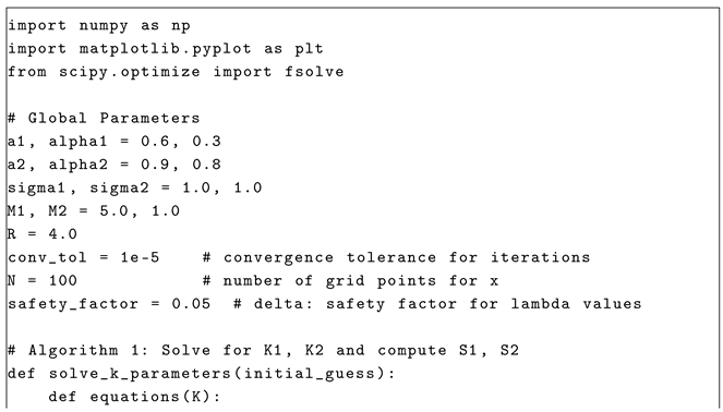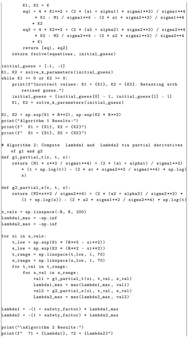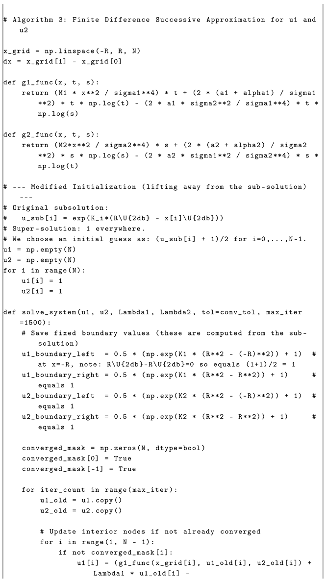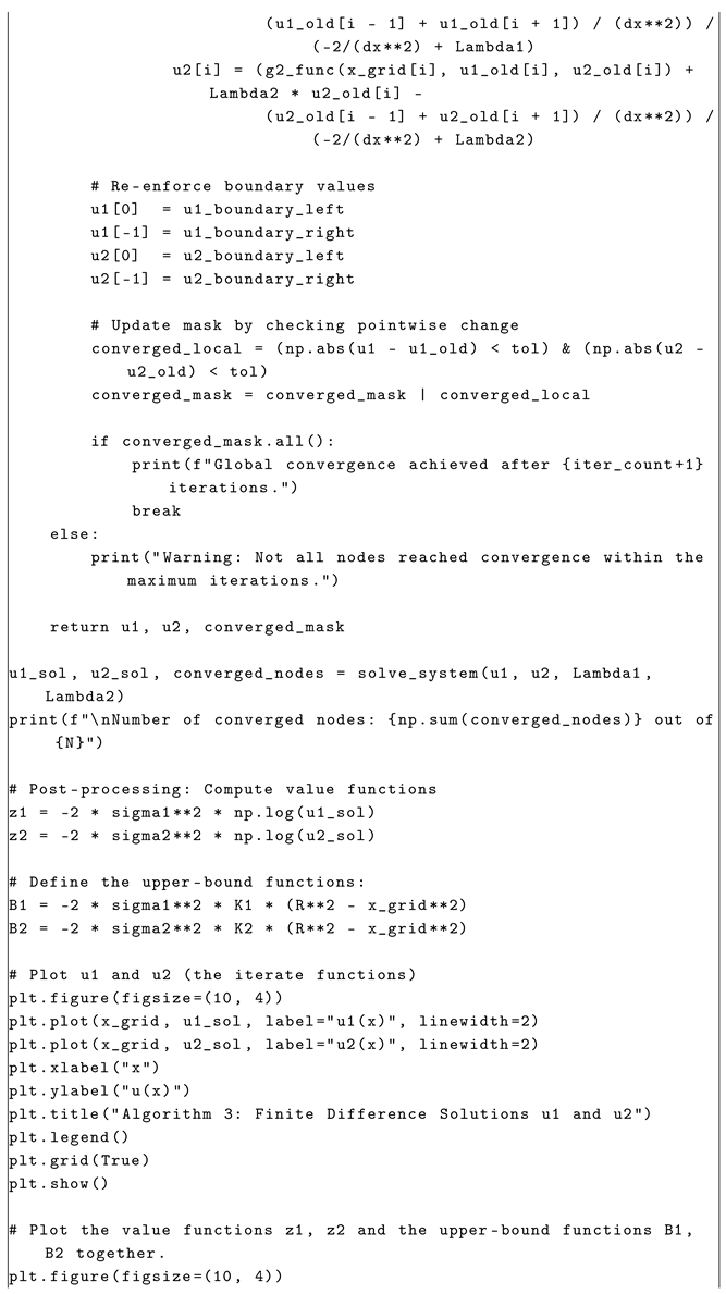Section 7 concludes with the final observations, and Appendix A concludes with a rigorous proof of the key technical result, a detailed presentation of the numerical algorithm implementing our main theorems, and the complete Python (version 3.13.1) code for these computations.

2. Theoretical Framework

In this section, we present the mathematical formulation of the stochastic production planning problem with regime-switching. The model incorporates random demand, regime-dependent parameters, and production controls, as described below.

2.1. Problem Formulation

This paper addresses a stochastic production planning problem involving $D\ge 1$ types of goods stored in inventory with the objective of minimizing production and inventory costs over time under regime-switching economic parameters. The overall criterion is based on a quadratic cost functional that represents the production and holding costs (adjusted for stochastic demand), with production ceasing when inventory levels exceed a given threshold $R>0$. In our model, regimes are characterized by a Markov chain that captures probabilistic transitions between states, and a D-dimensional Brownian motion models stochastic fluctuations in demand.

The stochastic dynamics of the inventory levels are governed by

$$d{y}_i(t,ϵ\left(t\right))=p_i(t,ϵ\left(t\right))dt+{\sigma }_{ϵ\left(t\right)}d{w}_i\left(t\right),y_i(0,ϵ\left(0\right))=y_i^{0,ϵ\left(0\right)},i=1,\dots ,D,$$

(1)

where $p_i$ is the deterministic production rate, $y_i(t,ϵ\left(t\right))$ is an Itô process in $\mathbb{R}$, ${\sigma }_{ϵ\left(t\right)}$ is the regime-dependent volatility, and $ϵ\left(t\right)$ is a Markov chain representing economic regimes (here with two states, but the methodology extends seamlessly to scenarios involving any number of states).

The cost functional is defined as

$$J(p_1,\dots ,p_D)=\mathbb{E}{\int }_0^{\tau }\left(\sum _{i=1}^D{p}_i^2(t,ϵ\left(t\right))+f_{ϵ\left(t\right)}\left(y(t,ϵ\left(t\right))\right)\right)e^{-{\alpha }_{ϵ\left(t\right)}t}dt,$$

subject to the dynamics in (1) and the stopping time $\tau$, which stops production when the inventory exceeds the threshold $R>0$.

2.2. Regime-Switching and Dynamics

We consider a probability space $(\Omega ,\mathcal{F},P)$ together with a standard ${\mathbb{R}}^D$-valued Brownian motion

$$w=\{w_t:t\ge 0\}$$

and an observable finite-state continuous-time homogeneous Markov chain, with states

$$ϵ\left(t\right)=\{{ϵ}_t:t\ge 0\}.$$

We denote by $\mathcal{F}=\{{\mathcal{F}}_t:t\ge 0\}$ the P-augmentation of the filtration $\{\mathcal{F}{(w,ϵ)}_t:t\ge 0\}$ generated by the Brownian motion and the Markov chain, where

$$\mathcal{F}{(w,\epsilon )}_t:=\sigma \left(\{w_s,{ϵ}_s:0\le s\le t\}\right)\mathrm{for}\mathrm{every}t\ge 0.$$

The manager of a firm wants to control the inventory of a given item. We assume a stochastic production environment driven by two sources of randomness:

• Markov Chain: A continuous-time homogeneous Markov chain $ϵ\left(t\right)$, with states $\{1,2\}$, represents economic regimes. These regimes may correspond to scenarios such as economic growth ($ϵ\left(t\right)=1$) or recession ($ϵ\left(t\right)=2$).
• Brownian Motion: A D-dimensional Brownian motion $w\left(t\right)=(w_1\left(t\right),\dots ,w_D\left(t\right))$ models stochastic demand fluctuations in inventory levels.

We also assume that $ϵ$ and w are independent (i.e., HJB system has no “mixed” terms; see [12]), and that the Markov chain $ϵ$ has a strongly irreducible generator, which is given by

$$A=\left[\begin{array}{cc}-a_1& a_1\\ a_2& -a_2\end{array}\right],(\mathrm{transition}\mathrm{rate}\mathrm{matrix}\mathrm{of}\mathrm{the}\mathrm{Markov}\mathrm{chain}ϵ\left(t\right))$$

where $a_1>0$ and $a_2>0$. In this case,

$$\mathrm{if}{p}_t\left(t\right)=E\left[ϵ\left(t\right)\right]\in {\mathbb{R}}^2\mathrm{then}{\displaystyle \frac{d{p}_t\left(t\right)}{dt}}=Aϵ\left(t\right),$$

and $ϵ\left(t\right)$ is explicitly described by the integral form

$$ϵ\left(t\right)=ϵ\left(0\right)+{\int }_0^{t}Aϵ\left(s\right)ds+M\left(t\right),$$

where $M\left(t\right)$ is a martingale with respect to $\mathcal{F}$.

2.3. Inventory Dynamics and State Variables

Let $y_i\left(t\right)$ denote the inventory levels of good i at time t, adjusted for demand, and let $p_i(t,ϵ\left(t\right))$ denote the production rate (control variable) for good i at time t under regime $ϵ\left(t\right)$. The stochastic dynamics of the inventory are governed by

$$d{y}_i\left(t\right)=p_i(t,ϵ\left(t\right))dt+{\sigma }_{ϵ\left(t\right)}d{w}_i\left(t\right),y_i\left(0\right)=y_i^0,i=1,\dots ,D,$$

(2)

where ${\sigma }_{ϵ\left(t\right)}$ is the regime-dependent volatility, $w_i\left(t\right)$ is the i-th component of a D-dimensional Brownian motion, $ϵ\left(t\right)$ is a Markov chain representing economic regimes, and $y_i^0$ denotes the initial inventory level of good i.

2.4. Objective Function

The objective of the stochastic production planning problem is to minimize the total expected cost incurred over time. These costs include both production costs and inventory holding costs, adjusted for regime-switching dynamics and exponential discounting. This is formalized through the following components.

2.4.1. Production Costs

The cost associated with the production rate $p_i(t,ϵ\left(t\right))$ for good i is quadratic and regime-dependent. The quadratic form ensures tractability in optimization and is expressed as

$$C_p\left(t\right)=\sum _{i=1}^D{p}_i^2(t,ϵ\left(t\right)),$$

where $p_i(t,ϵ\left(t\right))$ represents the net production rate (actual production minus demand).

2.4.2. Inventory Costs

The holding cost for storing the inventory is modeled as a convex function of the inventory levels. It accounts for regime-switching parameters and is given by

$$C_h\left(t\right)=f_{ϵ\left(t\right)}\left(y(t,ϵ\left(t\right))\right),$$

where $f_{ϵ\left(t\right)}(·)$ represents regime-dependent holding costs. The convexity of $f_{ϵ\left(t\right)}(·)$ reflects the increasing marginal cost of holding excess inventory.

2.4.3. Discount Factor

To account for the time value of money, the costs are exponentially discounted with a regime-dependent discount rate ${\alpha }_{ϵ\left(t\right)}$. The discount factor ensures that costs incurred in the future are valued less than those incurred immediately.

2.4.4. Cost Functional

The factory aims to minimize production and inventory costs, subject to the stochastic dynamics (2) described above. The total cost functional—combining production costs, inventory costs, and exponential discounting—is given by

$$J(p_1,\dots ,p_D)=\mathbb{E}\left[{\int }_0^{\tau }\left(\sum _{i=1}^D{p}_i^2(t,ϵ\left(t\right))+f_{ϵ\left(t\right)}\left(y(t,ϵ\left(t\right))\right)\right)e^{-{\alpha }_{ϵ\left(t\right)}t}dt\right],$$

where $p_i(t,ϵ\left(t\right))$ is the production rate for good i at time t under regime $ϵ\left(t\right)$; $p_i^2(t,ϵ\left(t\right))$ is the quadratic production cost for good i; ${\sum }_{i=1}^D{p}_i^2(t,ϵ\left(t\right))$ is the regime-dependent production costs, modeled as quadratic functions of the production rate; $y(t,ϵ(t\left)\right)$ represents the inventory levels of goods, adjusted for demand; $f_{ϵ\left(t\right)}\left(y(t,ϵ\left(t\right))\right)$ represents the regime-dependent inventory holding costs (holding cost, modeled as convex functions $f_1\left(x\right)$ and $f_2\left(x\right)$); and ${\alpha }_{ϵ\left(t\right)}$ is the regime-dependent discount rate for exponential discounting.

The stopping time $\tau$ is defined as the moment when the inventory exceeds an exogenous threshold R, i.e.,

$$\tau =inf\{t>0:\parallel y(t,ϵ\left(t\right))\parallel \ge R\},y(t,ϵ\left(t\right))=\left(y_1(t,ϵ\left(t\right)),...,y_D(t,ϵ\left(t\right))\right),$$

where $∥\circ ∥$ stands for the Euclidian norm.

3. Optimization Problem

The primary objective of the stochastic production planning problem is to minimize the total expected cost, which comprises both production and inventory holding costs, subject to the constraints of stochastic inventory dynamics and regime-switching parameters. This optimization problem is formulated as follows.

3.1. Optimization Objective

The objective is to determine the optimal production rates $p_1(t,ϵ\left(t\right))$, …, $p_D(t,ϵ\left(t\right))$ that minimize the total cost functional J, while satisfying the stochastic inventory dynamics. Mathematically, this is expressed as

$$\underset{p(t,ϵ\left(t\right))\in {\mathbb{R}}^D}{inf}J\left(p(t,ϵ\left(t\right))\right),p(t,ϵ\left(t\right))=\left(p_1(t,ϵ\left(t\right)),\dots ,p_D(t,ϵ\left(t\right))\right)$$

subject to the inventory dynamics:

$$d{y}_i\left(t\right)=p_i(t,ϵ\left(t\right))dt+{\sigma }_{ϵ\left(t\right)}d{w}_i\left(t\right),y_i\left(0\right)=y_i^0,i=1,\dots ,D.$$

The optimization problem is solved over a finite horizon, up to the stopping time $\tau$, and incorporates the effects of regime-switching. The constraints ensure that the optimization respects the stochastic nature of the inventory dynamics and the stopping criterion at $\tau$.

3.2. Hamilton–Jacobi–Bellman Equations

To solve the optimization problem, we employ the value function approach. The value function is defined as

$$z_i\left(x\right)=\underset{p_1,\dots ,p_D}{inf}\mathbb{E}\left[{\int }_0^{\tau }\left(\sum _{j=1}^D{p}_j^2(t,ϵ\left(t\right))+f_{ϵ\left(t\right)}\left(y(t,ϵ\left(t\right))\right)\right)e^{-{\alpha }_{ϵ\left(t\right)}t}dt|y\left(0\right)=x,ϵ\left(0\right)=i\right].$$

(3)

The HJB equations for the value functions $z_1\left(x\right)$ and $z_2\left(x\right)$, corresponding to the two regimes $ϵ\left(t\right)=1$ and $ϵ\left(t\right)=2$, are given by

$$\left\{\begin{array}{ccc}-a_1{z}_2+(a_1+{\alpha }_1)z_1-{\displaystyle \frac{{{\sigma }_1}^2}{2}}\Delta z_1-f_1\left(x\right)=-{\displaystyle \frac{1}{4}}{\left|\nabla z_1\right|}^2,& \mathrm{for}& x\in B_R,\\ -a_2{z}_1+(a_2+{\alpha }_2)z_2-{\displaystyle \frac{{{\sigma }_2}^2}{2}}\Delta z_2-f_2\left(x\right)=-{\displaystyle \frac{1}{4}}{\left|\nabla z_2\right|}^2,& \mathrm{for}& x\in B_R,\end{array}\right.$$

(4)

with the following boundary conditions:

$$z_1\left(x\right)=z_2\left(x\right)=0,\mathrm{for}x\in \partial B_R.$$

Here, $a_1,a_2,{\alpha }_1,{\alpha }_2,{\sigma }_1,{\sigma }_2$ are regime-dependent parameters, $\Delta z_i$ is the Laplacian of $z_i\left(x\right)$ (sum of second-order partial derivatives), $B_R$ is the open ball in ${\mathbb{R}}^D$ ($D\ge 1$) of radius $R>0$, and $f_1\left(x\right)$ and $f_2\left(x\right)$ are the holding cost functions in regimes 1 and 2, respectively.

Assumptions

To ensure mathematical tractability, we impose the following assumptions:

• $f_1\left(x\right)$ and $f_2\left(x\right)$ are continuous, convex functions satisfying $f_i\left(x\right)\le M_i{∥x∥}^2$, $i=1,2$;
• ${\sigma }_{ϵ\left(t\right)}>0$ and ${\alpha }_{ϵ\left(t\right)}>0$, ensuring non-degenerate stochastic dynamics;
• Boundary conditions: $z_{ϵ\left(t\right)}=0$ when $t=\tau$, $i=1,\dots ,D$.

The hypotheses on $f_1$ and $f_2$ are chosen so that

$$z_i\left(y\right)\le C\left(1+{\parallel y\parallel }^2\right)\mathrm{for}\mathrm{some}C>0,$$

and so that the running cost $J(y,p)$ is convex in $(y,p)$. Together, these conditions guarantee that each value–function $z_i$ is convex in y.

This formulation provides the mathematical foundation for deriving the Hamilton–Jacobi–Bellman equations and solving the optimization problem.

The computational goal is to approximate the value functions $z_1\left(x\right)$ and $z_2\left(x\right)$ using numerical techniques that guarantee convergence and stability.

The next section focuses on the methodology used to obtain the solutions.

3.3. Transformation and Simplification

To simplify the PDE system (4), we apply a change in variables: $z_j\left(x\right)=-2{\sigma }_j^{2}ln{u}_j\left(x\right),$$j=1,2,$ which removes the gradient terms and transforms the PDE system into

$$\left\{\begin{array}{ccc}\Delta u_1\left(x\right)=u_1\left(x\right)\left[{\displaystyle \frac{1}{{\sigma }_1^4}}{f}_1\left(x\right)+{\displaystyle \frac{2(a_1+{\alpha }_1)}{{\sigma }_1^2}}ln{u}_1\left(x\right)-2a_1{\displaystyle \frac{{\sigma }_2^2}{{\sigma }_1^4}}ln{u}_2\left(x\right)\right],& for& x\in B_R\\ \Delta u_2\left(x\right)=u_2\left(x\right)\left[{\displaystyle \frac{1}{{\sigma }_2^4}}{f}_2\left(x\right)+{\displaystyle \frac{2(a_2+{\alpha }_2)}{{\sigma }_2^2}}ln{u}_2\left(x\right)-2a_2{\displaystyle \frac{{\sigma }_1^2}{{\sigma }_2^4}}ln{u}_1\left(x\right)\right],& for& x\in B_R\end{array}\right.$$

(5)

with the following boundary conditions:

$$u_1\left(x\right)=u_2\left(x\right)=1,x\in \partial B_R.$$

This transformation reduces the complexity of the system and facilitates numerical computation.

3.4. Existence and Uniqueness of Solutions

The solution’s computation involved specific parameters that had to be determined in an approximately exact form. In the paper [8], we established only the existence of these parameters. Therefore, it becomes essential to provide a proof of the results that will facilitate our computational technique. Consequently, to facilitate the implementation of our main results, we state the following practical lemma; its proof can be found in Appendix A.1.

Lemma 1.

For any $a_1,{\alpha }_1,a_2,{\alpha }_2,{\sigma }_1,{\sigma }_2,M_1,M_2,R\in (0,\infty )$, and $D\in {\mathbb{N}}^{*}$, there exist unique $K_1,K_2\in (-\infty ,0)$ such that

$$\left\{\begin{array}{c}4K_1^2+{\displaystyle \frac{2(a_1+{\alpha }_1){\sigma }_1^2}{{\sigma }_1^4}}{K}_1-{\displaystyle \frac{M_1}{{\sigma }_1^4}}-{\displaystyle \frac{2a_1{\sigma }_2^2}{{\sigma }_1^4}}{K}_2=0,\hfill \\ 4K_2^2+{\displaystyle \frac{2(a_2+{\alpha }_2){\sigma }_2^2}{{\sigma }_2^4}}{K}_2-{\displaystyle \frac{M_2}{{\sigma }_2^4}}-{\displaystyle \frac{2a_2{\sigma }_1^2}{{\sigma }_2^4}}{K}_1=0,\hfill \\ -{\displaystyle \frac{2(a_1+{\alpha }_1)R^2}{{\sigma }_1^2}}{K}_1-2D{K}_1+{\displaystyle \frac{2a_1{\sigma }_2^2{R}^2}{{\sigma }_1^4}}{K}_2\ge 0,\hfill \\ -{\displaystyle \frac{2(a_2+{\alpha }_2)R^2}{{\sigma }_2^2}}{K}_2-2D{K}_2+{\displaystyle \frac{2a_2{\sigma }_1^2{R}^2}{{\sigma }_2^4}}{K}_1\ge 0.\hfill \end{array}\right.$$

(6)

We are now ready to adapt the proof of the theorem in [8], integrating the necessary steps to address the numerical implications.

Theorem 1.

Let $K_1,K_2\in \left(-\infty ,0\right)$ be the unique solutions of the nonlinear system (6):

$$B_1\left(x\right)=-2{\sigma }_1^2{K}_1(R^2-{\left|x\right|}^2)and{B}_2\left(x\right)=-2{\sigma }_2^2{K}_2(R^2-{\left|x\right|}^2).$$

The system of Equation (4) has a unique positive convex solution $(z_1,z_2)\in {[C^2\left(B_R\right)\cap C\left({\overline{B}}_R\right)]}^2$ with value functions $z_1$ and $z_2$ such that

$$z_1\left(x\right)\le B_1\left(x\right)\mathrm{and}{z}_2\left(x\right)\le B_2\left(x\right),\mathrm{for}\mathrm{all}x\in {\overline{B}}_R.$$

Proof. 

Our constructive approach aims to develop a computational scheme for numerical approximations of the solution. Since the system (4) is equivalent to (5), we will focus on the latter. The approach involves four key steps.

• Step 1: Sub-solution and Super-solution Construction.

The main problem reduces to constructing functions $(u_1,u_2)$ as sub-solutions (and $(u_1,u_2)$ as super-solutions) for the system (5) that satisfy the following inequalities:

$$\left\{\begin{array}{ccc}\Delta u_1\left(x\right)\ge u_1\left(x\right)\left[{\displaystyle \frac{1}{{\sigma }_1^4}}{f}_1\left(x\right)+{\displaystyle \frac{2(a_1+{\alpha }_1)}{{\sigma }_1^2}}ln{u}_1\left(x\right)-{\displaystyle \frac{2a_1{\sigma }_2^2}{{\sigma }_1^4}}ln{u}_2\left(x\right)\right],\hfill & for\hfill & x\in B_R,\hfill \\ \Delta u_2\left(x\right)\ge u_2\left(x\right)\left[{\displaystyle \frac{1}{{\sigma }_2^4}}{f}_2\left(x\right)+{\displaystyle \frac{2(a_2+{\alpha }_2)}{{\sigma }_2^2}}ln{u}_2\left(x\right)-{\displaystyle \frac{2a_2{\sigma }_1^2}{{\sigma }_2^4}}ln{u}_1\left(x\right)\right],\hfill & for\hfill & x\in B_R,\hfill \\ (u_1\left(x\right),u_2\left(x\right))=\left(1,1\right),\hfill & for\hfill & x\in \partial B_R,\hfill \end{array}\right.$$

(and similarly for the inequalities with ≤). For sub-solutions, choose

$$({\underline{u}}_1\left(x\right),{\underline{u}}_2\left(x\right))=\left(e^{K_1(R^2-{\left|x\right|}^2)},e^{K_2(R^2-{\left|x\right|}^2)}\right),$$

where

$$K_1,K_2\in (-\infty ,0),$$

are solutions of (6). For super-solutions, choose

$$({\overline{u}}_1\left(x\right),{\overline{u}}_2\left(x\right))=(1,1).$$

Clearly,

$${\underline{u}}_1\left(x\right)\le {\overline{u}}_1\left(x\right)\mathrm{and}{\underline{u}}_2\left(x\right)\le {\overline{u}}_2\left(x\right),\mathrm{for}\mathrm{any}x\in {\overline{B}}_R.$$

Step 2: Approximation Scheme.

Construct sequences ${\left\{(u_1^k,u_2^k)\right\}}_{k\in \mathbb{N}}$ via monotone Picard iterations, starting with

$$(u_1^0,u_2^0)=({\overline{u}}_1,{\overline{u}}_2),x\in {\overline{B}}_R.$$

Define the iteration

$$\left\{\begin{array}{ccc}\Delta u_1^k+{\Lambda }_1{u}_1^k=g_1(x,u_1^{k-1},u_2^{k-1})+{\Lambda }_1{u}_1^{k-1},& for& x\in B_R,\\ \Delta u_2^k+{\Lambda }_2{u}_2^k=g_2(x,u_1^{k-1},u_2^{k-1})+{\Lambda }_2{u}_2^{k-1},& for& x\in B_R,\end{array}\right.$$

where for

$$S_1=e^{K_1{R}^2},S_2=e^{K_2{R}^2},\mathrm{and}S=1,$$

the functions

$$g_1:{\overline{B}}_R\times [S_1,S]\times [S_2,S]\to \mathbb{R}\mathrm{and}{g}_2:{\overline{B}}_R\times [S_2,S]\times [S_1,S]\to \mathbb{R}$$

are defined by

$$\begin{array}{ccc}\hfill g_1\left(x,t,s\right)& =& {\displaystyle \frac{1}{{\sigma }_1^4}}{f}_1\left(x\right)t+{\displaystyle \frac{2(a_1+{\alpha }_1)}{{\sigma }_1^2}}tlnt-{\displaystyle \frac{2a_1{\sigma }_2^2}{{\sigma }_1^4}}tlns,\hfill \\ & & \hfill \\ \hfill g_2\left(x,t,s\right)& =& {\displaystyle \frac{1}{{\sigma }_2^4}}{f}_2\left(x\right)s+{\displaystyle \frac{2(a_2+{\alpha }_2)}{{\sigma }_2^2}}slns-{\displaystyle \frac{2a_2{\sigma }_1^2}{{\sigma }_2^4}}slnt.\hfill \end{array}$$

(7)

Since $g_1$ (respectively, $g_2$) is a continuous function with respect to the first variable in $B_R$ and continuously differentiable with respect to the second and third in

$$[S_1,S]\times [S_2,S],$$

respectively,

$$[S_2,S]\times [S_1,S],$$

this allows us to choose

$${\Lambda }_1,{\Lambda }_2\in (-\infty ,0)$$

such that

$$-{\Lambda }_1\ge {\displaystyle \frac{g_1\left(x,t_1,s\right)-g_1\left(x,t_2,s\right)}{t_2-t_1}},(={\displaystyle \frac{\partial g_1}{\partial t}}),$$

(8)

respectively

$$-{\Lambda }_2\ge {\displaystyle \frac{g_2\left(x,t,s_1\right)-g_2\left(x,t,s_2\right)}{s_2-s_1}},(={\displaystyle \frac{\partial g_2}{\partial s}}),$$

(9)

for every $t_1,t_2$ with

$${\underline{u}}_1\le t_2<t_1\le {\overline{u}}_1,{\underline{u}}_2\le s\le {\overline{u}}_2\mathrm{and}x\in {\overline{B}}_R,$$

respectively, for every $s_1,s_2$ with

$${\underline{u}}_2\le s_2<s_1\le {\overline{u}}_2,{\underline{u}}_1\le t\le {\overline{u}}_1\mathrm{and}x\in {\overline{B}}_R,$$

to ensure monotonicity

$$(u_1^{k-1}\le u_1^k,u_2^{k-1}\le u_2^k)\Rightarrow (u_1^k\le u_1^{k+1},u_2^k\le u_2^{k+1}),$$

via mathematical induction and the maximum principle.

• Step 3: Convergence and Uniqueness.

The sequences ${\{u_1^k,u_2^k\}}_{k\in \mathbb{N}}$ converge monotonically to bounded limits:

$$\underset{k\to \infty }{lim}(u_1^k\left(x\right),u_2^k\left(x\right))=(u_1\left(x\right),u_2\left(x\right)),x\in {\overline{B}}_R.$$

Standard bootstrap arguments ensure that

$$(u_1^k,u_2^k)\to (u_1,u_2)\mathrm{in}{[C^2\left(B_R\right)\cap C\left({\overline{B}}_R\right)]}^2,$$

and $(u_1,u_2)$ solves (5) with

$${\underline{u}}_1\left(x\right)\le u_1\left(x\right)\le {\overline{u}}_1\left(x\right),{\underline{u}}_2\left(x\right)\le u_2\left(x\right)\le {\overline{u}}_2\left(x\right),x\in {\overline{B}}_R.$$

Uniqueness follows from the maximum principle, i.e., any two positive solutions $(u_1,u_2)$ and $({\tilde{u}}_1,{\tilde{u}}_2)$ coincide.

Step 4: 

Since J is convex in $(y,p)$, the state equation is affine in p, and $z_i$ grows at most quadratically and is continuous, it then follows that the function $z_i$ is convex on ${\mathbb{R}}^D$ (see [8]).

   □

4. Optimal Control

The optimal control represents the production rate policy that minimizes the total expected cost functional. It is derived using the Hamilton–Jacobi–Bellman (HJB) equations and is directly related to the gradients of the value functions. Below, we delve deeper into its formulation and derivation.

4.1. Optimal Production Policy

By differentiating the HJB equations with respect to the inventory levels $y_i$, we obtain the gradient terms that define the optimal control.

Hence, for each economic good $i=1,\dots ,D$, the optimal production rate $p_i^{*}(t,ϵ\left(t\right))$ is given by

$$p_i^{*}(t,ϵ\left(t\right))=-{\displaystyle \frac{1}{2}}{\displaystyle \frac{\partial z_{ϵ\left(t\right)}}{\partial y_i}},$$

where $z_{ϵ\left(t\right)}$ is the value function corresponding to regime $ϵ\left(t\right)$ and ${\displaystyle \frac{\partial z_{ϵ\left(t\right)}}{\partial y_i}}$ denotes the partial derivative of the value function with respect to the inventory level of good i.

This result is obtained by solving the first-order optimality condition derived from the HJB equations.

Economic Interpretation

The negative gradient of the value function implies that the optimal production rate decreases as the marginal cost of inventory increases. Intuitively, higher inventory levels (positive gradient) lead to a reduction in production to avoid excess costs, and lower inventory levels (negative gradient) necessitate an increase in production to meet anticipated demand.

4.2. Verification of Optimality

The verification of optimality establishes that the control $p^{*}(t,ϵ\left(t\right))$, derived from the Hamilton–Jacobi–Bellman (HJB) equations, is indeed the optimal control that minimizes the cost functional. This involves proving the supermartingale property of the value function for all admissible controls and the martingale property for the optimal control.

4.2.1. The Stochastic Process

To verify that $p_i^{*}(t,ϵ\left(t\right))$ is indeed the optimal control, we use the supermartingale and martingale properties of the value function $z_{ϵ\left(t\right)}\left(y\right)$. Let the stochastic process $Z_p\left(t\right)$ be defined as

$$Z_p\left(t\right)=-e^{-{\alpha }_{ϵ\left(t\right)}t}{z}_{ϵ\left(t\right)}\left(y(t,ϵ\left(t\right))\right)-{\int }_0^t\left(\sum _{i=1}^D{p}_i^2(s,ϵ\left(s\right))+f_{ϵ\left(s\right)}\left(y(s,ϵ\left(s\right))\right)\right)e^{-{\alpha }_{ϵ\left(s\right)}s}ds,$$

(10)

where $z_{ϵ\left(t\right)}\left(y\right)$ is the value function for regime $ϵ\left(t\right)$, $p_i(t,ϵ\left(t\right))$ are the production rates (control variables), $f_{ϵ\left(t\right)}\left(y\right)$ is the holding cost function, and ${\alpha }_{ϵ\left(t\right)}$ is the regime-dependent discount rate.

Using Itô’s lemma, the time derivative of $Z_p\left(t\right)$ satisfies

$$d{Z}_p\left(t\right)=e^{-{\alpha }_{ϵ\left(t\right)}t}\left[{\alpha }_{ϵ\left(t\right)}{z}_{ϵ\left(t\right)}\left(y\right)+\mathcal{L}{z}_{ϵ\left(t\right)}\left(y\right)-\sum _{i=1}^D{p}_i^2(t,ϵ\left(t\right))-f_{ϵ\left(t\right)}\left(y\right)\right]dt+M\left(t\right),$$

where $M\left(t\right)$ is a martingale term, and $\mathcal{L}{z}_{ϵ\left(t\right)}\left(y\right)$ represents the generator of the Markov-modulated diffusion (here, the Laplacian operator).

4.2.2. Supermartingale and Martingale Properties

For the admissible controls $p_i(t,ϵ\left(t\right))$, $Z_p\left(t\right)$ is a supermartingale because $\mathcal{L}L{z}_{ϵ\left(t\right)}\left(y\right)$ satisfies the following HJB inequality:

$${\alpha }_{ϵ\left(t\right)}{z}_{ϵ\left(t\right)}\left(y\right)+\mathcal{L}{z}_{ϵ\left(t\right)}\left(y\right)-\sum _{i=1}^D{p}_i^2(t,ϵ\left(t\right))-f_{ϵ\left(t\right)}\left(y\right)\le 0.$$

For the optimal control $p^{*}(t,ϵ\left(t\right))$, $\mathcal{L}{Z}_p\left(t\right)$ is a martingale because $L{z}_{ϵ\left(t\right)}\left(y\right)$ satisfies the equality condition:

$${\alpha }_{ϵ\left(t\right)}{z}_{ϵ\left(t\right)}\left(y\right)+\mathcal{L}{z}_{ϵ\left(t\right)}\left(y\right)-\sum _{i=1}^D{p}_i^{*2}(t,ϵ\left(t\right))-f_{ϵ\left(t\right)}\left(y\right)=0.$$

The optimal control $p^{*}(t,ϵ\left(t\right))$ ensures that $Z_p\left(t\right)$ is a martingale, while any other control $p(t,ϵ(t\left)\right)$ results in $Z_p\left(t\right)$ being a supermartingale. This validates the optimality of $p^{*}(t,ϵ\left(t\right))$.

4.2.3. Boundary Conditions and Optimality

The boundary condition

$$z_{ϵ\left(t\right)}\left(y\right)=0\mathrm{for}y\in \partial B_R,$$

where $B_R$ is the ball of radius R, which ensures that $Z_p\left(t\right)$ vanishes at the stopping time $\tau$. Thus, for $t\ge \tau$, the contribution to the cost functional ceases, confirming the proper termination of production when inventory exceeds the threshold R.

The optimality of $p^{*}(t,ϵ\left(t\right))$ is formalized through the following theorem:

Theorem 2.

Let $Z_p\left(t\right)$ be the stochastic process defined in (10). The control $p^{*}(t,ϵ\left(t\right))$, derived from the HJB equations, minimizes the cost functional $J\left(p_1,\dots ,p_D\right)$ and satisfies

$$Z_{p^{*}}\left(t\right)=z_{ϵ\left(t\right)}\left(y\left(0\right)\right).$$

Proof. 

• For $Z_p\left(t\right)$ under the admissible control $p(t,ϵ(t\left)\right)$,

  $$\mathbb{E}\left[Z_p\left(\tau \right)\right]\le Z_p\left(0\right),$$

  since $Z_p\left(t\right)$ is a supermartingale.
• For $Z_{p^{*}}\left(t\right)$ under the optimal control $p^{*}(t,ϵ\left(t\right))$,

  $$\mathbb{E}\left[Z_{p^{*}}\left(\tau \right)\right]=Z_{p^{*}}\left(0\right),$$

  since $Z_{p^{*}}\left(t\right)$ is a martingale.
• From the boundary condition $z_{ϵ\left(t\right)}\left(y\right)=0$, it follows that

  $$\mathbb{E}\left[{\int }_0^{\tau }\left(\sum _{i=1}^D{p}_i^2(s,ϵ\left(s\right))+f_{ϵ\left(s\right)}\left(y(s,ϵ\left(s\right))\right)\right)e^{-{\alpha }_{ϵ\left(s\right)}s}ds\right]=z_{ϵ\left(t\right)}\left(y\left(0\right)\right).$$
  Thus, the control $p^{*}(t,ϵ\left(t\right))$ minimizes the cost functional $J(p_1,\dots ,p_D)$ and satisfies the optimality condition.

   □

4.2.4. Theoretical Properties of the Optimal Control and Inventory Process

The theoretical properties of the optimal control are as follows: the optimal control $p_i^{*}(t,ϵ\left(t\right))$ is Lipschitz continuous in y, ensuring stability in production rates under small changes in inventory levels; the control policy is adaptive, responding dynamically to regime changes governed by the Markov chain $ϵ\left(t\right)$; and the quadratic nature of the cost functional guarantees uniqueness of the optimal control.

The inventory process is modeled by the stochastic differential equation (SDE)

$$dy\left(t\right)=p^{*}(t,\epsilon \left(t\right))dt+{\sigma }_{\epsilon \left(t\right)}dW\left(t\right),y\left(0\right)=x_0\in {\mathbb{R}}^D,$$

where the economic regime $\epsilon \left(t\right)$ takes the values $\{1,2\}$ with the following transitions:

$$\mathbb{P}(\epsilon (t+dt)=2\mid \epsilon \left(t\right)=1)=a_{1}dt\mathrm{and}\mathbb{P}(\epsilon (t+dt)=1\mid \epsilon \left(t\right)=2)=a_{2}dt.$$

In the simulation, one uses a time step $\Delta t$ and performs the following update:

$$y(t+\Delta t)=y\left(t\right)+p^{*}(y\left(t\right),ϵ\left(t\right))\Delta t+{\sigma }_{ϵ\left(t\right)}\sqrt{\Delta t}\xi ,$$

where $\xi$ is an independent standard normal random variable. The optimal control is obtained by interpolating the computed value function gradients:

$$p_i^{*}(y,ϵ\left(t\right))=-{\displaystyle \frac{1}{2}}{\displaystyle \frac{\partial z_{ϵ\left(t\right)}}{\partial y_i}},(i=1,\dots ,D,ϵ\left(t\right)\in \{1,2\}),$$

where $z_{ϵ\left(t\right)=1}=z_1$ and $z_{ϵ\left(t\right)=2}=z_2$ solve the coupled HJB system in each regime.

The simulation by Euler–Maruyama is executed until the stopping time

$$\tau =inf\{t>0:|y\left(t\right)|\ge R\},$$

at which point the production is halted.

5. Sensitivity, Model Analysis, and Visualization

The proof of the results in this section is detailed in reference [8], and thus, the specifics are excluded here. The data are presented for its visualization in accordance with the results, showcasing the strength of the mathematical conclusions and numerical implementation.

5.1. Sensitivity Analysis

The sensitivity analysis shows the following impacts:

Theorem 3.

If ${\alpha }_1={\alpha }_2$ and $f_1\left(x\right)=f_2\left(x\right)$, for all $x\in B_R$, then higher volatility (${\sigma }_1>{\sigma }_2$) increases the following value function:

$$z_1\left(x\right)\ge z_2\left(x\right)forallx\in {\overline{B}}_R.$$

Theorem 4.

If ${\sigma }_1={\sigma }_2$ and $f_1\left(x\right)=f_2\left(x\right)$, for all $x\in B_R$, then higher discount rates (${\alpha }_1<{\alpha }_2$) decrease the value function

$$z_1\left(x\right)\ge z_2\left(x\right),forallx\in {\overline{B}}_R.$$

Theorem 5.

If ${\alpha }_1={\alpha }_2$ and ${\sigma }_1={\sigma }_2$, then higher holding costs ($f_1\left(x\right)>f_2\left(x\right)$) increase the value function

$$z_1\left(x\right)\ge z_2\left(x\right),forallx\in {\overline{B}}_R.$$

5.2. Model Comparisons

For models with and without regime-switching, we have

Theorem 6.

If ${\sigma }_1>{\sigma }_2$, ${\alpha }_1<{\alpha }_2$, and $f_1\left(x\right)>f_2\left(x\right)$, for all $x\in B_R$, then

$${\overline{z}}_1\left(x\right)\ge z_1\left(x\right)\ge z_2\left(x\right)\ge {\underline{z}}_2\left(x\right),forallx\in B_R,$$

where ${\overline{z}}_1\left(x\right)$ and ${\underline{z}}_2\left(x\right)$ correspond to the value functions of a model without regime-switching.

5.3. Visualization of the Solution in the Case $D=1$

In this section, we connect our theoretical results (Theorems 3–6) with concrete numerical experiments in the case $D=1$. We first present a compact tabular summary of the sensitivity analysis statements, then illustrate the transformed solutions and value functions, and finally show the time dynamics of the optimal control and inventory. All plots were generated with the annotated Python code in Appendix A.3, which can be adapted to other parameter choices so long as the monotonicity and convergence assumptions remain valid.

5.3.1. Summary of Sensitivity Results

Table 1. Effects of parameter variations on value functions $z_1,z_2$.

Theorem	Parameter Change	Effect on ${\mathit{z}}_{\mathit{i}}\left(\mathit{x}\right)$, $\mathit{x}\in {\overline{\mathit{B}}}_{\mathit{R}}$
3	${\sigma }_1>{\sigma }_2$	Higher volatility raises $z_1\ge z_2$.
4	${\alpha }_1<{\alpha }_2$	Lower discount rate raises $z_1\ge z_2$.
5	$f_1\left(x\right)>f_2\left(x\right)$	Higher holding cost raises $z_1\ge z_2$.
6	all above+switching limits	Yields ${\overline{z}}_1\ge z_1\ge z_2\ge {\underline{z}}_2$.

collects the four main sensitivity comparisons of Section 5.1, restating the impact of parameter changes on the regime-dependent value functions.

Next, we give a concise workflow diagram, which summarize the sensitivity statements in tabular form.

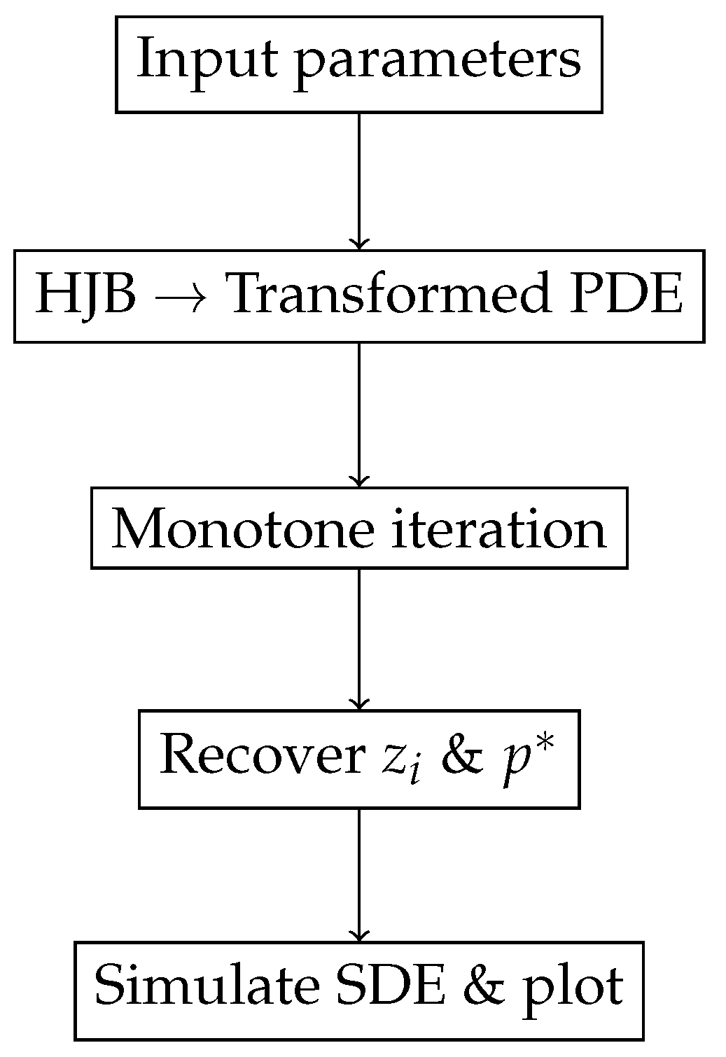
5.3.2. Workflow Overview

• Model specification ($\{a_i,{\alpha }_i,M_i,{\sigma }_i,f_i\}$).
• HJB PDE derivation and logarithmic transform $z_i\mapsto u_i$.
• Monotone iteration (Picard) for $(u_1,u_2)$ on ${\overline{B}}_R$.
• Back-transform to obtain $z_1$, $z_2$ and compute feedback law $p^{*}\left(y\right)$.
• Simulate inventory SDE under optimal control and regime-switching.

Figure 1 depicts the end-to-end computational pipeline:

We now present four detailed case studies “one per theorem” each with its own parameter table, plots, and discussion of practical relevance.

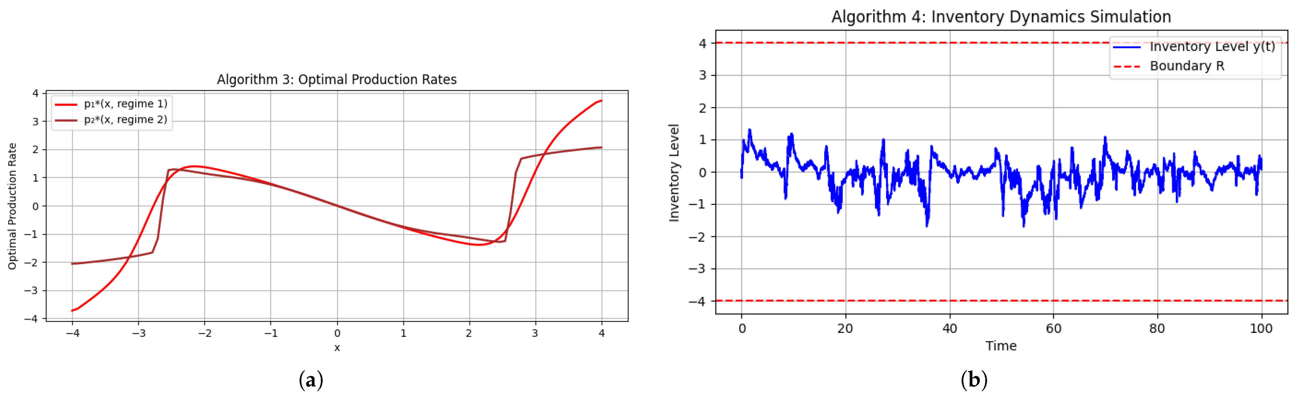
5.3.3. Case Study: Volatility Variation (Theorem 3)

To connect our theoretical model with practical applications (see [4]), we vary certain parameters that typically arise in real-world problems.

Table 2. Parameters for Theorem 3 experiment.

Parameter	Regime 1	Regime 2
$a_i$	0.6	0.5
${\alpha }_i$	0.3	0.3
$M_i$	1	1
${\sigma }_i$	0.9	0.2
$f_i\left(x\right)$	$x^2$	$x^2$
R	4

lists these inputs.

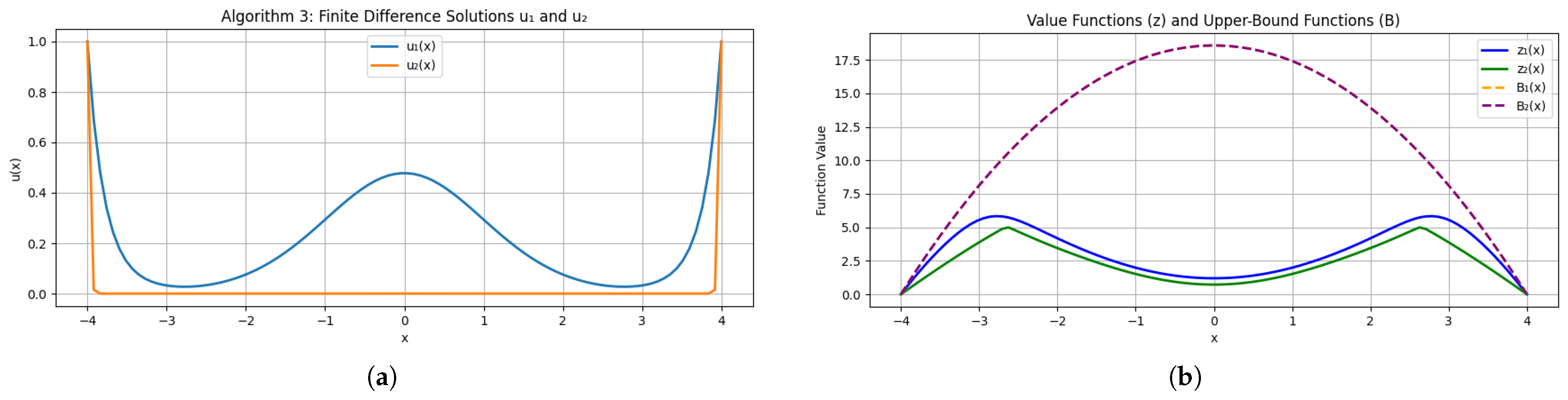
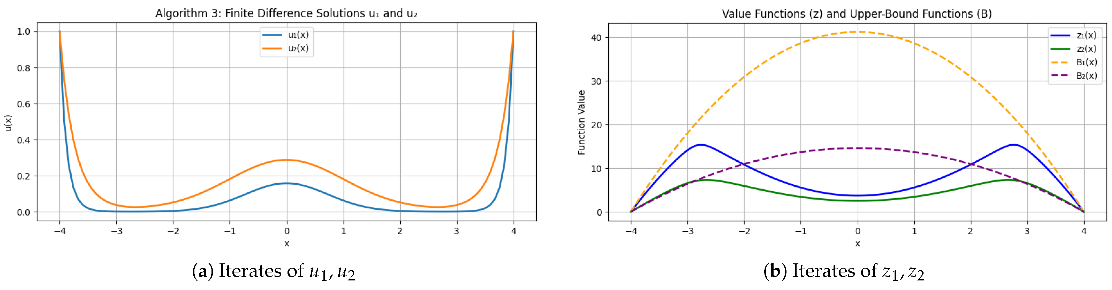
Figure 2a,b show the numerically computed transformed solutions $u_1,u_2$ (so that $z_i=-{\displaystyle \frac{2}{{\sigma }_i^2}}{K}_{i}ln{u}_i$) alongside the regime-dependent value functions.

This choice satisfies the hypotheses of Theorem 3 and ensures that volatility differences dominate the ordering of $z_1$ and $z_2$.

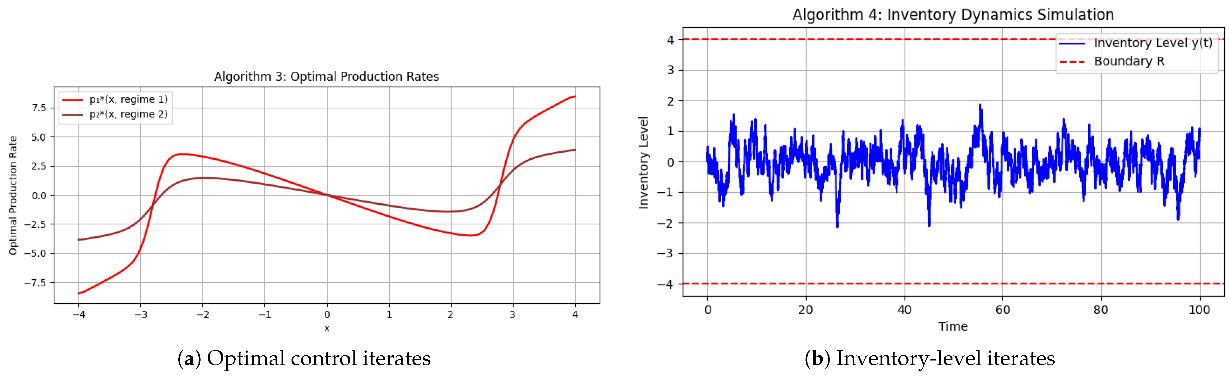
Figure 3a,b display a sample path under one realization of the regime-switching process.

Interpretation

In a microgrid context, $a_i$ and ${\sigma }_i$ model drift and renewable generation uncertainty, while $f_i\left(x\right)=x^2$ penalizes inventory deviations. Theorem 3 predicts $z_1\ge z_2$ when ${\sigma }_1>{\sigma }_2$, confirmed by both the static profiles and dynamic simulation. The negative $K_i$ and ${\Lambda }_i$ ensure convexity and damping in the transformed PDEs (see Lemma 1 and Theorem 1).

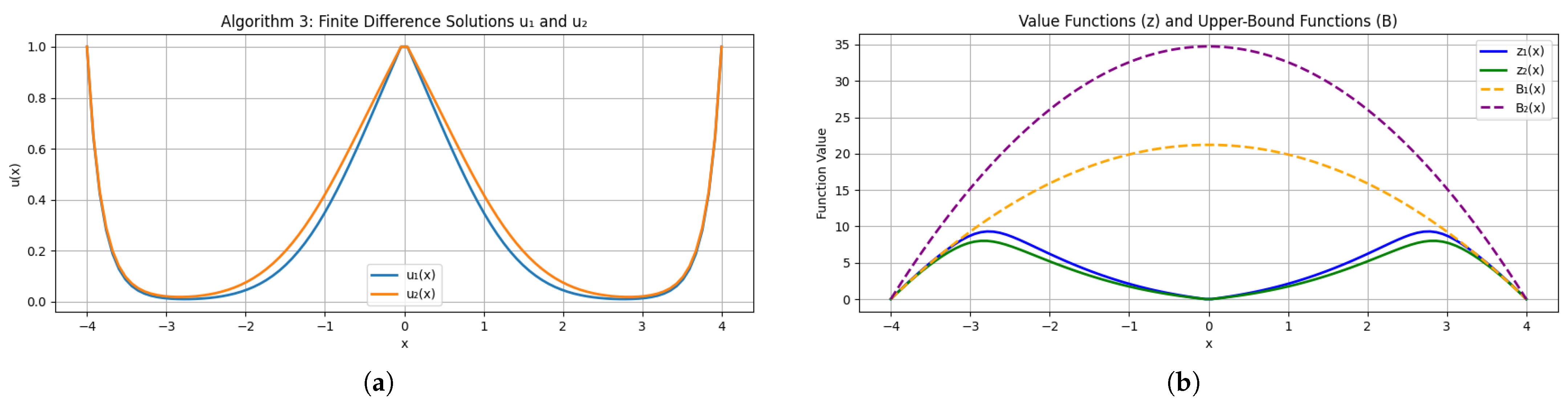
5.3.4. Case Study: Discount Rate Variation (Theorem 4)

To illustrate Theorem 4, we choose parameters motivated by a multi-product, multi-machine manufacturing setting [5] (

Table 3. Parameter set for Theorem 4 experiment.

Parameter	Regime 1	Regime 2	Interpretation
$a_i$	$0.6$	$0.9$	Regime-switching rates
${\alpha }_i$	$0.2$	$0.9$	Discount factors (${\alpha }_1<{\alpha }_2$)
$M_i$	2	2	Bound on $f_i\left(x\right)$
${\sigma }_i$	1	1	Common volatility
$f_i\left(x\right)$	$2x^2$		Quadratic holding cost
Domain	$x\in {\overline{B}}_4$		Inventory threshold $R=4$

).

Figure 4a,b plot the transformed variables $u_1$, $u_2$ and the resulting value functions $z_1$, $z_2$ along a radial slice in ${\overline{B}}_4$.

Notice $z_1\ge z_2$ throughout, confirming the result in Theorem 4 (Figure 5).

Interpretation

The lower discount rate in regime 1 increases the present value of future costs, driving $z_1$ above $z_2$ in line with Theorem 4. The parameters $a_i$ and ${\alpha }_i$ reflect the distinct operational regimes and production dynamics, while the equal volatilities (${\sigma }_1={\sigma }_2=1$) capture the uncertainty inherent in the system. The quadratic cost functions $f_i\left(x\right)=2x^2$ impose a steep penalty on deviations, thereby driving the system to minimize inventory surplus and backlogs. These values serve as damping and sensitivity factors in the PDE framework and validate the stability and accuracy of our numerical scheme.

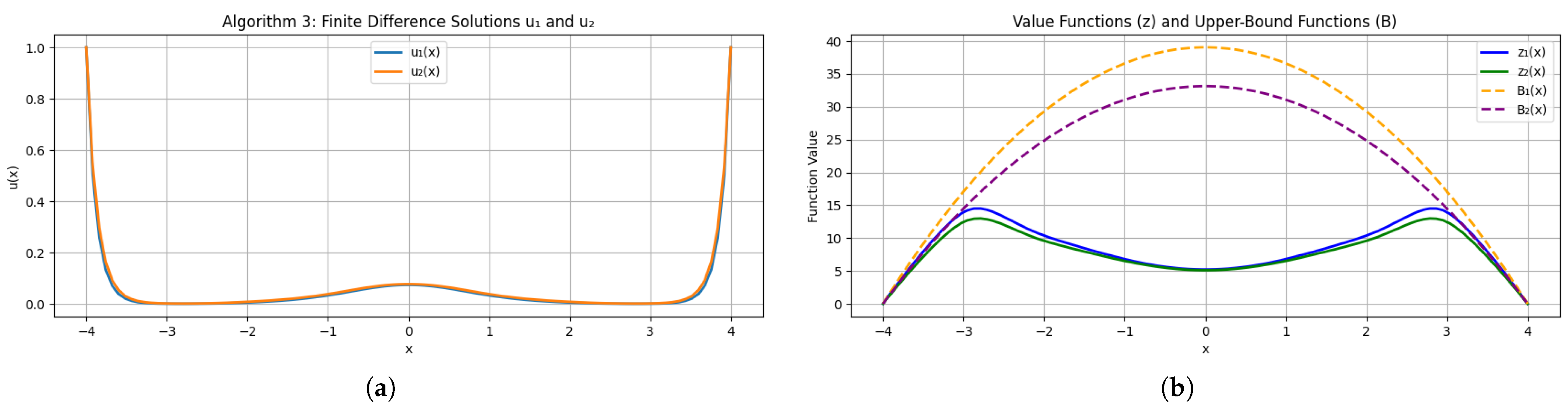
5.3.5. Case Study: Holding Cost Variation (Theorem 5)

To validate Theorem 5, we adopt parameters for a flexible manufacturing system [9] (

Table 4. Parameter set for Theorem 5 experiment.

Parameter	Regime 1	Regime 2	Interpretation
$a_i$	$0.6$	$0.9$	Transition rates
${\alpha }_i$	$0.3$	$0.3$	Common discount factor
$M_i$	5	4	Bounds on $f_i\left(x\right)$
${\sigma }_i$	1	1	Common volatility
$f_i\left(x\right)$	$5x^2$	$4x^2$	Regime-dependent cost
Domain	$x\in {\overline{B}}_4$		Boundary $R=4$

).

Figure 6a,b show the transformed solutions and value functions, demonstrating $z_1\ge z_2$ as $f_1>f_2$.

Next, we characterize the time evolution of the optimal production rate and inventory level under varying holding cost regimes (Figure 7).

Interpretation

The steeper penalty in regime 1 elevates $z_1$ over $z_2$, in full agreement with Theorem 5. These parameters model a production environment where the drift coefficients $a_i$ and switching intensities ${\alpha }_i$ reflect dynamic operational regimes, while $M_i$ and ${\sigma }_i$ capture the production capacities and uncertainties inherent in the system. The quadratic cost functions $f_1$ and $f_2$ impose steeper penalties for deviations in production levels, thereby promoting a robust control strategy.

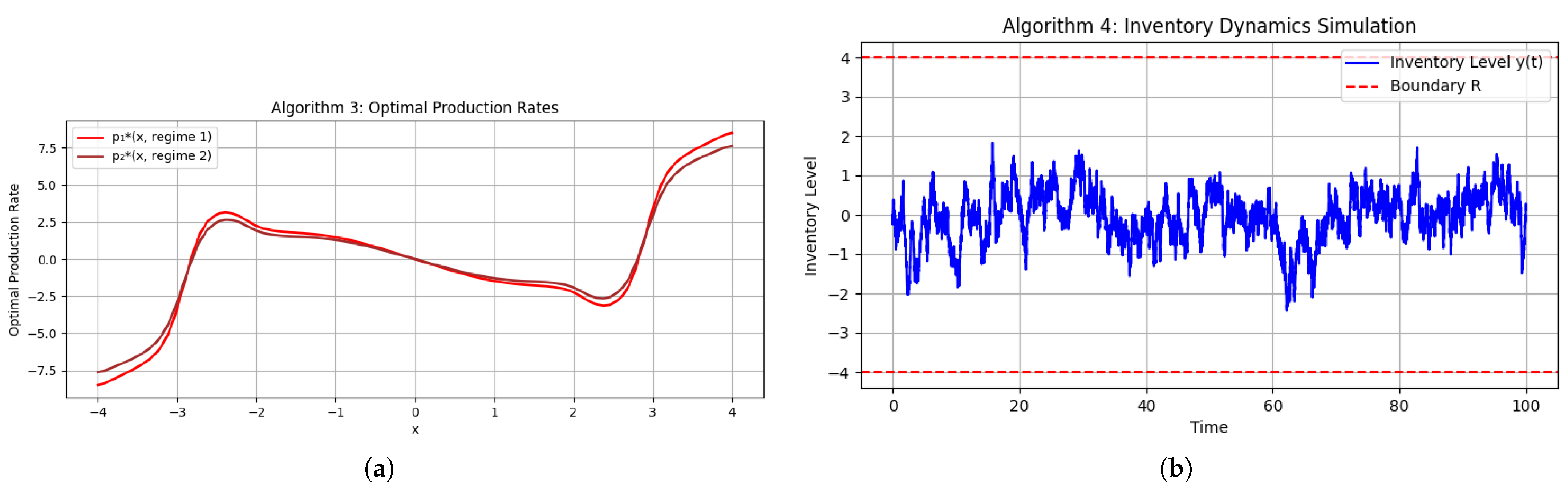
5.3.6. Case Study 4: Automotive Manufacturing (Theorem 6)

We adopt a parameter set inspired by modern automotive production, “e.g., companies like Dacia from România” where planning must react to volatile demand and supply chain risks.

This case study shows how to choose and interpret each model parameter in practice and how the two regimes arise in an automotive production context (e.g., Dacia Logan at Mioveni România).

Parameter Forms and Existence Conditions

To invoke Theorem 6, we must ensure

$$f_i\left(x\right)=M_i{\parallel x\parallel }^2,{\alpha }_i>0,{\sigma }_i>0,a_i>0.$$

Here

• Quadratic holding cost: We model inventory holding costs by

  $$f_i\left(x\right)=M_i{\parallel x\parallel }^2.$$
  A quadratic form captures rising marginal costs (e.g., storage, insurance) and the scalar $M_i$ bounds the curvature.
• Positive discount rates: ${\alpha }_i>0$ assures that future costs are appropriately down-weighted, guaranteeing a finite-value function.
• Non-degenerate volatility:${\sigma }_i>0$ models random demand or supply chain shocks in regime i.
• Irreducible regimes:$a_i>0$ are the Markov chain transition intensities, so each state recurs on average in $1/a_i$ time units.

Regime Interpretation

We assume two operational regimes driven by market and supply chain conditions:

• Regime 1 (High Demand) $a_1=0.6$: On average 1.7 months until demand cools; ${\sigma }_1=1.0$: large volatility from rush orders; ${\alpha }_1=0.3$: lower discounting of near-term costs; $M_1=5$: steep holding cost penalty to curb overstocking.
• Regime 2 (Low Demand) $a_2=0.9$: On average 1.1 months until demand rebounds; ${\sigma }_2=0.3$: stable production; ${\alpha }_2=0.8$: higher discounting of distant costs; $M_2=1$: mild inventory penalty to maintain minimal safety stock.

Interpreting the Transition Rate $a_1=0.6$

In our two-state Markov model, the time spent in regime 1 (high demand) is exponentially distributed with rate parameter $a_1$. By standard properties of the exponential law, the expected sojourn time in regime 1 is

$$\mathbb{E}\left[{\tau }_1\right]={\displaystyle \frac{1}{a_1}}={\displaystyle \frac{1}{0.6}}\approx 1.67\mathrm{months}.$$

Thus, once the system enters the high-demand regime, it will, on average, remain there for about $1.7$ months before switching back to the low-demand regime. This interpretation allows practitioners to translate the abstract rate $a_1$ directly into a familiar planning horizon—about seven weeks of sustained peak conditions under regime 1.

Table 5. Parameters for Theorem 6 experiment.

Parameter	Regime 1 (High)	Regime 2 (Low)
Transition rate $a_i$	$0.6$	$0.9$
Discount ${\alpha }_i$	$0.3$	$0.8$
Holding cost bound $M_i$	5	1
Volatility ${\sigma }_i$	$1.0$	$0.3$
Holding cost $f_i\left(x\right)$	${5\parallel x\parallel }^2$	${\parallel x\parallel }^2$
Inventory capacity R	4 units

displays the concrete numbers.

Numerical Implementation

• Solve the transformed PDE system (5) on the ball $\{\parallel y\parallel \le R\}$ by monotone Picard iteration, initializing with the super solution $u_i^{\left(0\right)}\left(y\right)=1$.
• Back-transform to obtain the following value functions:

  $$z_i\left(y\right)=-{\displaystyle \frac{2}{{\sigma }_i^2}}{K}_{i}ln{u}_i\left(y\right),i=1,2,$$

  where $K_i<0$ are the unique roots from Lemma 1.
• Compute the feedback control

  $$p_i^{*}(y,j)=-\frac{1}{2}{\partial }_{y_i}{z}_j\left(y\right),j\in \{1,2\}.$$
• (Optional) Validate by simulating $N=1000$ Euler–Maruyama paths of

  $$dy\left(t\right)=p^{*}(y\left(t\right),\epsilon \left(t\right))dt+{\sigma }_{\epsilon \left(t\right)}dW\left(t\right)$$

  until $\parallel y\parallel \ge R$.

Convergence and Interpretation

Executing the Python script in Appendix A.3 yields the following figures.

Figure 8 and Figure 9 demonstrate the following:

• Rapid, uniform convergence of $(u_i,z_i)$ at all grid nodes, as predicted by Theorem 6.
• Regime-tailored controls: During high demand (${\sigma }_1$ large; ${\alpha }_1$ small), the policy pre-emptively ramps production; during low demand, it throttles output to preserve cash.
• Theoretical bounds: The computed $z_i$ lie strictly between the bounded limits that underlie the existence of a proof.

By following this parameter selection recipe and interpreting each $a_i$, ${\alpha }_i$, $M_i$, and ${\sigma }_i$ in business terms, we consider that any practitioner can instantiate Theorems 3–6 for their own two-regime production inventory problem.

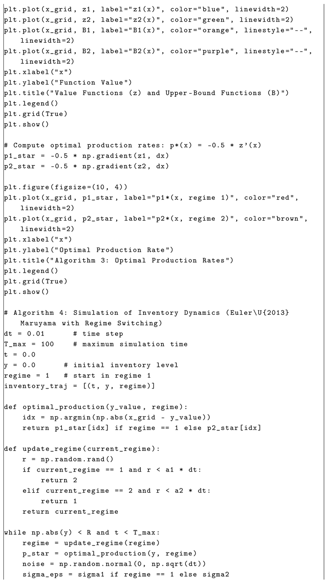
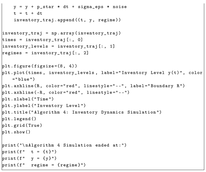
5.3.7. Implementation Notes

The full Python code (Appendix A.3) is annotated step by step: each function call is commented to clarify mesh setup, PDE discretization, monotone iteration, and post-processing. For the above examples, the annotated Python routine prints the nonlinear solver settings and the convergence statistics compiled in

Table 6. Nonlinear solver constants and convergence metrics for the four case studies (Theorems 3–6).

Thm.	Parameter Variation	${\mathit{K}}_1$	${\mathit{K}}_2$	${\mathsf{\Lambda }}_1$	${\mathsf{\Lambda }}_2$	Picard Its.
3	Volatility: ${\sigma }_1>{\sigma }_2$	$-0.71$	$-14.51$	$-27.93$	$-10,541.99$	1237
4	Discount rate: ${\alpha }_1<{\alpha }_2$	$-0.66$	$-1.08$	$-35.28$	$-37.38$	448
5	Holding cost: $f_1\left(x\right)>f_2\left(x\right)$	$-1.21$	$-1.03$	$-85.89$	$-69.72$	1097
6	Combined limits	$-1.22$	$-0.45$	$-85.89$	$-42.54$	1176

.

The negative $K_i$ and ${\Lambda }_i$ guarantee convexity and damping in the transformed PDEs, while rapid global convergence confirms the method’s suitability for real-time production planning under uncertainty.

5.3.8. Discussion and Practical Insights

Across all four experiments, the empirical ordering of $z_1\ge z_2$ agree with our theorems; this convergence demonstrates robustness, and in automotive production planning, rapidly changing regimes (peak/off peak, supply shocks) can be managed by our regime-switching feedback law $p^{*}\left(y\right)$, ensuring inventory targets are met with minimal cost.

Future work should extend to non-quadratic costs, correlated Brownian motions (see [12], for the resulting system), and higher-dimensional product portfolios.

Remark 1.

It is important to highlight that specific parameters require algorithmic application, each with an associated margin of error. In all the above considered scenarios, our theoretical results establish that

$$z_1\left(x\right)\le B_1\left(x\right)and{z}_2\left(x\right)\le B_2\left(x\right),forallx\in {\overline{B}}_R,$$

(11)

where the inequalities serve as a foundational guideline. In cases where these conditions are violated, the initial data must undergo adjustments to ensure the value functions align with (11). With the parameters explicitly defined, updating the Python code becomes easier; we only need to adjust these values directly when model parameters change, rather than re-running iterative numerical solvers.

6. Some Future Directions

Building on our stochastic production planning framework with regime-switching, we outline four concise avenues for future work:

• Alternative Convex Loss Functions. Replace the quadratic cost functional by other convex penalties (e.g., logarithmic or exponential) to better reflect industry-specific cost structures. Such non-quadratic losses introduce nonlinear terms into the HJB system, calling for novel analytical approximations or specialized numerical schemes.
• Correlated Brownian Motions. Allow nonzero correlations among the Brownian drivers to model interdependencies across product demands. The ensuing mixed-derivative terms in the coupled PDEs increase both theoretical complexity and computational burden, and yield a richer and more realistic description of cross-good risk.
• Geometric Inventory Dynamics. Model inventory levels via geometric Brownian motion to enforce non-negativity. The multiplicative noise and drift require a logarithmic change of variables and adaptive discretization (e.g., mesh refinement or implicit solvers) to maintain stability and accuracy.
• Real-Time Regime Detection. Integrate machine learning techniques (e.g., online change point detection, hidden Markov model inference) to identify economic regime shifts on the fly. Coupling an ML-based detector with the control law promises faster adaptation and enhanced robustness to structural breaks.

7. Conclusions

The production planning problem is solved using a value function approach, where the optimal production policy is characterized by a system of elliptic PDEs. This paper aims to bridge the gap between theoretical modeling and practical implementation, providing robust tools for stochastic production planning under regime-switching parameters. The regime-switching framework provides actionable insights for managerial decision-making, policy analysis, and operational optimization.

The contributions of this study include a derivation of the Hamilton–Jacobi–Bellman (HJB) equations and their transformation into an elliptic PDE system; the development of a monotone iteration scheme to approximate solutions, enabling quantitative analysis of production policies; an investigation of the impacts of volatility, holding costs, and discount rates on the value functions; and a comparison of models with and without regime-switching, highlighting the conservative and balanced predictions of regime-switching models.

By adapting production strategies to economic cycles, minimizing costs, and mitigating risks, the model enhances practical applicability in industries such as automotive manufacturing, energy systems, and retail.