Abstract
This paper analyzes the stability of trajectory tracking in fixed-wing UAV swarms subject to time-delayed feedback control. A delay-dependent stability criterion is established using a combination of Routh–Hurwitz analysis and a transcendental characteristic equation method. The study identifies a critical delay threshold beyond which the tracking objective becomes unstable. The influence of delayed feedback on the system dynamics is analyzed, showing how time delays affect the swarm’s ability to maintain formation. Numerical simulations confirm the theoretical predictions and illustrate the loss of stability as the delay increases. The findings underline the importance of accounting for delays when evaluating control performance in UAV swarm coordination.
MSC:
34K20; 93D30; 93B18
1. Introduction
Coordinated control of UAV (unmanned aerial vehicle) swarms has become a fundamental challenge in distributed systems, especially under time-delayed feedback caused by communication or computation constraints. Fixed-wing UAVs, in particular, offer advantages in endurance and range, making them suitable for applications in environmental monitoring, reconnaissance, and surveillance. However, their nonlinear dynamics and strict kinematic constraints introduce sensitivity to feedback delay, which can critically affect formation tracking and system stability.
Early contributions in multi-agent coordination laid the theoretical foundation for distributed consensus algorithms. Studies in [1,2] addressed consensus dynamics for single- and double-integrator systems, which were later extended to distributed vehicle coordination frameworks [3,4]. In the context of UAVs, specific challenges for fixed-wing models—including aerodynamic constraints—have been well documented [5].
Classical control strategies use Lyapunov–Krasovskii functionals [6] and convex optimization-based techniques such as reciprocally convex inequalities [7], along with frequency-domain criteria [8], to derive delay-dependent stability conditions. These methods are essential in deriving robust conditions but may become overly conservative or complex when applied to nonlinear systems. More recent studies include formation control of fixed-wing UAVs under communication delays using Lyapunov–Krasovskii functionals and leader–follower structures [9], event-triggered strategies for networked systems with delay and uncertainty compensation [10], and observer-based feedback stabilization [11,12], with increasing relevance for UAV swarms operating under network-induced latency.
The integration of data-driven and hybrid methods has broadened the range of available tools for time-delay modeling. A sparse identification framework for discovering delay differential systems from time series has been proposed in [13], while numerical solvers for mixed neutral-type equations were advanced in [14]. In aerospace applications, LSTM-based predictive architectures have been employed to mitigate feedback latency in aerodynamic systems [15]. Additionally, event-triggered stabilization for uncertain cyber–physical systems with time delay was investigated using Lyapunov-based co-design in [16]. In parallel, theoretical models have demonstrated that discrete delays can induce oscillations and bifurcations even in simple ecological or competition dynamics [17], underlining the importance of accurate stability boundaries.
Despite the extensive efforts in both theoretical analysis and control design for delay systems, few studies provide analytical tools that can explicitly determine stability limits in nonlinear UAV formations. Many existing methods rely on numerical simulations or approximations that do not yield closed-form conditions. This paper aims to fill this gap by developing a delay-dependent analytical approach applicable to fixed-wing UAV swarms.
Main Contributions
This paper addresses the problem of delay-induced instability in fixed-wing UAV swarm trajectory tracking, under a nonlinear control law affected by constant communication delay. The main contributions are as follows:
- A nonlinear tracking control law with constant time-delayed state feedback is formulated for fixed-wing UAVs in a leader–follower configuration;
- The resulting dynamics are cast as a delay differential system, and a transcendental characteristic equation is derived;
- Stability conditions and critical delay thresholds are computed using a hybrid Routh–Hurwitz and Cooke–van den Driessche analytical framework;
- The influence of control parameters on the delay margin is explored through a sensitivity analysis;
- The theoretical predictions are validated through numerical simulations using MATLAB’s DDE solvers.
The proposed methodology complements hierarchical [18] and learning-based strategies [15] by providing explicit analytical margins for stability, particularly important in time-critical missions involving fixed-wing UAV swarms.
2. The Mathematical Model
We analyze the scenario in which all vehicles maintain a constant altitude. As in [12,18], we introduce the system that describes the motion of a fixed-wing UAV in 2D:
where represents the mass center in the inertial frame, and is the heading angle of UAV i with respect to the x axis. The control inputs are given by the forward speed and the angular speed . Consider a leader vehicle modeled by Equation (1), with its position represented by , heading angle , forward speed , and heading rate by (see [18]). The problem addressed in [18], as well as in many other studies, is to find a control law for UAV i modeled by Equation (1) in the form of
where is a smooth function, such that
where is the desired relative position of UAV i with respect to vehicle 0, the leader. Using a coordinate transformation in the UAV’s body frame, we obtain the following:
From this, it follows that in order to achieve the objective represented by Equation (2), it suffices to show that, for all initial states and , the following conditions hold:
From Equation (1) and the transformation in Equation (3), the motion of the UAV is described as follows:
The control laws for the UAV are given as follows:
where the notation is used. For convenience, we drop the index i in the following derivations.
To simplify the analysis and improve the clarity of the model, we define the following auxiliary functions, which represent the nonlinear, delay-dependent control terms:
The delay-affected feedback terms and modulate the control inputs based on past state information. Their contribution to the system Jacobian changes with the delay, directly influencing the location of characteristic roots and therefore the stability properties of the closed-loop dynamics.
Using this notation, the system dynamics can be rewritten in a compact form:
We now analyze the local behavior of the nonlinear functions introduced above, in the neighborhood of the equilibrium point.
Lemma 1.
Assume that . Then, the auxiliary functions satisfy the following:
Hence, both and are smooth near the origin and can be linearized for the purpose of stability analysis.
Proof.
A first-order Taylor expansion around zero gives
Substituting in the expression of and keeping only linear terms completes the proof. □
To establish the stability of the tracking trajectory, it is necessary to prove the asymptotic stability of the zero equilibrium of system (7). To achieve this, we consider the matrices A and B, which represent the components of the Jacobian matrix of system (7) evaluated at the equilibrium point:
The characteristic equation associated with the system takes the following form:
For further analysis, we introduce the following notations:
The Routh–Hurwitz stability criterion provides the following conditions:
Proposition 1.
Equation (10) is stable for .
Proof.
To establish stability, it is sufficient to verify that the following conditions hold:
□
Next, we introduce the following notations:
Starting from the characteristic Equation (10), and using the notation from (11) and (13), it can be expressed as follows: (10) can be rewritten as
Using a standard approach, we seek solutions with zero real parts, identifying cases where eigenvalues cross the imaginary axis from left to right.
Recalling from [19], we state the following theorem, adapted to our problem:
Theorem 1.
Assume that are independent of τ and satisfy the following conditions:
(i) and have no common imaginary zero.
(ii) Each are polynomials with real coefficients.
(iii)
(iv) The degree of is greater than the degree of
Following [19], we define
and
Then,
- (a)
- Suppose that the equation has no positive roots. Then, if (14) is stable at , it remains stable for all , whereas if it is unstable at , it remains unstable for all .
- (b)
- Suppose that the equation has at least one positive real root and that each positive root is simple. As τ increases, stability switches may occur. There exists a positive number such that Equation (14) is unstable for all . As τ varies from 0 to , at most a finite number of stability switches may occur.
Remark 1.
The derived criterion not only confirms the local stability for but also provides a mechanism to detect multiple stability switches as τ increases. This makes the method suitable for designing delay-tolerant controllers in networks with time-varying delays. Furthermore, the analytical expressions for allow identifying the direction of eigenvalue crossings and estimating robustness margins.
We combine classical Routh–Hurwitz conditions for the no-delay case with a transcendental stability approach based on the method of Cooke and van den Driessche. The characteristic equation is expressed in exponential–polynomial form and analyzed for critical roots crossing the imaginary axis.
By multiplying using Equation (14) with , we obtain an equivalent equation in the following form:
To follow the considerations that led to Proposition 1 from [19], consider a root of Equation (15), so
Then, such a root will also satisfy . From (16), we obtain
In order to solve this system with respect to and , we introduce
Since
we obtain the following equation:
Thus, Equation (18) can be rewritten in its extended form as follows:
The solutions of the above equation determine the values of μ that satisfy Equation (16). Then, the corresponding values of are given as follows:
These values represent the points where stability switches might occur. To determine whether this is the case, we compute the sign of the real part of at and , as in [19]:
where
Remark 2.
Unlike traditional methods based on Lyapunov–Krasovskii functionals or LMI techniques, our approach provides explicit delay thresholds derived from the roots of a transcendental characteristic equation. This enables analytical identification of stability switches and is particularly useful in systems with high sensitivity to delay, such as fixed-wing UAVs operating in tightly coupled formations. Furthermore, in contrast to the hierarchical coordination methods in [18], our method is delay-centric and suitable for evaluating robustness margins analytically.
The theoretical analysis provides conditions for system stability and identifies potential stability switches depending on the delay parameter τ. To further validate these findings, numerical computations and simulations were performed to observe the system’s behavior under different parameter settings. The simulations illustrate how the system evolves over time and verify whether the theoretical predictions hold in practice.
3. Numerical Results and Simulations
The parameters used for numerical calculations, as referenced in the cited sources, are summarized in Table 1:

Table 1.
Parameter values used in the numerical simulations.
All simulations were conducted in MATLAB 2024 using the built-in dde23 solver. A fixed integration time step of s was used to ensure numerical stability and precision.
With these values, one solution of Equation (18) is , which gives . Following the calculations for the expression (20), the result has a positive sign, indicating that stability is lost when the delay exceeds the threshold .
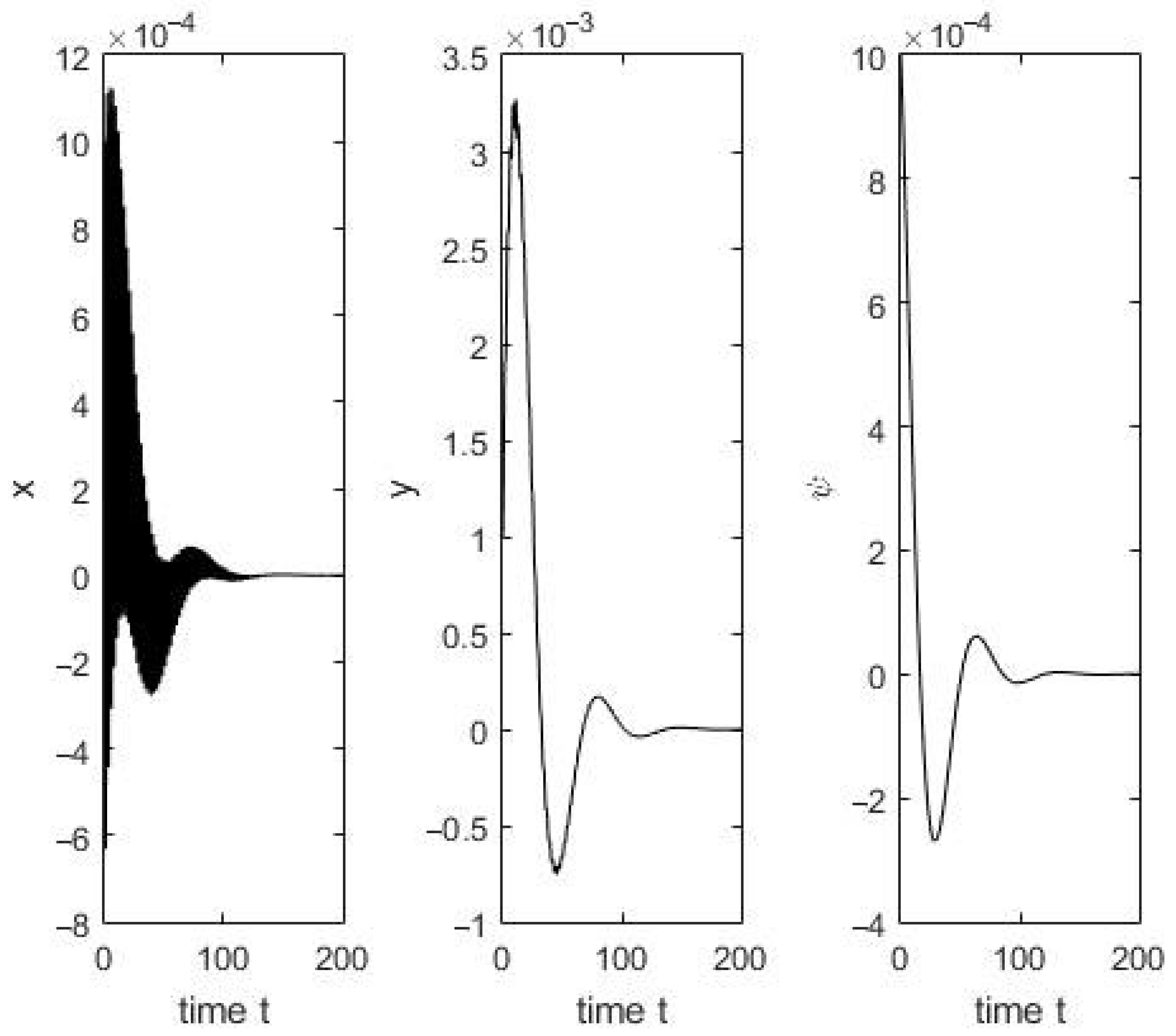
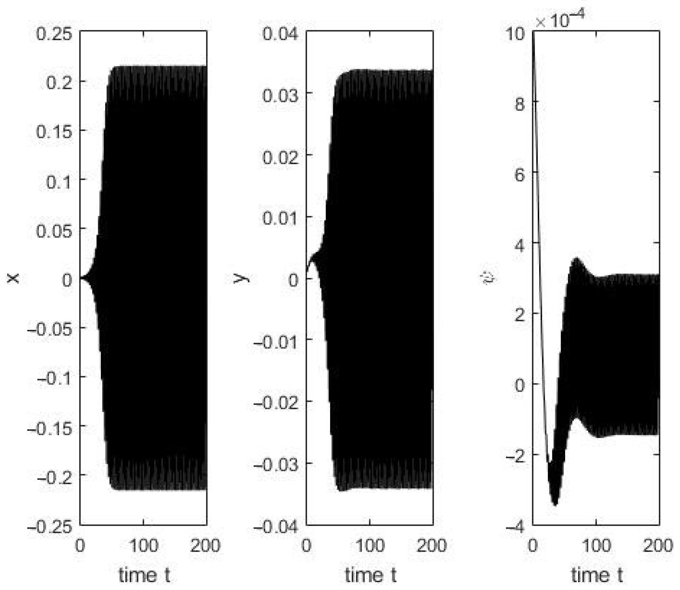
As the delay approaches or exceeds the critical value , the system’s ability to accurately follow the reference trajectory degrades significantly. This manifests as persistent tracking error and growing oscillations, in contrast to the stable response with fast convergence shown in Figure 1 for , and as seen in Figure 2.

Figure 1.
Stable system with fast convergence, .
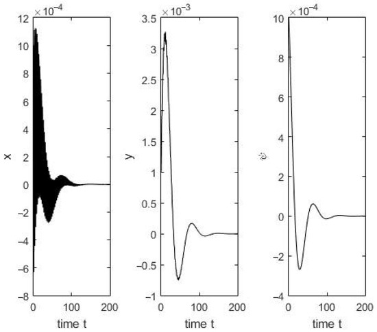
Figure 2.
Transition to instability, .
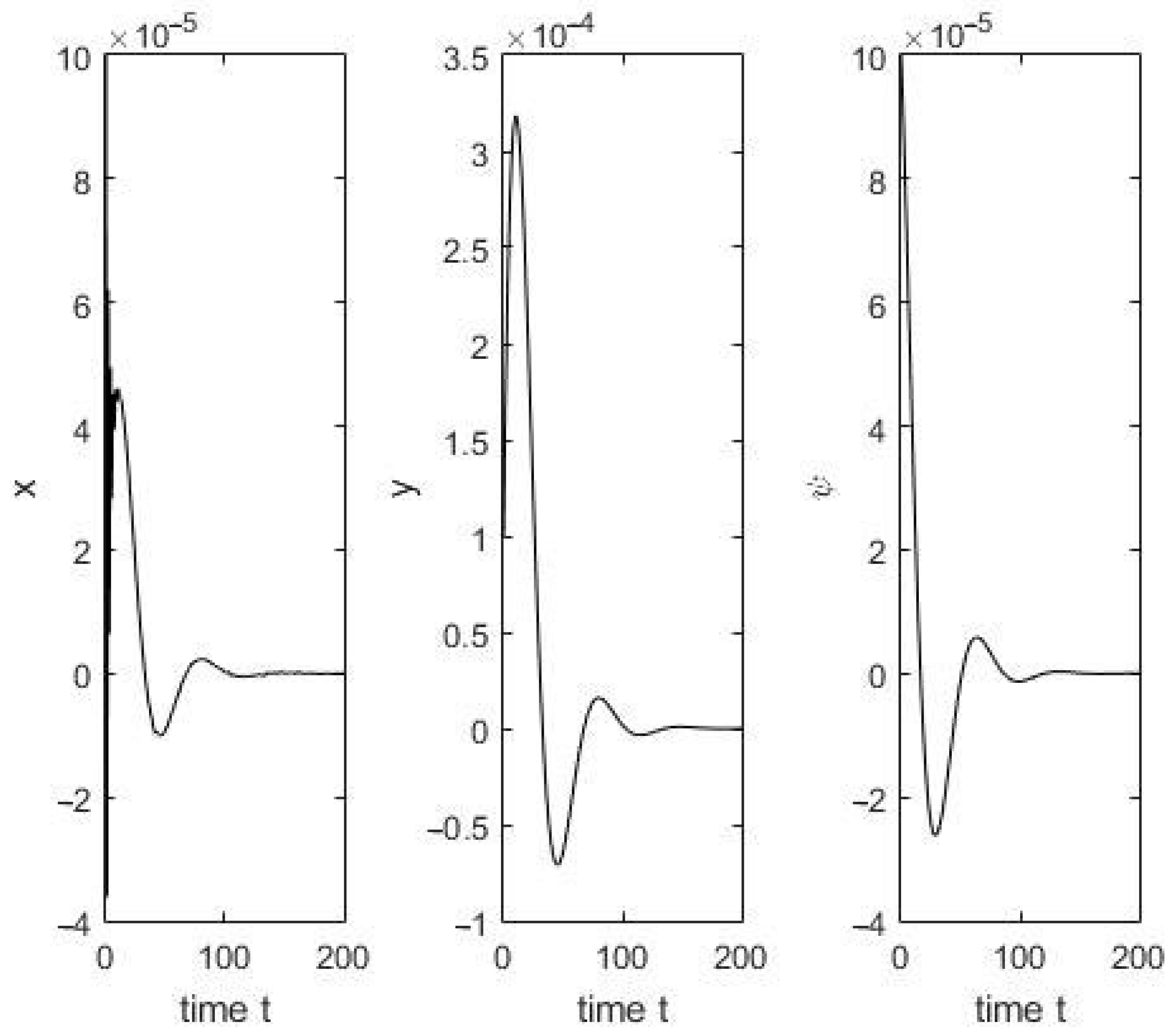
To further validate the theoretical findings, we first analyze the system’s response for delays close to and beyond the critical threshold. As shown in Figure 3, when , strong oscillations emerge, clearly indicating instability. This behavior becomes even more pronounced in Figure 4, where the system becomes fully unstable for .
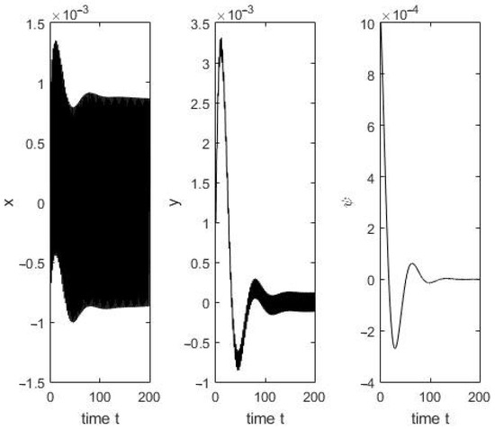
Figure 3.
Strong oscillations indicating instability, .

Figure 4.
Fully unstable system, .
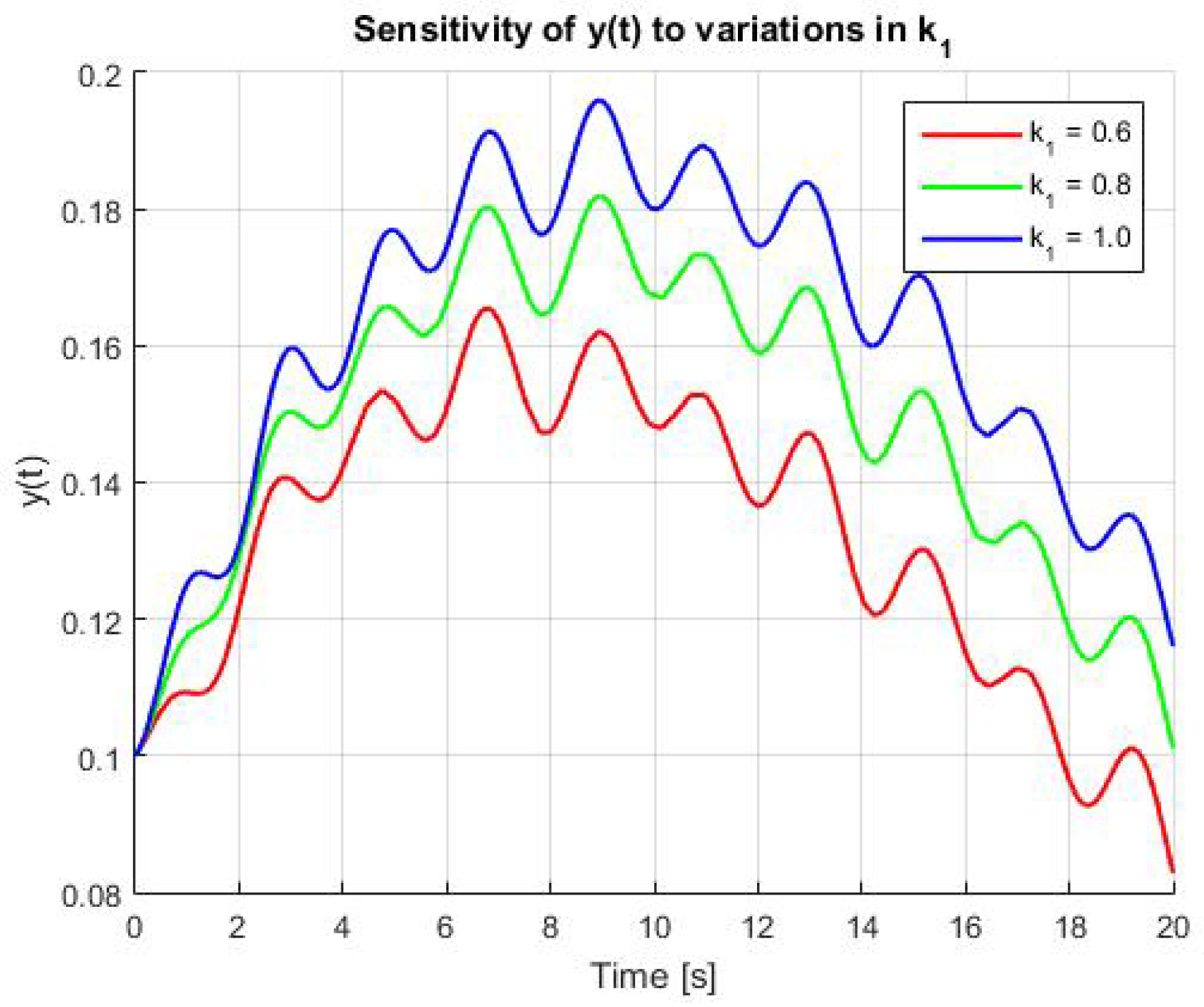
To complement the theoretical results, we performed a time-domain simulation using the delayed model under varying values of the control parameter , while keeping the delay fixed below the critical threshold (). The results, shown in Figure 5, illustrate that increasing leads to more pronounced oscillations in the y-component of the trajectory.
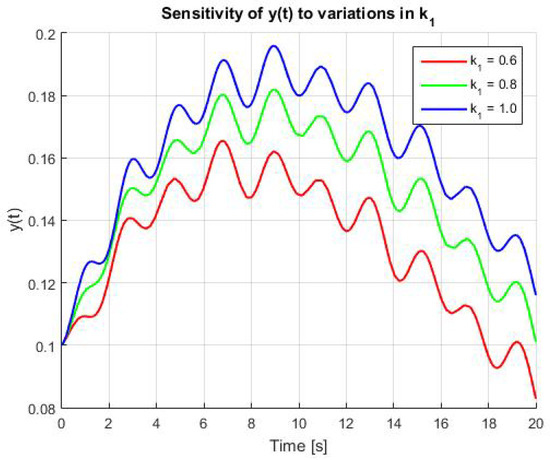
Figure 5.
Evolution of for different values of , with fixed. As increases, the system becomes more sensitive to delay, exhibiting larger oscillations and slower decay.
From a practical perspective, the critical delay serves as a constraint in the design of real-world UAV swarm systems. In applications involving distributed control over communication networks, delays due to processing, transmission, or congestion must remain below this threshold to ensure stable trajectory tracking. This theoretical analysis thus provides a quantitative criterion for delay-aware control design.
This is consistent with the analytical prediction that the critical delay decreases as increases, confirming that more aggressive feedback can destabilize the system earlier in the presence of delay.
The simulations confirm the predicted critical delay threshold by showing that, for , the system remains stable, while for , it exhibits divergent or oscillatory behavior. Additional sensitivity simulations support the delay dependence of tracking performance.
4. Conclusions
The model introduced in [18] was modified to include control delays, which may result from communication issues. The analysis identified critical delay thresholds beyond which the tracking trajectory becomes unstable. These thresholds were derived using linear stability analysis and the characteristic equation of the system.
Numerical computations and simulations confirmed that exceeding the theoretical delay limits leads to instability in trajectory tracking. The proposed control law was tested under various delay values, and the results demonstrated that the system remains robust within allowable delay bounds. Simulations also showed the impact of delays on tracking performance.
The findings highlight the importance of considering communication delays when designing control strategies for UAV swarms. This work provides a basis for developing delay-tolerant control methods and can be extended to more complex dynamic models in future research.
The current study focused on delay-induced instability under idealized, disturbance-free conditions. However, in practical UAV applications, external perturbations such as wind gusts or sensor noise may significantly affect system performance. A natural extension of this work is to include such disturbances in the model and analyze the robustness of the delay threshold using Lyapunov–Krasovskii or methods. This direction will be considered in future research.
Author Contributions
Conceptualization, A.H. and A.-M.B.; methodology, A.H. and A.-M.B.; software, A.-M.B.; validation, A.-M.B.; formal analysis, A.H. and A.-M.B.; investigation, A.-M.B.; writing—original draft preparation, A.-M.B.; writing—review and editing, A.-M.B.; visualization, A.-M.B.; supervision, A.H. All authors have read and agreed to the published version of the manuscript.
Funding
This research was supported by the Romanian Ministry of Research, Innovation and Digitalization: NUCLEU Program project code PN 23-17-06-03, Ctr. 36 N/12.01.2023.
Data Availability Statement
The original contributions presented in the study are included in the article, further inquiries can be directed to the corresponding authors.
Conflicts of Interest
The authors declare no conflicts of interest.
References
- Olfati-Saber, R.; Fax, J.A.; Murray, R.M. Consensus and cooperation in networked multi-agent systems. Proc. IEEE 2007, 95, 215–233. [Google Scholar] [CrossRef]
- Jadbabaie, A.; Lin, J.; Morse, A.S. Coordination of groups of mobile autonomous agents using nearest neighbor rules. IEEE Trans. Autom. Control 2003, 48, 988–1001. [Google Scholar] [CrossRef]
- Michiels, W.; Niculescu, S.-I. Stability and Stabilization of Time-Delay Systems: An Eigenvalue-Based Approach; SIAM: Philadelphia, PA, USA, 2007. [Google Scholar]
- Ren, W.; Beard, R.W. Distributed Consensus in Multi-Vehicle Cooperative Control: Theory and Applications; Springer: London, UK, 2008. [Google Scholar]
- Beard, R.W.; McLain, T.W. Small Unmanned Aircraft: Theory and Practice; Princeton University Press: Princeton, NJ, USA, 2012. [Google Scholar]
- Fridman, E.; Shaked, U. Delay-dependent stability and H∞ control: Constant and time-varying delays. Int. J. Control 2003, 76, 48–60. [Google Scholar] [CrossRef]
- Modala, T.; Patra, S.; Ray, G. An improved delay-dependent stabilization criterion of linear time-varying delay systems: An iterative method. Kybernetika 2023, 59, 633–654. [Google Scholar] [CrossRef]
- Gu, K.; Kharitonov, V.L.; Chen, J. Stability of Time-Delay Systems; Springer: Boston, MA, USA, 2003. [Google Scholar]
- Du, Z.; Qu, X.; Shi, J.; Lu, J. Formation control of fixed-wing UAVs with communication delay. ISA Trans. 2024, 146, 154–164. [Google Scholar] [CrossRef] [PubMed]
- Shen, Y.; Fei, M.; Du, D.; Peng, C.; Tian, Y.-C. Event-triggered robust H∞ control for uncertain networked control systems with time delay. Trans. Inst. Meas. Control 2020, 42, 284–297. [Google Scholar] [CrossRef]
- Saber, R.O.; Murray, R.M. Consensus protocols for networks of dynamic agents. Proc. Am. Control Conf. 2003, 2, 951–956. [Google Scholar]
- Yang, J.; Yin, D.; Shen, L. Reciprocal geometric conflict resolution on unmanned aerial vehicles by heading control. J. Guid. Control Dyn. 2017, 40, 2511–2523. [Google Scholar] [CrossRef]
- Pecile, A.; Demo, N.; Tezzele, M.; Rozza, G.; Breda, D. Data-driven discovery of delay differential equations with discrete delays. J. Comput. Appl. Math. 2025, 461, 116439. [Google Scholar] [CrossRef]
- Aggarwal, R.; Methi, G.; Agarwal, R.P.; Hussain, B. An efficient approach for mixed neutral delay differential equations. Computation 2025, 13, 50. [Google Scholar] [CrossRef]
- Li, L.; Xu, H.; Xing, Z.; Khan, A.S. Time-delay effect and design of closed-loop control system of circulation control airfoil. Chin. J. Aeronaut. 2024, 37, 50–67. [Google Scholar] [CrossRef]
- Du, Z.; Zhang, C.; Yang, X.; Ye, H.; Li, J. Discrete-time event-triggered H-infinity stabilization for three closed-loop cyber-physical systems with uncertain delay. Appl. Math. Comput. 2025, 488, 129127. [Google Scholar] [CrossRef]
- Wang, X.; Kottegoda, C.; Shan, C.; Huang, Q. Oscillations and coexistence generated by discrete delays in a two-species competition model. Discrete Contin. Dyn. Syst. Ser. B 2024, 29, 1798–1814. [Google Scholar] [CrossRef]
- Chen, H.; Wang, X.; Shen, L.; Cong, Y. Formation flight of fixed-wing UAV swarms: A group-based hierarchical approach. Chin. J. Aeronaut. 2021, 34, 504–515. [Google Scholar] [CrossRef]
- Cooke, K.; van den Driessche, P. On zeroes of some transcendental equations. Funkcialaj Ekvacioj 1986, 29, 77–90. [Google Scholar]

Disclaimer/Publisher’s Note: The statements, opinions and data contained in all publications are solely those of the individual author(s) and contributor(s) and not of MDPI and/or the editor(s). MDPI and/or the editor(s) disclaim responsibility for any injury to people or property resulting from any ideas, methods, instructions or products referred to in the content. |
© 2025 by the authors. Licensee MDPI, Basel, Switzerland. This article is an open access article distributed under the terms and conditions of the Creative Commons Attribution (CC BY) license (https://creativecommons.org/licenses/by/4.0/).