On the Conflation of Poisson and Logarithmic Distributions with Applications

Abstract

It is frequent for real-life count data to show inflation in lower values; however, most of the well-known count distributions cannot capture such a feature. The present paper introduces a new distribution for modeling inflated count data in small values based on a conflation of distributions approach. The new distribution inherits some properties from Poisson distribution (PD) and logarithmic distribution (LD), making it a powerful modeling tool. It can serve as an alternative to PD, LD, and zero-truncated distributions. The new distribution is worth considering theoretically, as it belongs to the weighted PD family. With zero as a support point, two additional models are suggested for the new distribution. These modifications yield distributions that demonstrate overdispersion models comparable to the negative binomial distribution (NBD) while retaining essential PD properties, making them suitable for accurately representing count data with frequent events of low frequency and high variance. Furthermore, we discuss the superior performance of three new distributions in modeling real count data compared to traditional count distributions such as PD and NBD, as well as other discrete distributions. This paper examines the key statistical properties of the proposed distributions. A comparison of the novel and other distributions in the literature is shown employing real-life data from some domains. All of the computations shown in this study are generated using the R programming language.

1. Introduction

The Poisson distribution (PD) is a fundamental discrete probability model commonly used to describe count data. It appears in a wide range of applications, including telecommunications, traffic engineering, biology, and insurance. One of its key characteristics is that the mean and variance are equal. However, this property limits its flexibility when the observed variance exceeds or falls below the mean, referred to as overdispersion and underdispersion, respectively, and then the PD may not provide a good fit.

Different generalizations have been suggested in the literature in order to expand the ability of PD in fitting a wide range of data, especially the overdispersed ones. The first type of generalization is to randomize the mean PD. The case where the mean follows the gamma distribution was considered by [1]. This resulted in a negative binomial distribution (NBD). Although a NBD can model overdispersion data, it has the restriction that variance is a quadratic function of the mean. Ref. [2] proposed Poisson Lindley distribution (PLiD) by assuming that the mean of PD follows the Lindley distribution. The PLiD is considered to be an approximation of the NBD and the Hermite distribution. Several authors have also suggested mixed Poisson distributions, such as the Poisson–Akash distribution (PAD) [3] and the Poisson–Shanker distribution (PSHD) [4].

The second approach to generalization involves introducing an additional parameter to a distribution to enhance its flexibility. For example, a study [5] presented a generalized Poisson distribution by replacing the PD parameter with a linear function of the count variable. Alternatively, ref. [6] introduced the Conway–Maxwell–Poisson distribution by increasing the probability mass function (pmf) of PD to a certain power, thus incorporating a new parameter.

The third technique to generalize PD includes using a weighting approach by multiplying count distributions with weight functions. The concept of weighted distributions was formulated in [7,8]. Weighted distributions offer a flexible framework that enables us to modify probabilities according to accurate weights assigned to each event, thus improving our capacity to accurately represent and evaluate challenging real-life phenomena. The flexibility of weighted distributions makes them useful in numerous domains; for additional information on this concept and its applications, review the study [9] on this particular subject.

Ref. [10] presented the concept of the conflation of probability distributions as a method to consolidate data from different independent experiments. For the case of two independent experiments, the conflation of the pmfs $f_1$ and $f_2$ denoted $f_C$ is defined by

$$f_C\left(x\right)={\displaystyle \frac{f_1\left(x\right)f_2\left(x\right)}{{\sum }_{y\in \psi }{f}_1\left(y\right)f_2\left(y\right)}},x\in \mathbf{N}.$$

(1)

where $\psi$ includes the common support points of the two distributions. Most of the examples in [10] are conflations of distributions belonging to the same family. Recently, ref. [11] introduced an original distribution based on conflating the NBD and the logarithmic distribution (LD), resulting in the conflation of a negative binomial-logarithmic distribution (CNBLD).

The CNBLD has advantageous statistical results and extensive applications, particularly in the areas of health and reliability theory. The CNBLD offers superior fitting compared to the NBD for count data with inflated lower counts. Nonetheless, the CNBLD exhibits a high dispersion similar to that of the NBD (see [11], Table 1), and hence, the CNBLD may be inadequate for modeling moderate dispersion. Consequently, this limitation motivates us to propose a new distribution with less dispersion compared to the CNBLD and increased dispersion relative to the PD. This distribution is a newly developed version of PD inherent to the concept of conflating probability distributions, which is the conflation of Poisson and logarithmic distributions (CPLD). The CPLD is characterized by a single parameter, which simplifies its use and interpretation and makes it suitable for various modeling applications. By integrating characteristics of the logarithmic and Poisson distributions, the flexibility of the CPLD goes beyond its parameterization. For example, it utilizes the fast decay of the pmf of LD to introduce a Poisson version with inflated low count. In addition, since LD supports only positive count, the CPLD enriches the class of positive count distributions. However, in order to use this distribution as an alternative to PD, we consider two modifications of CPLD that can model data with zero count. The first is to shift the CPLD one point to the left, resulting in a shifted CPLD that is denoted as SCPLD. The second modification is to conflate a shifted LD with the PD, yielding in the conflation of a Poisson shift logarithmic distribution (CPSLD).

The rest of the paper is as follows: In Section 2, we introduce the new models; Section 3 outlines some of the key statistical properties of the proposed models, such as moments, unimodality, dispersion index, and likelihood ratio stochastic order; Section 4 discusses the estimation of the parameters using the method of moments and the maximum likelihood method and assesses the estimates by a simulation study; Section 5 highlights the usefulness of the new distribution across several fields, showing its superior performance compared to the existing modified PD employed to fit similar data; finally, Section 6 presents a conclusion.

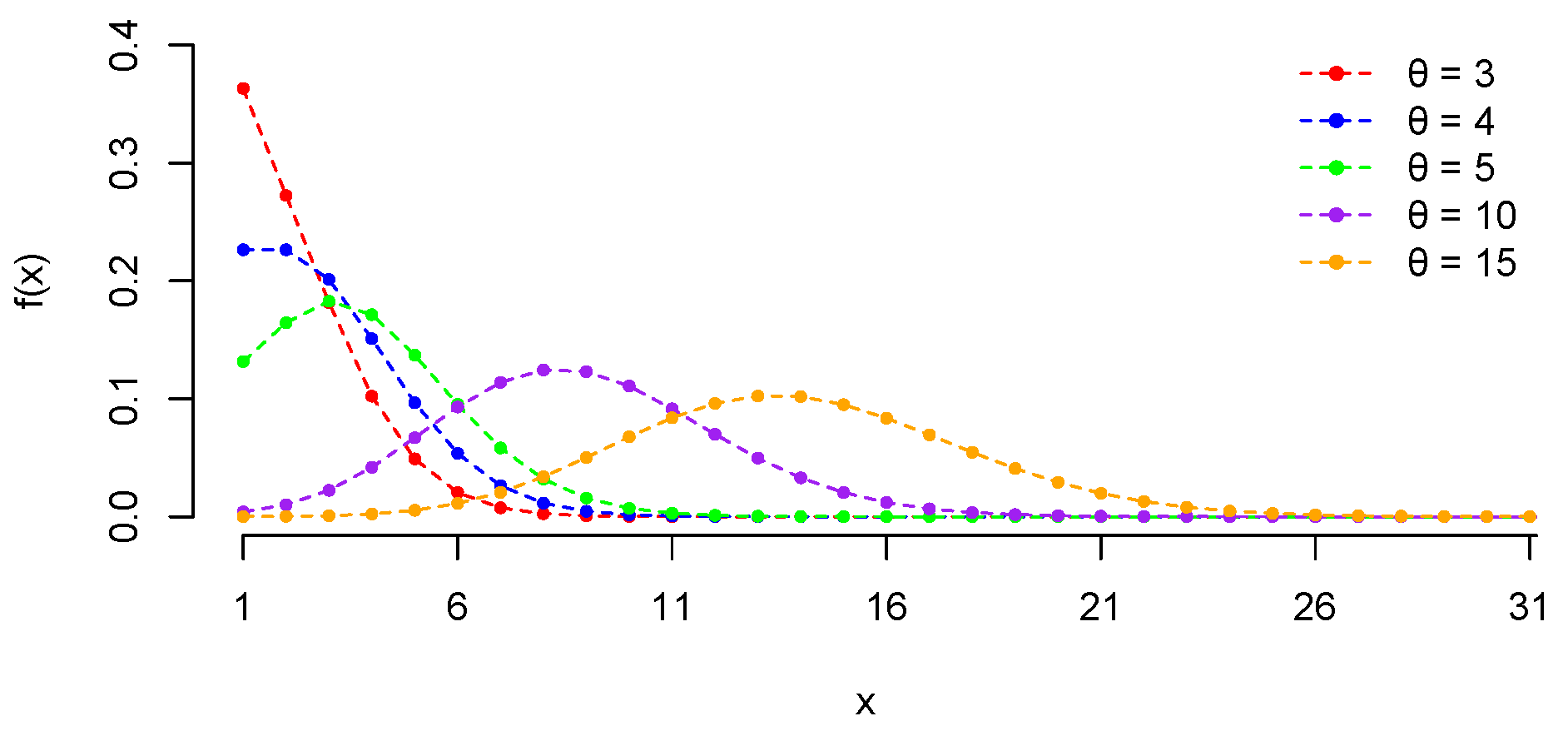
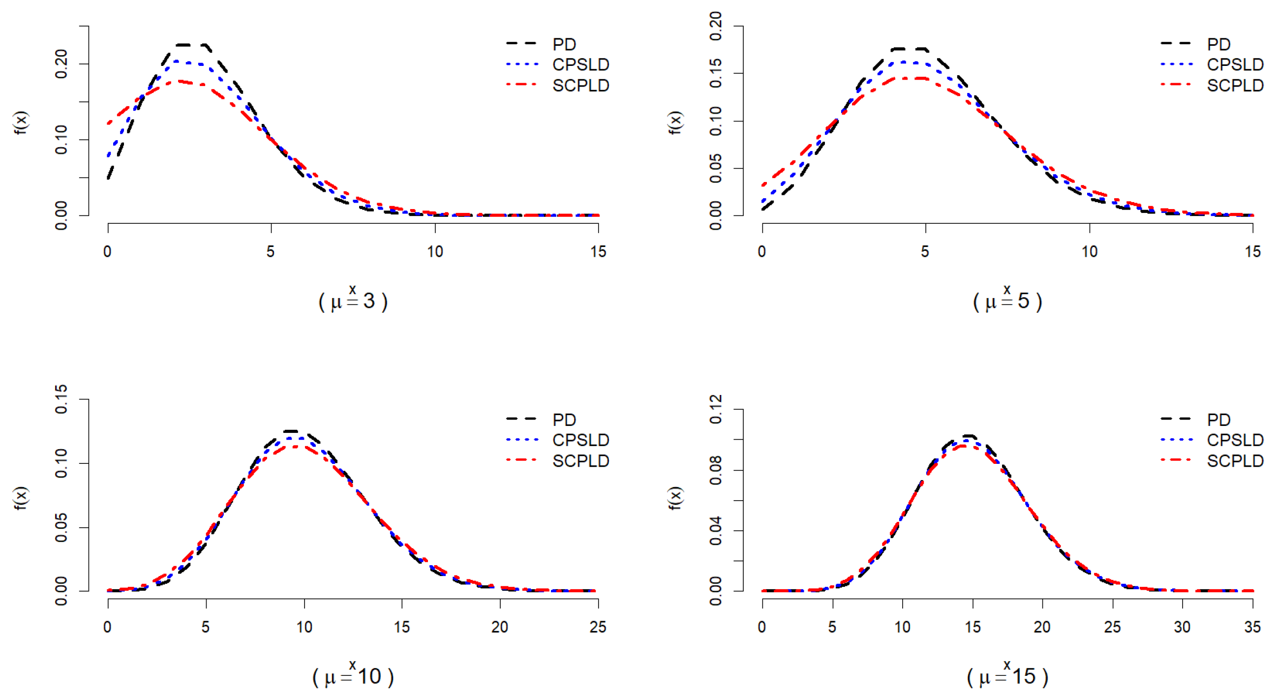
2. Conflated Poisson Logarithmic Distributions

This section introduces the conflated Poisson logarithmic distribution (CPLD) and its modifications, the SCPLD and the CPSLD. Here, we explore the probability mass functions pmfs, the cumulative distribution functions ($cdf$), represented as $F(·)$, the survival functions ($sf$), also indicated as ($\overline{F}(·)$), and the hazard rate functions (h) of the CPLD, SCPLD, and CPSLD. Equation (1) allows us to define the conflation of the Poisson and logarithmic distribution (CPLD) as follows:

$$f\left(x\right)={\displaystyle \frac{{\theta }^x}{C\left(\theta \right)xx!}},x=1,2,\dots .$$

(2)

where $C\left(\theta \right)={\sum }_{l=1}^{\infty }{\displaystyle \frac{{\theta }^l}{ll!}}$ and $\theta >0$. $C\left(\theta \right)$ is related to the exponential integral function defined by

$$\begin{array}{cc}\hfill Ei\left(\alpha \right)& ={\int }_{-\infty }^{\alpha }{\displaystyle \frac{e^t}{t}}dt\hfill \\ \hfill & =\gamma +ln\left(\alpha \right)+C\left(\alpha \right)\hfill \end{array}$$

where $\gamma =0.57721$ is the Euler–Mascheroni constant. For more details about $Ei(·)$, see [12].

The $cdf$, $sf$, and h of the CPLD are calculated using Gauss’s hypergeometric function, which is defined by

$${}_{2}F_2(a,b;c,d;\theta )=\sum _{n=0}^{\infty }{\displaystyle \frac{{\left(a\right)}_n{\left(b\right)}_n}{{\left(c\right)}_n{\left(d\right)}_n}}{\displaystyle \frac{{\theta }^n}{n!}}$$

where ${\left(a\right)}_n={\displaystyle \frac{\mathrm{\Gamma }(a+n)}{\mathrm{\Gamma }\left(a\right)}}$ is the Pochhammer symbol. See [9] for more details about the generalized hypergeometric function.

We start by calculation the $sf$ of CPLD as follows:

$$\begin{array}{cc}\hfill \overline{F}\left(x\right)& =\sum _{r=x+1}^{\infty }{\displaystyle \frac{{\theta }^r}{C\left(\theta \right)rr!}}\hfill \\ \hfill & ={\displaystyle \frac{A\left(x\right)}{C\left(\theta \right)rr!}}\hfill \end{array}$$

where

$$\begin{array}{cc}\hfill A\left(x\right)& =\sum _{r=x+1}^{\infty }{\displaystyle \frac{{\theta }^r}{rr!}}\hfill \\ \hfill & =\sum _{z=0}^{\infty }{\displaystyle \frac{{\theta }^{z+x+1}}{(z+x+1)(z+x+1)!}}\hfill \\ \hfill & ={\displaystyle \frac{{\theta }^{x+1}}{(x+1)(x+1)!}}\sum _{z=0}^{\infty }{\displaystyle \frac{z!(x+1)!(x+1)!(z+x)!}{x!(z+x+1)!(z+x+1)!}}{\displaystyle \frac{{\theta }^z}{z!}}\hfill \\ \hfill & ={\displaystyle \frac{{\theta }^{x+1}}{(x+1)(x+1)!}}\sum _{z=0}^{\infty }{\displaystyle \frac{{\left(1\right)}_z{(x+1)}_z}{{(x+2)}_z{(x+2)}_z}}{\displaystyle \frac{{\theta }^z}{z!}}\hfill \\ \hfill & ={\displaystyle \frac{{}_{2}F_2(1,x+1;x+2,x+2;\theta ){\theta }^{x+1}}{(x+1)(x+1)!}}.\hfill \end{array}$$

Then, the $sf$ can be written as

$$\overline{F}\left(x\right)={\displaystyle \frac{{}_{2}F_2(1,x+1;x+2,x+2;\theta ){\theta }^{x+1}}{C\left(\theta \right)(x+1)(x+1)!}}.$$

Here, the $cdf$ is given as

$$\begin{array}{cc}\hfill F\left(x\right)& =1-\overline{F}\left(x\right)\hfill \\ \hfill & =1-{\displaystyle \frac{{}_{2}F_2(1,x+1;x+2,x+2;\theta ){\theta }^{x+1}}{C\left(\theta \right)(x+1)(x+1)!}}\hfill \end{array}$$

and the h of the CPLD is

$$\begin{array}{cc}\hfill h\left(x\right)& ={\displaystyle \frac{{(x+1)}^2}{x\theta {}_{2}F_2(1,x+1;x+2,x+2;\theta )}},x=1,2,...\hfill \end{array}$$

In this study, the CPLD is extended by two approaches to accommodate distributions that yield zero value, which is necessary for the majority of applications. One method is to move the CPLD to the left by one position. In the second method, the shifted logarithmic distribution is employed instead of the LD. Hence, below are the two definitions that follow.

Definition 1.

The random variable X is said to follow the shifted conflation of Poisson logarithmic distributions (SCPLD) with parameter $\theta >0$ if its pmf is given by

$$f_{\mathrm{SCPLD}}\left(x\right)={\displaystyle \frac{{\theta }^{x+1}}{C\left(\theta \right)(x+1)(x+1)!}},x=0,1,2,\dots .$$

Definition 2.

The random variable X is said to follow the conflation of Poisson shifted logarithmic distribution (CPSLD) with parameter $\theta >0$ if its pmf is given by

$$f_{\mathrm{CPSLD}}\left(x\right)={\displaystyle \frac{{\theta }^{x+1}}{(e^{\theta }-1)(x+1)!}},x=0,1,2,\dots .$$

Remark 1.

The CPSLD can be interpreted as a shifted zero-truncated PD.

Next, we study the shape of the pmfs of the CPLD for different values of $\theta$. Figure 1 exhibits the plots for $\theta =3,4,5,10,$ and 15. The plots show that pmfs decrease for $\theta \le 4$. For $\theta >4$, they increase and then decrease, which is unlike PD, which only decreases pmf for $\theta <1$. This reflects the nature of the CPLD that has an inflation of low counts compared to PD. The pmfs are right-skewed for $\theta <5$ and are symmetric as $\theta >5$.

3. Some Statistical Properties

This section explores many favorable statistical characteristics of CPLD, SCPLD, and CPSLD.

3.1. Moments and Probability-Generating Functions

Below, we study the moments of the CPLD. If X has CPLD ($\theta$), then the mean that is denoted as $E\left(X\right)$ can be calculated as follows:

$$\begin{array}{cc}\hfill E\left(X\right)& =\sum _{x=1}^{\infty }x{\displaystyle \frac{1}{C\left(\theta \right)}}{\displaystyle \frac{{\theta }^x}{xx!}}\hfill \\ \hfill & ={\displaystyle \frac{1}{C\left(\theta \right)}}\sum _{x=1}^{\infty }{\displaystyle \frac{{\theta }^x}{x!}}\hfill \\ \hfill & ={\displaystyle \frac{e^{\theta }-1}{C\left(\theta \right)}}.\hfill \end{array}$$

The moment of order $n>1$ of the CPLD can be obtained as that using PD in the following formula:

$$E\left(X^n\right)=E^P\left(X^{n-1}\right){\displaystyle \frac{e^{\theta }}{C\left(\theta \right)}}$$

where $E^P\left(X^{n-1}\right)$ is the moment of order $n-1$ of PD.

Hence, the variance $V\left(X\right)$ is

$$\begin{array}{cc}\hfill Var\left(X\right)& =E\left(X^2\right)-E{\left(X\right)}^2\hfill \\ \hfill & ={\displaystyle \frac{\theta e^{\theta }C\left(\theta \right)-{(e^{\theta }-1)}^2}{C{\left(\theta \right)}^2}}.\hfill \end{array}$$

Furthermore, the n-th incomplete moment of CPLD denoted as ${\mu }_n\left(x\right)$ can be obtained from that of PD as the following:

$$\begin{array}{cc}\hfill {\mu }_n\left(x\right)& =\sum _{j\le x}{j}^n{\displaystyle \frac{{\theta }^j}{jj!C\left(\theta \right)}}\hfill \\ \hfill & ={\displaystyle \frac{e^{\theta }{\mu }_{n-1}^P\left(x\right)}{C\left(\theta \right)}}\hfill \end{array}$$

where ${\mu }_{n-1}^P\left(x\right)$ is the $(n-1)$-th incomplete moment of PD. Incomplete moments, also referred to as partial moments, are a valuable tool in the fields of statistics and probability for the analysis and measurement of a variety of distributions’ characteristics, particularly when dealing with incomplete or censored data. In contrast with usual moments, which consider the entire distribution, incomplete moments offer insight into specific regions. For example, they are employed in a variety of fields, including econometrics, demography, and actuarial science, finance, system identification, and numerical integration. For more information on incomplete moments and their applications, refer, for example, to [13,14].

The form of the probability-generating function (pgf) that is named as $G\left(s\right)$ is obvious from the pmf of CPLD, which is

$$\begin{array}{cc}\hfill G\left(s\right)& ={\displaystyle \frac{C\left(\theta s\right)}{C\left(\theta \right)}}.\hfill \end{array}$$

It is worth mentioning that the mean of the CPLD increases in terms of $\theta$. In order to prove this feature, the following definition and theorem are needed from [15,16]:

Definition 3.

A function $f(x,y)$ defined for $x\in A_1$ and $y\in A_2$ is totally positive of order 2 ($T{P}_2$) if and only if $f(x,y)\ge 0$ for all $x\in A_1$ and $y\in A_2$ and whenever $x_1<x_2$ and $y_1<y_2$ implies the following:

$$\begin{array}{c}\hfill \left|\begin{array}{cc}f(x_1,y_1)& f(x_1,y_2)\\ f(x_2,y_1)& f(x_2,y_2)\end{array}\right|\ge 0.\end{array}$$

Theorem 1.

Let $f(x,y)$ be $T{P}_2$ on $A_1\times A_2$. Let K be a bounded and Borel measurable function on $A_2$. Let the transformation $g\left(x\right)={\int }_{A_2}f(x,y)K\left(y\right)dy$ be finite for each x in $A_1$. If K has at most one sign change, then g has a change in sign equal or less than that of K with same order of sign change.

Remark 2.

The mean of the CPLD increases in terms of θ.

Proof. 

We know that

$E\left(X\right)={\displaystyle \frac{e^{\theta }-1}{C\left(\theta \right)}}$ increases in $\theta$.

$\iff {\displaystyle \frac{e^{\theta }-1}{C\left(\theta \right)}}-\alpha$ has at most once sign change $\forall \alpha \in \Re$.

$\iff e^{\theta }-1-\alpha C\left(\theta \right)$.

$\iff {\sum }_{d=1}^{\infty }[d-\alpha ]{\displaystyle \frac{{\theta }^d}{d!}}$.

Since ${\displaystyle \frac{{\theta }^d}{d!}}$ is $T{P}_2$ in $(\theta ,d)$ and $d-\alpha$ has change sign at most once, then the desired result is proved from Theorem 1. □

In addition, the $E\left(X\right)$ of SCPLD is given by

$$\begin{array}{c}\hfill E\left(X\right)={\displaystyle \frac{e^{\theta }-1-C\left(\theta \right)}{C\left(\theta \right)}},\end{array}$$

Then, the $V\left(X\right)$ is given as

$$\begin{array}{cc}\hfill Var\left(X\right)& ={\displaystyle \frac{\theta e^{\theta }C\left(\theta \right)-{(e^{\theta }-1)}^2}{C{\left(\theta \right)}^2}},\hfill \end{array}$$

The pgf is

$$\begin{array}{cc}\hfill G\left(s\right)& ={\displaystyle \frac{C\left(\theta s\right))}{sC\left(\theta \right)}}.\hfill \end{array}$$

The moments of the SCPLD follow from that of the CPLD as it is the shifted version.

Finally, the $E\left(X\right)$, the $V\left(X\right)$ and $G\left(s\right)$ of the CPSLD ($\theta$) are computed as the following:

We have

$$\begin{array}{c}\hfill E\left(X\right)=E(X+1)-1.\end{array}$$

But

$$\begin{array}{cc}\hfill E(X+1)& =\sum _{x=0}^{\infty }(x+1){\displaystyle \frac{1}{e^{\theta }-1}}{\displaystyle \frac{{\theta }^{x+1}}{(x+1)!}}\hfill \\ \hfill & ={\displaystyle \frac{\theta }{e^{\theta }-1}}\sum _{x=0}^{\infty }{\displaystyle \frac{{\theta }^x}{x!}}\hfill \\ \hfill & ={\displaystyle \frac{\theta e^{\theta }}{e^{\theta }-1}}.\hfill \end{array}$$

Hence,

$$\begin{array}{cc}\hfill E\left(X\right)& ={\displaystyle \frac{\theta e^{\theta }}{e^{\theta }-1}}-1\hfill \end{array}$$

For the $V\left(X\right)$, we need

$$\begin{array}{cc}\hfill E\left[X\left(X+1\right)\right]& =\sum _{x=0}^{\infty }x(x+1){\displaystyle \frac{1}{e^{\theta }-1}}{\displaystyle \frac{{\theta }^{x+1}}{(x+1)!}}\hfill \\ \hfill & ={\displaystyle \frac{\theta }{e^{\theta }-1}}\sum _{x=1}^{\infty }{\displaystyle \frac{{\theta }^x}{(x-1)!}}\hfill \\ \hfill & ={\displaystyle \frac{{\theta }^2}{e^{\theta }-1}}\sum _{z=0}^{\infty }{\displaystyle \frac{{\theta }^z}{z!}}\hfill \\ \hfill & ={\displaystyle \frac{{\theta }^2{e}^{\theta }}{e^{\theta }-1}}.\hfill \end{array}$$

Hence, the $V\left(X\right)$ is

$$\begin{array}{cc}\hfill Var\left(X\right)& =E\left[X\left(X+1\right)\right]-E\left(X\right)-E{\left(X\right)}^2\hfill \\ \hfill & ={\displaystyle \frac{\theta e^{\theta }(e^{\theta }-\theta -1)}{{(e^{\theta }-1)}^2}}.\hfill \end{array}$$

The pgf from the pmf of CPSLD is given by

$$\begin{array}{cc}\hfill G\left(s\right)& ={\displaystyle \frac{e^{s\theta }-1}{s(e^{\theta }-1)}}.\hfill \end{array}$$

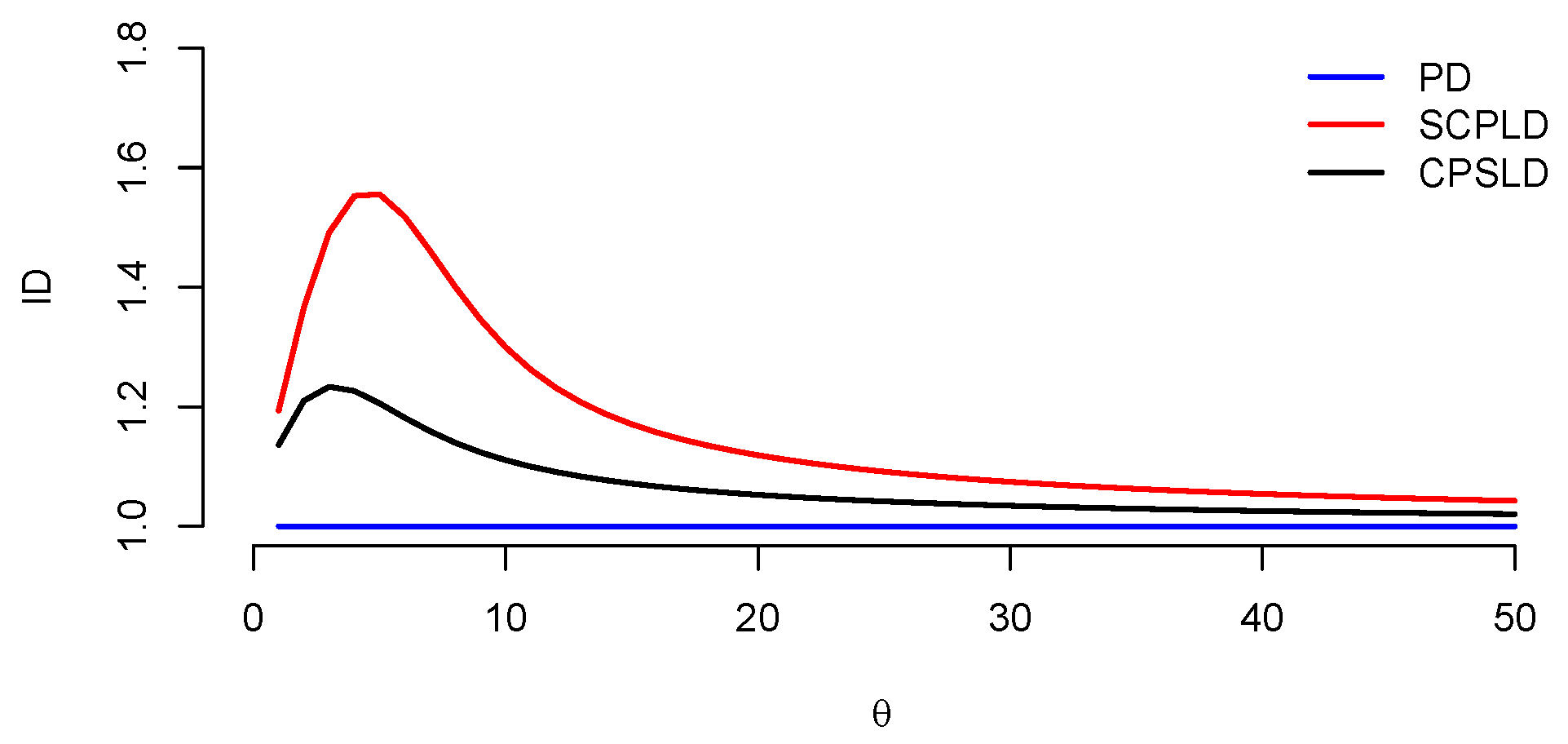
3.2. Index of Dispersion

We calculated the values of the index of dispersion (ID) for PD, SCPLD, and CPSLD for different values of $\theta$. To assess the dispersion of a distribution, the ID is defined as follows:

Definition 4.

The index of dispersion (ID) is defined as

$$\mathit{ID}={\displaystyle \frac{Var\left(X\right)}{E\left(X\right)}}$$

Note: the distribution is overdispersed if $\mathrm{ID}>1$, underdispersed if $\mathrm{ID}<1$, and shows equidispersion if $\mathrm{ID}=1$ (for example, PD). For further details, see [17].

The ID values of the PD, SCPLD, and CPSLD are visualized in Figure 2. One can observe that both SCPLD and CPSLD are overdispersed. Furthermore, the SCPLD is more dispersed than the CPSLD; in fact, ${\mathrm{ID}}_{\mathrm{SCPLTD}}>{\mathrm{ID}}_{\mathrm{CPSLTD}}>{\mathrm{ID}}_{\mathrm{PD}}$. The maximum value of the ID for SCPLD is $1.5554$ at $\theta =4.1$ and the maximum value of the ID for CPSLD is $1.2338$ at $\theta =3.1$.

3.3. Unimodality

We noted in Figure 1 that the pmfs of the CPLD decrease for $\theta \le 4$ and are unimodal with proper mode for $\theta \ge 4$. Thus, in this subsection, the unimodality property of the distributions under study is investigated such that we prove that the CPLD is a unimodal distribution as follows:

Theorem 2.

The CPLD has a unimodal distribution.

Proof. 

Note that the pmf in Equation (2) of the CPLD is unimodal if and only if $f\left(x\right)-f(x+1)$ has at most one sign change, and if such a sign change occurs, it should be a negative value to positive value. Now, we have

$$f\left(x\right)-f(x+1)={\displaystyle \frac{{\theta }^x}{x(x+1)(x+1)!C\left(\theta \right)}}\left[{(x+1)}^2-\theta x\right].$$

Thus, the sign is determined by studying the sign of the quantity $h\left(x\right)={(x+1)}^2-\theta x$. Note that for $\theta \le 4$, ${(x+1)}^2-\theta x\ge {(x+1)}^2-4x={(x-1)}^2\ge 0$ and hence, $h\left(x\right)\ge 0$. This implies that $f\left(x\right)$ is decreasing for $\theta \le 4$ as for $x\ge 1$ then $h\left(x\right)\ge 0$. For the following, we assume that $\theta >4$. Now, for $x\ge (\theta -2)$, $h\left(x\right)\ge {(x+1)}^2-x(x+2)=1>0$. Also, as $x\ge 1$ then for $x\le (\theta -3)$, $h\left(x\right)\le {(x+1)}^2-x(x-3)=1-x\le 0$. Therefore, one has

$$f\left(x\right)\le f(x+1)\mathrm{for}x\le (\theta -3).$$

and

$$f\left(x\right)\ge f(x+1)\mathrm{for}x\ge (\theta -2).$$

Hence, the mode is $(\theta -2)$ when $\theta$ is a positive integer; otherwise, one or both of the two integers lying in the interval $(\theta -3,\theta -1)$ are modes. □

The plots in Figure 3 illustrate the pmfs of the PD, the CPSLD, and the SCPLD at different values of the mean $\mu =3,5,10,15$. For $\mu =3$, the SCPLD shows the highest probability for small values of y, followed by the CPSLD, while the PD gets less probability for small counts. As the mean increases to $\mu =5$, the differences between the distributions start to reduce. For $\mu =10$ and $\mu =15$, the pmfs of the PD, CPSLD, and SCPLD become nearly identical, showing symmetric bell-shaped patterns centered around their means. This suggests that structural differences between the models become not as significant as $\mu$ increases and their behavior converges.

Theorem 3.

The CPLD is strongly unimodal and hence has an increasing failure rate function.

Proof. 

To prove that the CPLD is strongly unimodal and has an increasing failure rate, we need to prove that the CPLD is log-concave. Then, we have

$$\mathrm{\Phi }\left(x\right)={\displaystyle \frac{f(x+1)}{f\left(x\right)}}={\displaystyle \frac{\theta x}{{(x+1)}^2}},x=1,2,...$$

Taking the derivative with respect to y, one gets

$${\displaystyle \frac{\partial \mathrm{\Phi }\left(x\right)}{\partial x}}={\displaystyle \frac{\theta (1-x)}{{(x+1)}^3}},x=1,2,...$$

Since $1-x\le 0$ for all $x=1,2,...$, we get ${\displaystyle \frac{\partial \mathrm{\Phi }\left(x\right)}{\partial x}}\le 0$. Consequently, $\mathrm{\Phi }\left(x\right)$ is decreasing. Therefore, the CPLD is log-concave. Then, the CPLD is strongly unimodal. In addition, the CPLD has an increasing failure rate based on the fact that if pmf is log-concave, then the failure rate function is monotone increasing; see [9,18,19] for more information. □

From Theorem 3, we conclude that the SCPLD also has a log-concave distribution. Consequently, it exhibits strong unimodality and has an increasing failure rate function.

Theorem 4.

The CPSLD is strongly unimodal and has an increasing failure rate.

Proof. 

First, we need to prove that the CPSLD is log-concave. Then, we have

$$\mathrm{\Phi }\left(x\right)={\displaystyle \frac{f(x+1)}{f\left(x\right)}}={\displaystyle \frac{\theta }{x+2}}$$

which clearly is decreasing in x. Therefore, the CPSLD has a log-concave distribution. Then, the CPSLD is strongly unimodal, and it also has an increasing failure rate function. □

Remark 3.

Although the PD and CPLD (SCPLD) share the property of strong unimodality, the PD is ultra log-concave (a property stronger than strong unimodality), but the CPLD (SCPLD) is not.

3.4. Stochastic Ordering

In this subsection, we study the stochastic ordering of the distributions considered. The following is a definition of likelihood ratio stochastic order:

Definition 5.

Let $X_1$ and $X_2$ be two discrete random variables with pmfs $f\left(x\right)$ and $g\left(x\right)$, respectively. We say that $X_1$ is smaller than $X_2$ in the likelihood ratio order (denoted by $X_1{\le }_{lr}{X}_2$) if ${\displaystyle \frac{g\left(x\right)}{f\left(x\right)}}$ increases in x over the union of the supports of $X_1$ and $X_2$.

It is well known that the likelihood ratio order implies hazard and stochastic orders; see [20] for more details.

Theorem 5.

Let $X_1$ and $X_2$ be two random variables following CPLD (SCPLD, CPSLD) with parameters ${\theta }_1$ and ${\theta }_2$, respectively. If ${\theta }_1\le {\theta }_2$, then $X_1{\le }_{lr}{X}_2$.

Proof. 

Let $f_{\theta }\left(x\right)$ be pmf of the CPLD with parameter $\theta$. Then, we have

$${\displaystyle \frac{f_{{\theta }_2}\left(x\right)}{f_{{\theta }_1}\left(x\right)}}=A({\theta }_1,{\theta }_2){({\displaystyle \frac{{\theta }_2}{{\theta }_1}})}^x.$$

where $A({\theta }_1,{\theta }_2)$ is a function of ${\theta }_1$ and ${\theta }_2$ and does not depend on x. Hence, the ratio increases in x if and only if ${\theta }_1\le {\theta }_2$. This implies that $X_1{\le }_{lr}{X}_2$. The proofs for the cases of SCPLD and CPSLD are similar. □

Note that $X_1{\le }_{\mathrm{lr}}{X}_2$ implies that $X_1{\le }_{\mathrm{st}}{X}_2$ when ${\theta }_1\le {\theta }_2$. Then, we conclude that $E\left(X_1\right)\le E\left(X_2\right)$. Hence, we have an alternative proof of Remark 2. In fact, moments of all orders increase in $\theta$.

Theorem 6.

Let $X_1,X_2$, and $X_3$ be three random variables following SCPLD, CPSLD, and PD with the same parameter θ, respectively. Then, $X_1{\le }_{lr}{X}_2{\le }_{lr}{X}_3$.

Proof. 

We have

$${\displaystyle \frac{f_{\mathrm{CPSLD}}\left(x\right)}{f_{\mathrm{SCPLD}}\left(x\right)}}=B\left(\theta \right)(x+1).$$

(3)

where $B\left(\theta \right)$ is a function of $\theta$ and does not depend on x. Hence, the ratio is increasing in x. This implies $X_1{\le }_{lr}{X}_2$.

Similarly,

$${\displaystyle \frac{f_{\mathrm{PD}}\left(x\right)}{f_{\mathrm{CPSLD}}\left(x\right)}}=C\left(\theta \right)(x+1).$$

(4)

where $C\left(\theta \right)$ is a function of $\theta$ and does not depend on x. Hence, the ratio is increasing in x. This implies $X_2{\le }_{lr}{X}_3$. From Equations (3) and (4), we can conclude that $X_1{\le }_{lr}{X}_2{\le }_{lr}{X}_3$.

Hence, the distribution is also ordered with respect to the hazard rate and the usual stochastic orders. □

4. Parametric Estimation and Simulation Study

An estimation of the CPLD and CPSLD parameters using the method of moments (MM) and the maximum likelihood (ML) method is addressed in this section.

4.1. Estimation Study of CPLD

The MM estimate for $\theta$ is obtained as the solution of the following equation:

$$E\left(X\right)=\overline{x},$$

where $\overline{x}$ is the sample mean. Hence, we have the following equation

$${\displaystyle \frac{e^{\widehat{\theta }}-1}{C\left(\widehat{\theta }\right)}}-\overline{x}=0.$$

(5)

Then, the MM estimate can be calculated by solving Equation (5) numerically.

For the ML method, the likelihood function is given by

$$L(\theta ;x_1,x_2,\dots ,x_n)={\displaystyle \frac{{\theta }^{{\sum }_{i=1}^n{x}_i}}{C{\left(\theta \right)}^n}}\prod _{i=1}^n{\displaystyle \frac{1}{x_i{x}_i!}},$$

(6)

Then, the log likelihood function is given from Equation (6) as follows:

$$𝓁\left(\theta \right)=𝓁(\theta ;x_1,x_2,\dots ,x_n)\propto -nlogC\left(\theta \right)+log\theta \sum _{i=1}^n{x}_i,$$

(7)

The ML estimate is obtained as a solution to numerically maximize the score function using a Newten-type algorithm; refer to [21] for additional details regarding the algorithm. This leads to a solution for Equation (5) and, hence, the ML estimator for $\theta$ is identical to that of the MM estimator.

4.2. Simulation Study for CPLD

This simulation study provides a numerical assessment of the estimates of the proposed parameters. A simulation study was conducted to evaluate the efficiency of the ML estimates of the parameter $\theta$. A total of 1000 Monte Carlo replications were conducted, with sample sizes of $n=10,20,50,100$, and 500, along with parameter values $\theta$ = 0.5, 1, and 5. The simulation was executed in the following steps:

• Choose the value $\theta$ and the sample size n.
• Generate n random samples such that $X\sim CPLD$.
• Maximize Equation (6) to find the ML estimate for $\theta$ numerically.
• Repeat steps 2 to 3 for $N=1000$ times to calculate the following:
  • The absolute bias of the simulated estimates is defined as

    $$\left|\mathrm{Bias}\right|(\widehat{\theta })={\displaystyle \frac{1}{N}}\sum _{i=1}^N|\widehat{\theta }-\theta |$$
  • The average of the mean squared error of the simulated estimates is defined as

    $$\mathrm{MSE}(\widehat{\theta })={\displaystyle \frac{1}{N}}\sum _{i=1}^N{(\widehat{\theta }-\theta )}^2$$

The simulation results are shown in

Table 1. The ML outcomes of the CPLD for various $\theta$ values.

n	$\mathit{\theta }$	$\widehat{\mathit{\theta }}$	|Bias|	MSE
10		0.4846	0.0154	0.0394
20		0.4916	0.0083	0.0079
50	0.5	0.4939	0.0061	0.0042
100		0.4966	0.0034	0.00203
500		0.4986	0.0014	0.0016
10		0.9976	0.0024	0.0536
20		0.9998	0.0002	0.0045
50	1	1.0001	0.0001	0.0003
100		0.9998	0.0001	0.0002
500		0.9999	0.00008	0.0001
10		5.0088	0.0088	0.1111
20		4.9997	0.0003	0.0112
50	5	5.0001	0.0001	0.0008
100		4.9999	0.00003	0.0002
500		4.9999	0.00001	0.00001

. The table includes the following values: the true value of $\theta$, the estimate $\widehat{\theta }$, the absolute bias of $\theta$, and the MSE of $\theta$ for different values of n.

From Table 1, one can conclude the following:

• As the sample size n increases, the estimates values ($\widehat{\theta }$) converge to the true value $\theta$.
• The absolute bias decreases with the increase in sample size n, indicating that the estimates tend to be unbiased estimates.
• The MSE significantly decreases with the increase in sample size n that makes the ML estimates more accurate.

Then, it can be concluded that the ML method provides accurate estimates for the parameter $\theta$ of the CPLD.

4.3. Estimation Study of CPSLD

The MM estimate for $\theta$ is obtained as a solution of the following equation:

$${\displaystyle \frac{e^{\widehat{\theta }}(\widehat{\theta }-1)+1}{e^{\widehat{\theta }}-1}}-\overline{x}=0.$$

(8)

By solving Equation (8) numerically, we get the MM estimates.

For the ML method, the likelihood function is

$$L(\theta ;x_1,x_2,\dots ,x_n)=\prod _{i=1}^n{\displaystyle \frac{{\theta }^{x_i+1}}{(e^{\theta }-1)(x_i+1)!}},$$

(9)

The log likelihood function is obtained from Equation (9) as follows:

$$𝓁\left(\theta \right)=𝓁(\theta ;x_1,x_2,\dots ,x_n)=\sum _{i=1}^n\left[(x_i+1)log\theta -log(e^{\theta }-1)-log((x_i+1)!)\right],$$

(10)

The ML estimate is obtained as a solution of the score function numerically, which is the same as (8).

4.4. Simulation Study for CPSLD

In this simulation study, the exact technique and steps for simulation detailed in Section 4.2 are executed except for the following:

• In step 2, n random samples were obtained from the CPSLD.
• In step 3, the score function used is presented in Equation (9).

• The simulation results are shown in

  Table 2. The ML results of the CPSLD for different values of $\theta$.

  n	$\mathit{\theta }$	$\widehat{\mathit{\theta }}$	|Bias|	MSE
  10		0.4805	0.0195	0.0884
  20		0.4873	0.0126	0.0407
  50	0.5	0.5022	0.0022	0.0176
  100		0.4980	0.0019	0.0086
  500		0.4993	0.0007	0.0014
  10		1.0028	0.0028	0.1525
  20		0.9981	0.0019	0.0073
  50	1	0.9985	0.0014	0.0065
  100		1.0011	0.0011	0.0051
  500		0.9996	0.0004	0.0025
  10		4.9892	0.0107	0.1756
  20		4.9911	0.0089	0.0255
  50	5	4.9994	0.0006	0.0177
  100		5.0003	0.0003	0.0005
  500		5.00005	0.00005	0.00008

  below.

From Table 2, one can observe that we reach a similar conclusion as in Section 4.2 in terms of the ML estimates based on the absolute bias and the MSE. For instance, the absolute bias and the MSE decrease as the sample sizes n increase, making ML estimates favorable and consistent.

5. Applications

This section examines the performance of CPLD, SCPLD, and CPSLD by comparing them to other distributions and applying real-life data sets. The ML method was employed to obtain parameter estimates for these distributions. The Akaike information criterion (AIC) and the Bayesian information criterion (BIC) were used as comparison tools. The AIC and BIC formulas can be expressed in practical terms as follows:

$$AIC=-2{𝓁}^{*}+2t$$

and

$$BIC=-2{𝓁}^{*}+tlog\left(n\right)$$

Note that ${𝓁}^{*}$ is the estimation of ℓ and t is the number of parameters. In general, the smaller the values of these statistics, the better the fit to the data. In addition, the chi-squared test is provided with corresponding p-values. Calculations are performed using the R programming language.

5.1. Number of Eggs per Flower Head

In comparison to the zero-truncated Poisson distribution (ZTPD) in [22], the zero-truncated Poisson Lindley distribution (ZTPLiD) exhibits a superior fit for data concerning the number of eggs per flower head. However, ref. [11] showed that the CNBLD demonstrated a better fit to the data in comparison to the ZTPLiD and ZTPD, as proven by their lower AIC and BIC values. The mean, variance, and ID related to this data are calculated as 3.0340, 3.3436, and 1.1020, respectively. These values suggest the existence of overdispersion. We observed that the LD has an impact on the CPLD by progressively increasing the probability of small values of X when comparing the observed frequencies of the ZTPLiD, ZTPD, CNBLD, and CPLD in

Table 3. The number of counts of flower heads as per the number of fly eggs.

X	OF 1	ZTPD	ZTPLiD	CNBLD	CPLD
1	22	15.28	26.78	21.42	19.92
2	18	21.86	19.77	19.79	19.92
3	18	20.84	13.94	16.81	17.71
4	11	14.90	9.53	12.45	13.28
5	9	8.53	6.37	8.12	8.50
6	6	4.06	4.19	4.73	4.72
7	3	1.66	2.72	2.51	2.31
8	0	0.59	1.74	1.22	1.02
9	1	0.19	1.11	0.55	0.40
Total	88
ML		$\widehat{\theta }=2.8604$	$\widehat{\theta }=0.7186$	$\widehat{\theta }=0.1267$	$\widehat{\theta }=4.0004$
				$\widehat{r}=28.1719$
AIC		335.09	336.76	331.93	329.93
BIC		337.57	339.24	336.89	332.41

¹ OF = observed frequency.

. In addition, Table 3 clearly shows that the CPLD provided a better fit to the data with lower AIC and BIC values.

5.2. Number of European Corn Borers

Data from the entomological field involving the number of European corn borers were discussed in several studies. For example, ref. [23] reported the results of fitting NB, Neyman’s type A (NTA), and Poisson binomial (PB) distributions using the chi-squared test for goodness of fit, as shown in

Table 4. Goodness of fit results for NB, NTA, and PB for the number of European corn borers in [23].

X	OF 1	NB	NTA	PB
0	188	185.79	187.99	197.02
1	83	89.28	85.02	84.34
2	36	32.99	34.52	37.45
3	14	10.97	11.65	11.17
4	2	3.45	3.51	3.11
5	1	1.52	1.30	0.91
Total	88
${\chi }^2$		2.36	1.28	1.06
p-value		0.505	0.735	0.785
d.f		3

¹ OF = observed frequency.

. According the results in Table 4, ref. [23] claimed that PB distribution is the best fitting distribution for the data. In addition, ref. [3] considered the PD, PLiD, and PAD for modeling the number of European corn borers. In another study [3], the PLiD fits the data better than the PD and PAD.

Table 5. The number of European corn borers.

X	OF 1	PD	PLiD	PAD	SCPLD	CPSLD
0	188	169.46	194.05	197.53	187.47	177.94
1	83	109.83	79.53	75.72	85.47	97.77
2	36	35.59	31.32	30.23	34.64	35.81
3	14	7.69	11.99	12.26	11.84	9.84
4	2	1.25	4.50	4.97	3.46	2.16
5	1	0.18	2.61	3.29	1.12	0.46
Total	324
ML($\widehat{\theta }$)		0.65	2.04	2.09	1.82	1.10
−2log ℓ		724.49	714.09	716.74	710.54	714.08
AIC		726.49	716.09	718.74	712.54	716.07
BIC		730.27	719.88	722.52	716.32	719.86
${\chi }^2$		15.4056	1.2719	2.8647	0.1472	4.4469
p-value		0.0005	0.5294	0.2387	0.9290	0.1082
d.f		2

¹ OF = observed frequency.

shows the results of fitting the data of the number of European corn borers, including the ML estimates, AICs, BICs, ${\chi }^2$ statistics, and p-values. From Table 4 and Table 5, it is obvious that the SCPLD gives the best fit for the data in terms of the AIC and BIC criteria and the chi-squared test compared to the PD, PLiD, and PAD in [23]. In addition, the SCPLD is better than NB, NTA, and PB distributions in terms of the chi-squared test.

5.3. Number of Micronuclei Counted Using Cytochalasin B Method After 4 Gy Irradiation Exposure

The data set represents the number of micronuclei after exposure at a dose of 4 Gy of $\gamma$ radiation, counted using the cytochalasim B method and available in [24]. It is used to assess the performance of the models under study. The study [24] confirmed that the Poisson area-biased Ailamujia distribution (PABAD) performs better than size-biased Poisson Ailamujia distribution (PSBAD), Poisson Ailamujia distribution (PAiD), PD, PLiD, and Poisson Shanker distribution (PSD). In

Table 6. The number of micronuclei after exposure at a dose of 4 Gy of $\gamma$ radiation.

X	OF 1	PD	PLiD	PAiD	PABAD	PSBAD	PSD	SCPLD	CPSLD
0	1974	1816.01	2396.79	2412.91	2027.28	2089.44	2398.31	2031.23	2010.23
1	1674	1839.97	1300.33	1256.24	1638.94	1582.51	1288.41	1600.37	1619.55
2	869	932.12	668.81	664.62	828.12	799.09	665.14	857.57	869.87
3	342	314.81	332.15	343.20	334.74	336.23	334.03	351.47	350.41
4	102	79.74	160.91	171.34	118.39	127.33	164.38	117.47	112.92
5	26	16.16	76.52	82.79	38.29	45.01	79.65	33.34	30.33
6	13	2.73	35.87	38.88	11.61	15.15	38.12	8.26	6.98
7	2	0.39	30.59	17.81	3.35	4.92	33.93	2.27	1.70
Total	5002
ML($\widehat{\theta }$)		1.01319	1.3873	1.7323	1.9739	1.4804	1.3197	2.5160	1.6113
−2log ℓ		13,535.82	13,836.73	13,895.01	6740.37	6752.8	6931.20	13,478.64	13,475.52
AIC		13,537.82	13,838.73	13,897.01	13,482.3	13,507.2	13,862.41	13,480.64	13,477.52
BIC		13,544.34	13,845.25	13,903.53	13,489.5	13,514.3	13,864.41	13,487.15	13,484.04
${\chi }^2$		92.7039	336.95	379.28	11.25	32.98	358.14	10.9582	8.9499
p-value		≈0	≈0	≈0	0.128	≈0	≈0	0.0522	0.1111
d.f		5

¹ OF = observed frequency.

, the results show that both the AIC and BIC values for SCPLD and CPSLD are smaller than the AIC and BIC values for PABAD. In addition, the $p$-values of the chi-square test for SCPLD and CPSLD are significant. As a result, the SCPLD and CPSLD are convenient models to fit this data.

6. Conclusions

In conclusion, this paper introduces a new distribution for count data using the concept of conflating probability distributions. The proposed distribution is termed the conflation of PD and LD (CPLD). The CPLD, characterized by a single parameter and derived from a logarithmic probability mass function as a weighting function and a PD as a parent distribution, inherits properties from both distributions.

Two modifications of the CPLD were investigated, namely the SCPLD and CPSLD that offer enhanced flexibility and the ability to model a broader range of data compared to the CPLD due to the inclusion of zero counts. In order to explore the statistical characteristics for CPLD, SCPLD, and CPSLD, an investigation was conducted.

Furthermore, we examined the estimation of the CPLD and CPSLD parameters using the MM and ML algorithms. The simulation studies were employed to evaluate the efficacy of the estimations provided by the ML method. The ML estimates were consistent, as evidenced by the simulation results. The paper demonstrates that these new distributions are more effective at modeling real count data compared to traditional count distributions such as PD and NBD, as well as other discrete distributions. It highlights their wide applicability across diverse fields. Developing new conflated distributions from other discrete distributions and testing their validity with real-world data is the next challenge in this field of research.

References

1. Greenwood, M.; Yule, G.U. An inquiry into the nature of frequency distributions representative of multiple happenings with particular reference to the occurrence of multiple attacks of disease or of repeated accidents. J. R. Stat. Soc. 1920, 83, 255–279. [Google Scholar] [CrossRef]
2. Sankaran, M. The Discrete Poisson-Lindley Distribution. Biometrics 1970, 26, 145–149. [Google Scholar] [CrossRef]
3. Shanker, R.; Fesshaye, H.; Tesfazghi, T. On Poisson-Akash distribution and its applications. Biom. Biostat. Int. J. 2016, 3, 146–153. [Google Scholar] [CrossRef]
4. Shanker, R.; Fesshaye, H.; Shanker, R.; Leonida, T.A.; Sium, S. On discrete Poisson-Shanker distribution and its applications. Biom. Biostat. Int. J. 2017, 5, 00121. [Google Scholar] [CrossRef]
5. Conway, R.W.; Maxwell, W.L. Network dispatching by the shortest-operation discipline. Oper. Res. 1962, 10, 51–73. [Google Scholar] [CrossRef]
6. Shmueli, G.; Minka, T.P.; Kadane, J.B.; Borle, S.; Boatwright, P. A useful distribution for fitting discrete data: Revival of the Conway–Maxwell–Poisson distribution. J. R. Stat. Soc. Ser. C Appl. Stat. 2005, 54, 127–142. [Google Scholar] [CrossRef]
7. Fisher, R.A. The effect of methods of ascertainment upon the estimation of frequencies. Ann. Eugen. 1934, 6, 13–25. [Google Scholar] [CrossRef]
8. Rao, C.R. On discrete distributions arising out of methods of ascertainment. Sankhyā Indian J. Stat. Ser. A 1965, 27, 311–324. [Google Scholar]
9. Johnson, N.L.; Kemp, A.W.; Kotz, S. Univariate Discrete Distributions, 3rd ed.; John Wiley & Sons: Hoboken, NJ, USA, 2005. [Google Scholar] [CrossRef]
10. Hill, T. Conflations of probability distributions. Trans. Am. Math. Soc. 2011, 363, 3351–3372. [Google Scholar] [CrossRef]
11. Alqefari, A.A.; Alzaid, A.A.; Qarmalah, N. On the Conflation of Negative Binomial and Logarithmic Distributions. Axioms 2024, 13, 707. [Google Scholar] [CrossRef]
12. Abramowitz, M.; Stegun, I.A. Handbook of Mathematical Functions with Formulas, Graphs, and Mathematical Tables, 10th ed.; US Government Printing Office: Washington, DC, USA, 1968. [Google Scholar]
13. Butler, R.J.; McDonald, J.B. Using incomplete moments to measure inequality. J. Econom. 1989, 42, 109–119. [Google Scholar] [CrossRef]
14. Winkler, R.L.; Roodman, G.M.; Britney, R.R. The determination of partial moments. Manag. Sci. 1972, 19, 290–296. [Google Scholar] [CrossRef]
15. Karlin, S. Total Positivity; Stanford University Press: Redwood City, CA, USA, 1968. [Google Scholar]
16. Barlow, R.E.; Proschan, F. Statistical Theory of Reliability and Life Testing: Probability Models; Holt, Rinehart and Winston: New York, NY, USA, 1975. [Google Scholar]
17. Sellers, K.F. The Conway-Maxwell-Poisson Distribution, 1st ed.; Cambridge University Press: Shaftesbury Road, UK, 2023. [Google Scholar] [CrossRef]
18. Bagnoli, M.; Bergstrom, T.C. Log-concave probability and its applications. Econ. Theory 2005, 26, 445–469. [Google Scholar] [CrossRef]
19. Bertin, E.M.; Cuculescu, I.; Theodorescu, R. Unimodality of Probability Measures, 1st ed.; Springer: Dordrecht, The Netherlands, 2013. [Google Scholar] [CrossRef]
20. Shaked, M.; Shanthikumar, J.G. Stochastic Orders, 1st ed.; Springer: New York, NY, USA, 2007. [Google Scholar] [CrossRef]
21. Dennis, J.E., Jr.; Schnabel, R.B. Numerical Methods for Unconstrained Optimization and Nonlinear Equations; SIAM: Philadelphia, PA, USA, 1996. [Google Scholar]
22. Shanker, R.; Hagos, F.; Sujatha, S.; Abrehe, Y. On zero-truncation of Poisson and Poisson-Lindley distributions and their applications. Biom. Biostat. Int. J. 2015, 2, 1–14. [Google Scholar] [CrossRef]
23. McGuire, J.U.; Brindley, T.A.; Bancroft, T.A. The distribution of European corn borer larvae Pyrausta nubilalis (Hbn.), in field corn. Biometrics 1957, 13, 65–78. [Google Scholar] [CrossRef]
24. Aijaz, A.; Qurat ul Ain, S.; Afaq, A.; Tripathi, R. Poisson area-biased Ailamujia Distribution and its applications in environmental and medical sciences. Stat. Transit. New Ser. 2022, 23, 167–184. [Google Scholar] [CrossRef]
Figure 1. The p m f s of the CPLD for different values of θ .
Axioms 14 00518 g001
Figure 2. The ID for PD, SCPLD, and CPSLD for different values of θ .
Axioms 14 00518 g002
Figure 3. Comparison of the p m f s of the PD, SCPLD, and CPSLD for different values of μ .
Axioms 14 00518 g003