


Influence Analysis in the Lognormal Regression Model with Fitted and Quantile Residuals


Abstract
1. Introduction
2. Materials and Methods
2.1. The Log-Normal Regression Model
2.2. Log-Normal Regression Residuals
2.2.1. Fitted Residual
2.2.2. Quantile Residual
2.3. Influential Observation Detection Methods
2.3.1. Cook’s Distance (D)
2.3.2. Modified Cook’s Distance (MCD)
2.3.3. Covariance Ratio
2.3.4. Hadi Method
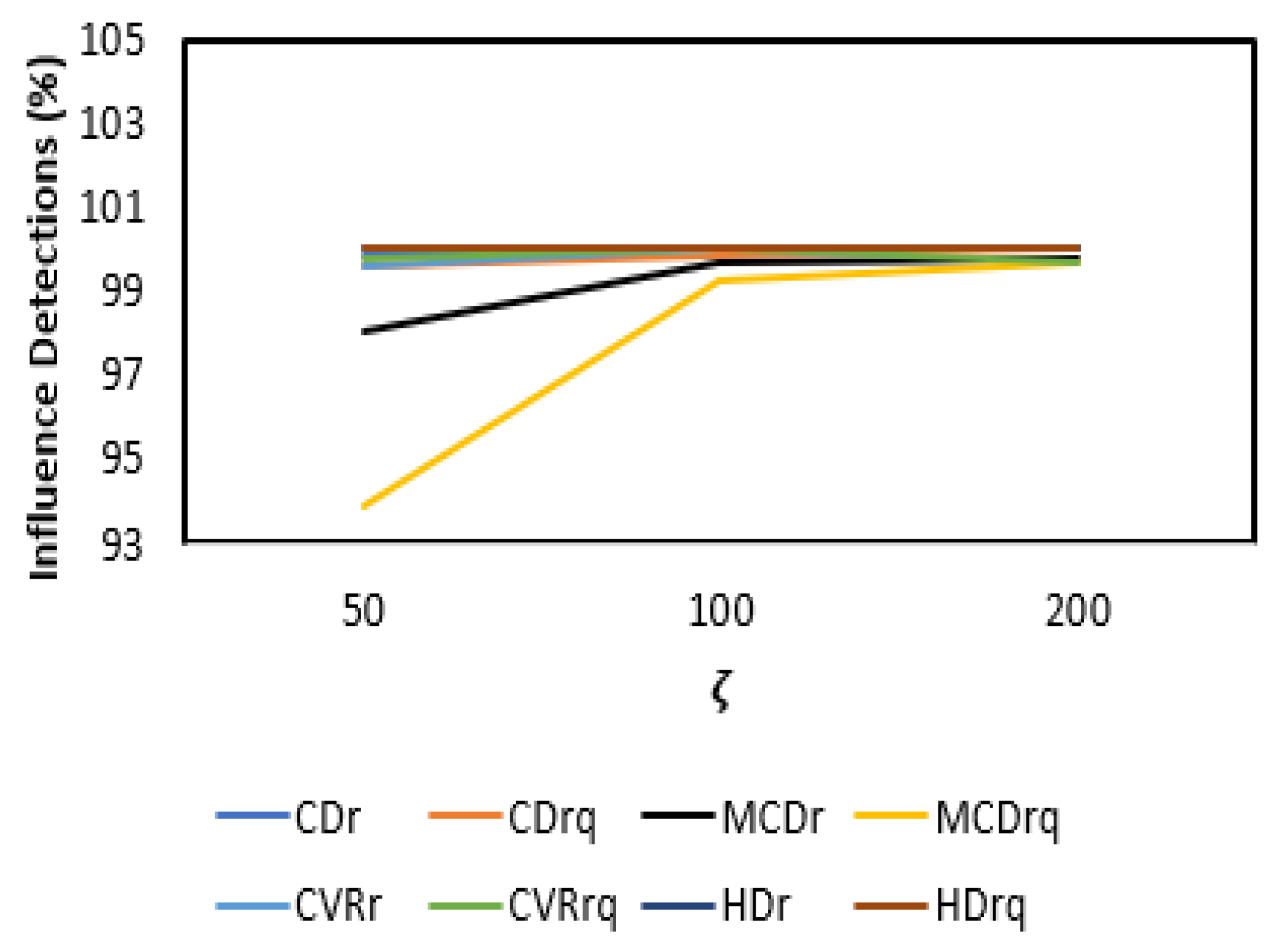
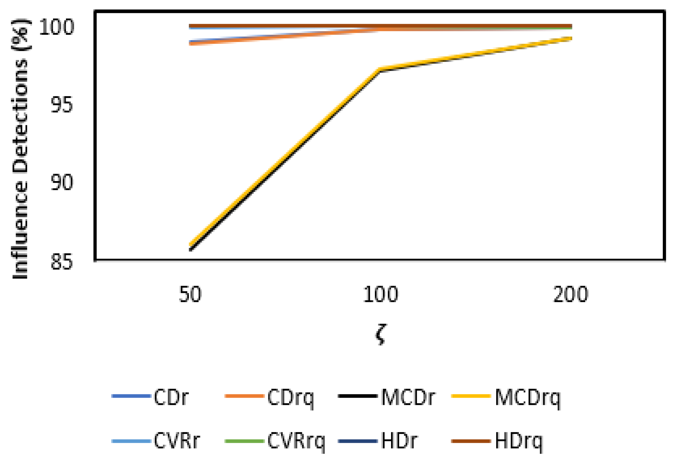
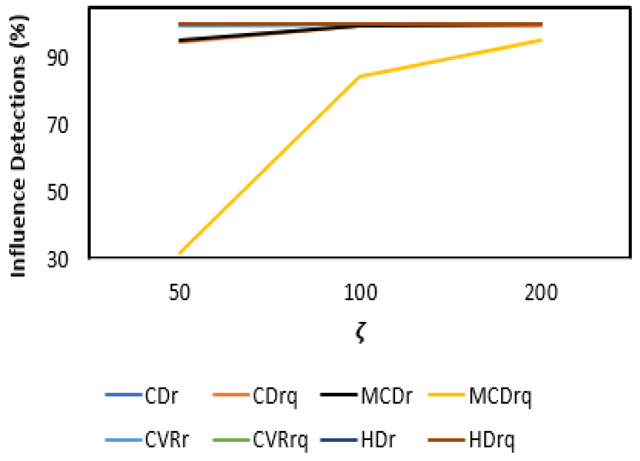
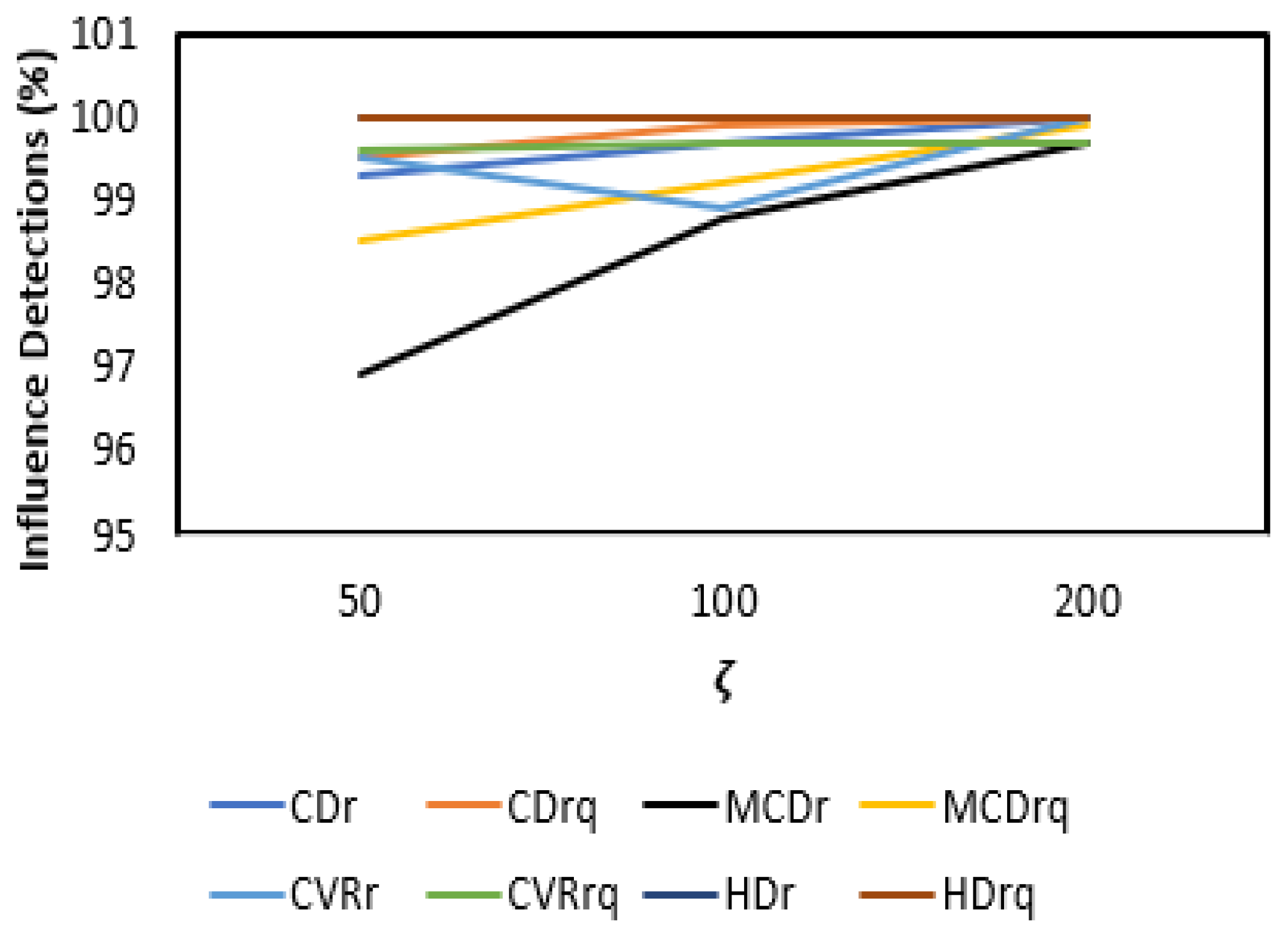
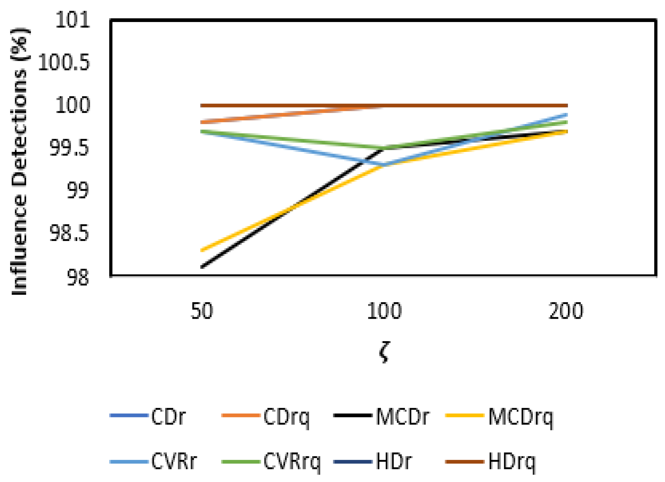
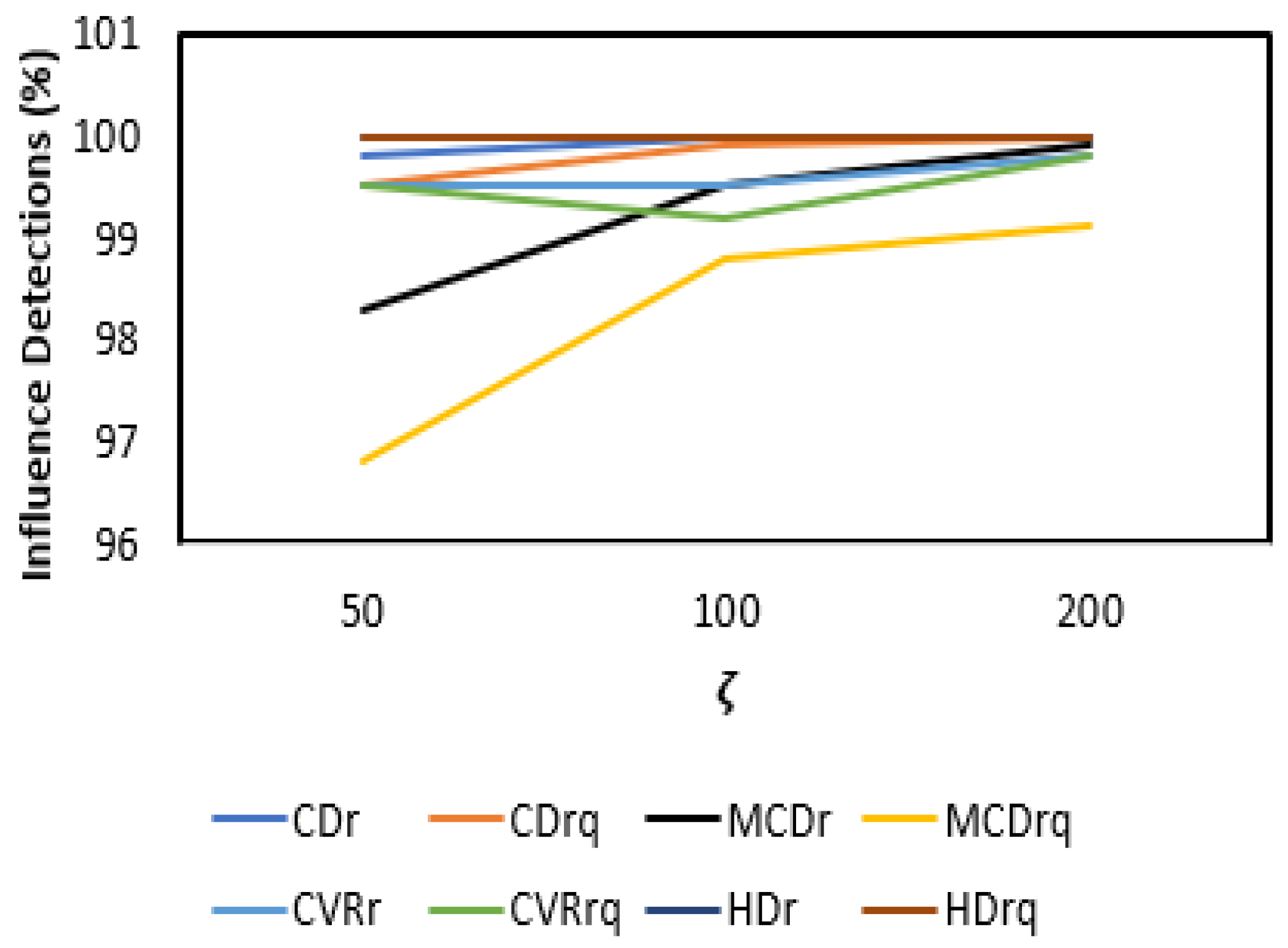
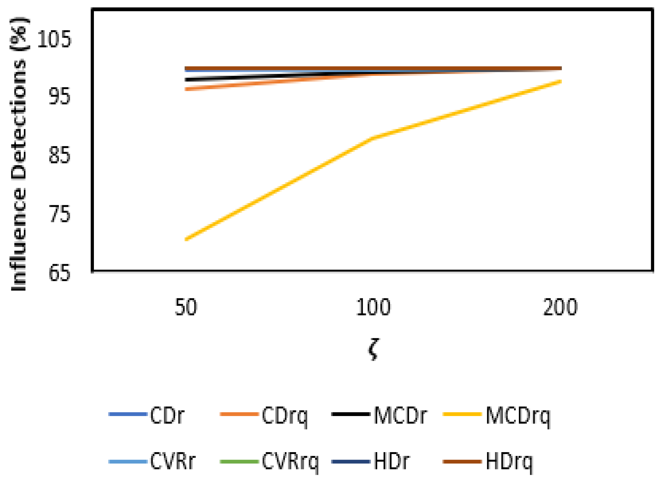
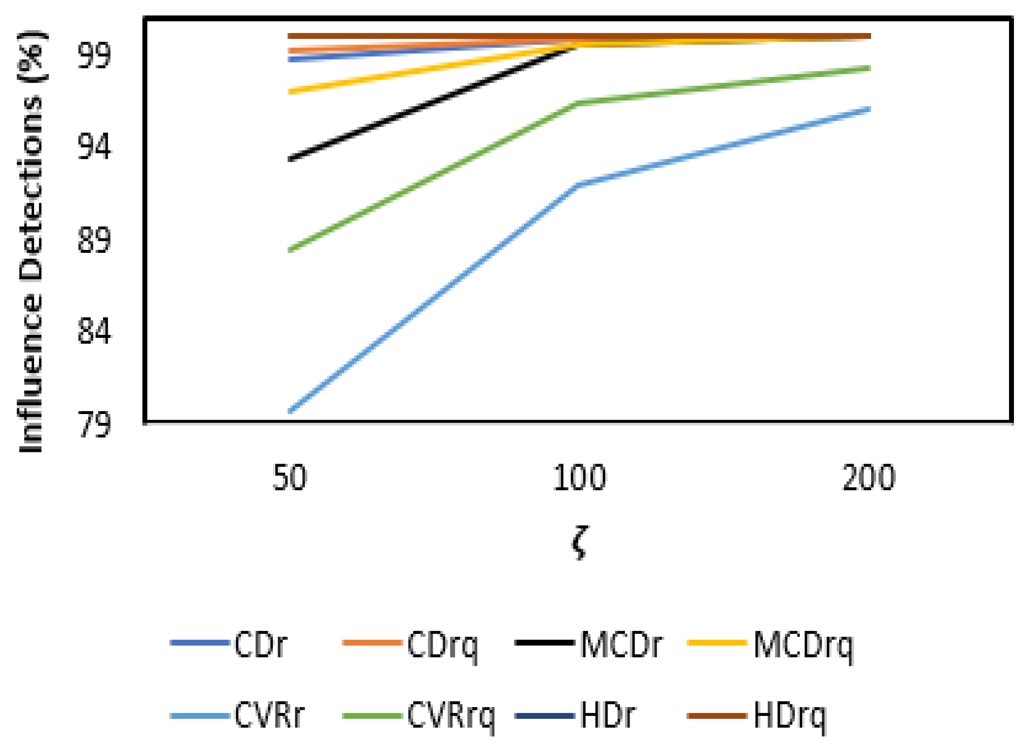
3. Results
3.1. Simulation Layout
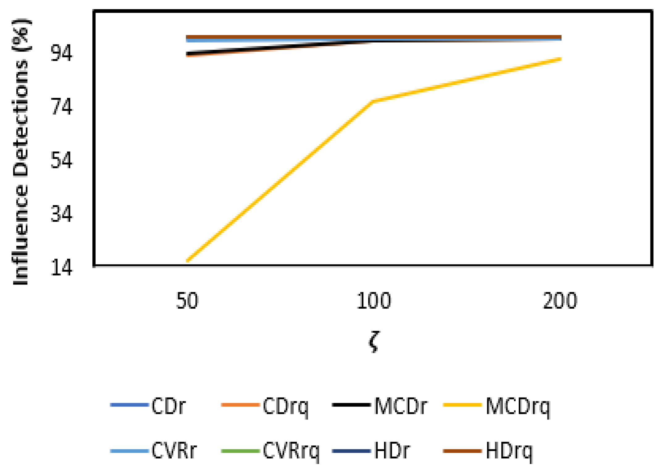
3.2. Results and Discussion
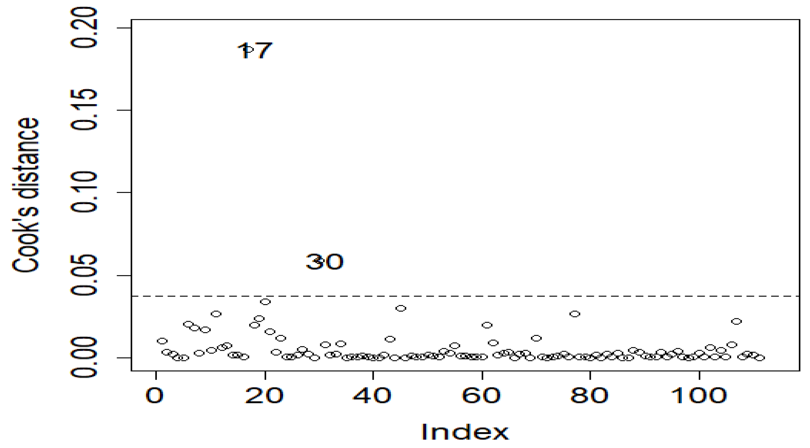
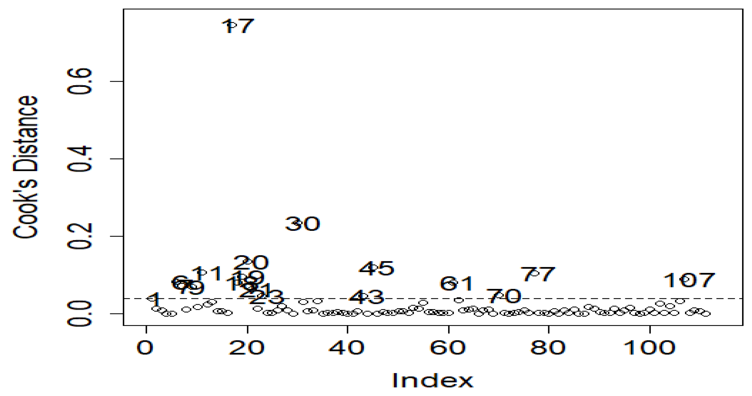
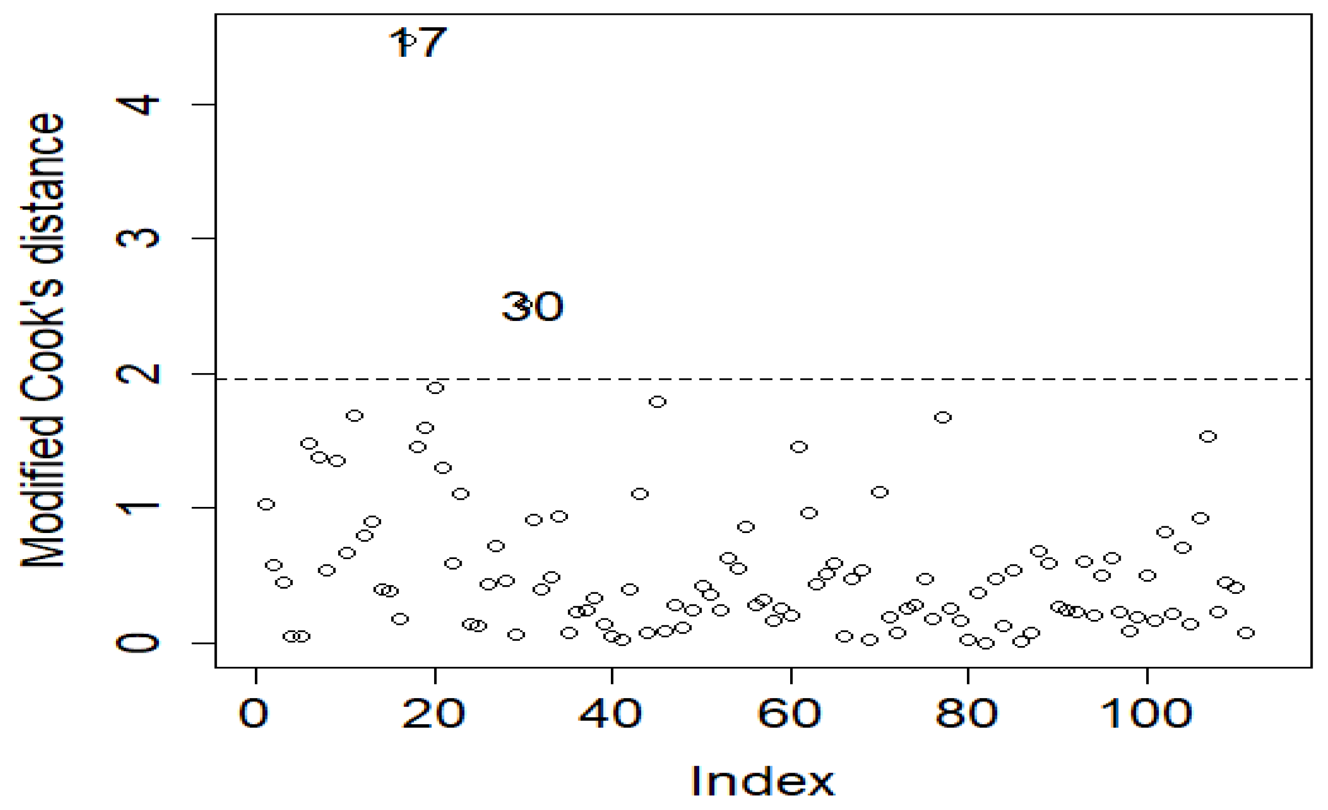
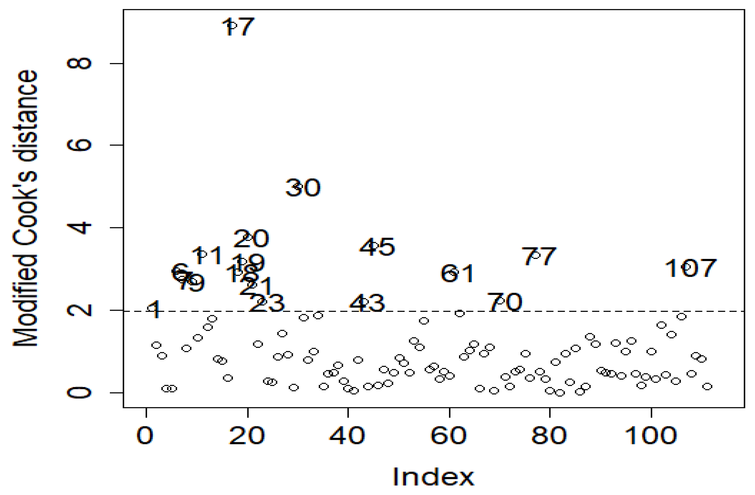
4. Application: Atmospheric Environmental Dataset
5. Conclusions
Author Contributions
Funding
Data Availability Statement
Acknowledgments
Conflicts of Interest
References
- Montgomery, D.C.; Peck, E.A.; Vining, G.G. Introduction to Linear Regression Analysis, 5th ed.; Wiley: Hoboken, NJ, USA, 2012. [Google Scholar]
- Limpert, E.; Stahel, W.A.; Abbt, M. Lognormal distributions across the sciences: Keys and clues. BioScience 2001, 51, 341–352. [Google Scholar] [CrossRef]
- Kleiber, C.; Zeileis, A. Applied Econometrics with R; Springer: New York, NY, USA, 2008. [Google Scholar]
- Cook, R.D. Assessment of local influence. J. R. Stat. Soc. Ser. B 1986, 48, 133–155. [Google Scholar] [CrossRef]
- Xiang, L.; Tse, S.K.; Lee, A.H. Influence diagnostics for generalized linear mixed models: Applications to clustered data. Comput. Stat. Data Anal. 2002, 40, 759–774. [Google Scholar] [CrossRef]
- Hoque, Z.; Khan, S.; Wesolowski, J. Performance of preliminary test estimator under Linex loss function. Commun. Stat. Theory Methods 2009, 38, 252–261. [Google Scholar] [CrossRef]
- Cook, R.D. Detection of influential observation in linear regression. Technometrics 1977, 19, 15–18. [Google Scholar] [CrossRef]
- Chatterjee, S.; Hadi, A.S. Influential observations, high leverage points, and outliers in linear regression. Stat. Sci. 1986, 1, 379–393. [Google Scholar]
- Balasooriya, U.; Daniel, L.; Rao, P.S. Identification of outliers and influential observations in linear regression: A robust approach. Commun. Stat. Simul. Comput. 1987, 16, 647–670. [Google Scholar]
- Brown, G.C.; Lawrence, A.J. Regression diagnostics for the identification of influential observations in linear models. Aust. N. Z. J. Stat. 2000, 42, 451–466. [Google Scholar]
- Meloun, M.; Militký, J. Detection of single influential points in OLS regression model building. Anal. Chim. Acta 2001, 439, 169–191. [Google Scholar] [CrossRef]
- Nurunnabi, A.A.M.; Rahmatullah Imon, A.H.M.; Nasser, M. Identification of multiple influential observations in logistic regression. J. Appl. Stat. 2010, 37, 1605–1624. [Google Scholar] [CrossRef]
- Vanegas, L.H.; Rondón, L.M.; Cordeiro, G.M. Diagnostic tools in generalized Weibull linear regression models. J. Stat. Comput. Simul. 2013, 83, 2315–2338. [Google Scholar] [CrossRef]
- Jang, D.H.; Anderson-Cook, C.M. Firework plots for evaluating the impact of outliers and influential observations in generalized linear models. Qual. Technol. Quant. Manag. 2015, 12, 423–436. [Google Scholar] [CrossRef]
- Zhang, Z. Residuals and regression diagnostics: Focusing on logistic regression. Ann. Transl. Med. 2016, 4, 195. [Google Scholar] [CrossRef]
- Amin, M.; Amanullah, M.; Aslam, M. Empirical evaluation of the inverse Gaussian regression residuals for the assessment of influential points. J. Chemom. 2016, 30, 394–404. [Google Scholar] [CrossRef]
- Bae, W.; Noh, S.; Kim, C. Case influence diagnostics for the significance of the linear regression model. Commun. Stat. Appl. Methods 2017, 24, 155–162. [Google Scholar] [CrossRef]
- Amin, M.; Amanullah, M.; Cordeiro, G.M. Influence diagnostics in the gamma regression model with adjusted deviance residuals. Commun. Stat.-Simul. Comput. 2017, 46, 6959–6973. [Google Scholar] [CrossRef]
- Imran, M.; Akbar, A. Diagnostics via partial residual plots in inverse Gaussian regression. J. Chemom. 2020, 34, e3203. [Google Scholar]
- Khaleeq, J.; Amanullah, M.; Almaspoor, Z. Influence diagnostics in log-normal regression model with censored data. Math. Probl. Eng. 2021, 2021, 1–15. [Google Scholar] [CrossRef]
- Khan, A.; Ullah, M.A.; Amin, M.; Muse, A.H.; Aldallal, R.; Mohamed, M.S. Empirical examination of the Poisson regression residuals for the evaluation of influential points. Math. Probl. Eng. 2022, 2022, 4681597. [Google Scholar] [CrossRef]
- Amin, M.; Fatima, A.; Akram, M.N.; Kamal, M. Influential observation detection in the logistic regression under different link functions: An application to urine calcium oxalate crystals data. J. Stat. Comput. Simul. 2024, 94, 346–359. [Google Scholar] [CrossRef]
- Camilleri, C.; Alter, U.; Cribbie, R.A. Identifying influential observations in multiple regression. Quant. Methods Psychol. 2024, 20, 96–105. [Google Scholar] [CrossRef]
- Soale, A.N. Detecting influential observations in single-index Fréchet regression. Technometrics 2025, 67, 311–322. [Google Scholar] [CrossRef]
- Khan, A.J.; Akbar, A.; Kibria, B.M.G. Influence of residuals on Cook’s distance for Beta regression model: Simulation and application. Hacet. J. Math. Stat. 2025, 54, 618–632. [Google Scholar] [CrossRef]
- Atkinson, A.C. Two graphical displays for outlying and influential observations in regression. Biometrika 1981, 68, 13–20. [Google Scholar] [CrossRef]
- Ajiferuke, I.; Famoye, F. Modelling count response variables in informetric studies: Comparison among count, linear, and lognormal regression models. J. Informetr. 2015, 9, 499–513. [Google Scholar] [CrossRef]
- Paula, G.A. On diagnostics in double generalized linear models. Comput. Stat. Data Anal. 2013, 68, 44–51. [Google Scholar] [CrossRef]
- Dunn, P.K.; Smyth, G.K. Randomized quantile residuals. J. Comput. Graph. Stat. 1996, 5, 236–244. [Google Scholar] [CrossRef]
- Rigby, R.A.; Stasinopoulos, M.D.; Heller, G.Z.; Bastiani, F.D. Distributions for Modeling Location, Scale, and Shape Using GAMLSS in R; CRC Press: New York, NY, USA, 2020. [Google Scholar]
- Pregibon, D. Logistic regression diagnostics. Ann. Stat. 1981, 9, 705–724. [Google Scholar] [CrossRef]
- Ullah, M.A.; Pasha, G.R. The origin and developments of influence measures in regression. Pak. J. Stat. 2009, 25, 295–309. [Google Scholar]
- Hardin, J.W.; Hilbe, J.M. Generalized Linear Models and Extensions, 3rd ed.; Stata Press: College Station, TX, USA, 2012. [Google Scholar]
- Fox, J. An R and S-Plus Companion to Applied Regression; Sage Publications: Thousand Oaks, CA, USA, 2002. [Google Scholar]
- Belsley, D.A.; Kuh, E.; Welsch, R. Regression Diagnostics Identifying Influential Data and Sources of Collinearity; Wiley: New York, NY, USA, 1980. [Google Scholar]
- Hadi, A.S. A New Measure of Overall Potential Influence in Linear Regression. Comput. Stat. Data Anal. 1992, 14, 1–27. [Google Scholar] [CrossRef]
- Kibria, B.M.G.; Månsson, K.; Shukur, G. Performance of Some Logistic Ridge Regression Estimators. Comput. Econ. 2012, 40, 401–414. [Google Scholar] [CrossRef]
- Bruntz, S.M.; Cleveland, W.S.; Graedel, T.E.; Kleiner, B.; Warner, J.L. Ozone concentrations in New Jersey and New York: Statistical association with related variables. Science 1974, 186, 257–259. [Google Scholar] [CrossRef] [PubMed]


| 25 | 0.5 | 99.9 | 99.9 | 99.5 | 99.8 | 99.7 | 99.9 | 100 | 100 |
| 1 | 99.9 | 99.9 | 99.9 | 99.9 | 99.7 | 100 | 100 | 100 | |
| 3 | 100 | 100 | 99.9 | 99.5 | 100 | 100 | 100 | 100 | |
| 9 | 99.9 | 99.6 | 99.7 | 98.5 | 100 | 99.8 | 100 | 100 | |
| 50 | 0.5 | 99.8 | 99.9 | 99.1 | 99.5 | 99.9 | 99.9 | 100 | 100 |
| 1 | 99.9 | 99.9 | 99.4 | 99.3 | 99.7 | 100 | 100 | 100 | |
| 3 | 100 | 99.9 | 99.7 | 99.3 | 100 | 100 | 100 | 100 | |
| 9 | 100 | 99.6 | 99.9 | 97.4 | 100 | 100 | 100 | 100 | |
| 100 | 0.5 | 99.9 | 99.9 | 98.2 | 99 | 99.9 | 99.8 | 100 | 100 |
| 1 | 99.9 | 99.9 | 98.3 | 98.3 | 100 | 99.8 | 100 | 100 | |
| 3 | 100 | 100 | 99.7 | 98.6 | 100 | 99.7 | 100 | 100 | |
| 9 | 100 | 99.6 | 99.7 | 92.6 | 100 | 100 | 100 | 100 | |
| 200 | 0.5 | 100 | 100 | 96.5 | 98.6 | 100 | 99.9 | 100 | 100 |
| 1 | 99.8 | 99.8 | 96.5 | 96.6 | 99.9 | 100 | 100 | 100 | |
| 3 | 100 | 99.9 | 98.4 | 94.4 | 100 | 100 | 100 | 100 | |
| 9 | 100 | 99.4 | 99.4 | 88.3 | 99.8 | 100 | 100 | 100 |
| 25 | 0.5 | 100 | 100 | 99.8 | 99.8 | 99.8 | 99.9 | 100 | 100 |
| 1 | 100 | 100 | 100 | 100 | 100 | 99.7 | 100 | 100 | |
| 3 | 100 | 99.9 | 99.8 | 99.7 | 99.8 | 99.8 | 100 | 100 | |
| 9 | 100 | 99.6 | 99.9 | 98.7 | 99.9 | 99.9 | 100 | 100 | |
| 50 | 0.5 | 99.9 | 99.9 | 99.3 | 99.8 | 99.8 | 100 | 100 | 100 |
| 1 | 100 | 100 | 99.7 | 99.8 | 99.8 | 99.9 | 100 | 100 | |
| 3 | 100 | 100 | 99.7 | 99.2 | 99.8 | 99.6 | 100 | 100 | |
| 9 | 100 | 99.6 | 99.9 | 97.7 | 100 | 99.9 | 100 | 100 | |
| 100 | 0.5 | 99.7 | 99.9 | 98 | 98.7 | 99.9 | 99.9 | 100 | 100 |
| 1 | 100 | 100 | 98.8 | 98.8 | 99.7 | 99.9 | 100 | 100 | |
| 3 | 100 | 99.8 | 99.5 | 98.4 | 99.6 | 99.8 | 100 | 100 | |
| 9 | 100 | 99.5 | 99.7 | 93.4 | 100 | 100 | 100 | 100 | |
| 200 | 0.5 | 99.9 | 99.9 | 96.4 | 98 | 100 | 99.8 | 100 | 100 |
| 1 | 99.8 | 99.8 | 97.2 | 97.3 | 100 | 100 | 100 | 100 | |
| 3 | 100 | 99.9 | 97.9 | 94 | 99.7 | 100 | 100 | 100 | |
| 9 | 100 | 99.5 | 99.6 | 84.1 | 100 | 100 | 100 | 100 |
| 25 | 0.5 | 100 | 100 | 100 | 100 | 99.2 | 99.5 | 100 | 100 |
| 1 | 99.9 | 99.9 | 99.6 | 99.6 | 99.5 | 99.7 | 100 | 100 | |
| 3 | 100 | 99.9 | 99.8 | 99.2 | 99.6 | 99.5 | 100 | 100 | |
| 9 | 100 | 99.7 | 99.9 | 99.1 | 100 | 98.2 | 100 | 100 | |
| 50 | 0.5 | 99.7 | 99.9 | 98.8 | 99.2 | 98.9 | 99.7 | 100 | 100 |
| 1 | 100 | 100 | 99.5 | 99.3 | 99.3 | 99.5 | 100 | 100 | |
| 3 | 100 | 99.9 | 99.5 | 98.8 | 99.5 | 99.2 | 100 | 100 | |
| 9 | 100 | 99.8 | 99.9 | 96.3 | 99.7 | 99.8 | 100 | 100 | |
| 100 | 0.5 | 99.7 | 99.7 | 97 | 99 | 99.2 | 99.7 | 100 | 100 |
| 1 | 99.8 | 99.8 | 98.6 | 98.6 | 99.3 | 100 | 100 | 100 | |
| 3 | 99.8 | 99.6 | 98.7 | 96.3 | 99 | 99.6 | 100 | 100 | |
| 9 | 100 | 98.8 | 99.2 | 87.9 | 99.6 | 100 | 100 | 100 | |
| 200 | 0.5 | 99.7 | 99.9 | 94.5 | 97.8 | 100 | 99.8 | 100 | 100 |
| 1 | 99.7 | 99.7 | 95.9 | 95.9 | 99.8 | 99.4 | 100 | 100 | |
| 3 | 99.8 | 99.4 | 97.5 | 92.5 | 99.8 | 100 | 100 | 100 | |
| 9 | 99.9 | 99 | 99 | 77.2 | 99.4 | 100 | 100 | 100 |
| 25 | 0.5 | 99.8 | 99.9 | 99.5 | 99.6 | 91.9 | 96.3 | 100 | 100 |
| 1 | 99.9 | 99.9 | 99.5 | 99.5 | 94.5 | 94.4 | 100 | 100 | |
| 3 | 99.9 | 99.7 | 99.6 | 98.9 | 97.1 | 90.2 | 100 | 100 | |
| 9 | 100 | 99.1 | 99.8 | 96.7 | 98.5 | 79.9 | 100 | 100 | |
| 50 | 0.5 | 100 | 100 | 99.1 | 99.5 | 98.3 | 99.1 | 100 | 100 |
| 1 | 100 | 100 | 98.6 | 98.6 | 98 | 97.3 | 100 | 100 | |
| 3 | 100 | 99.9 | 99.5 | 98.3 | 99 | 97.1 | 100 | 100 | |
| 9 | 100 | 98.6 | 99.7 | 92.5 | 99.1 | 98.8 | 100 | 100 | |
| 100 | 0.5 | 99.7 | 99.8 | 97.2 | 98.5 | 98.4 | 99.3 | 100 | 100 |
| 1 | 99.9 | 99.9 | 97.4 | 97.5 | 98.9 | 99 | 100 | 100 | |
| 3 | 99.9 | 99.8 | 98.5 | 96.2 | 99 | 98.7 | 100 | 100 | |
| 9 | 100 | 99.3 | 99.5 | 88.7 | 99.7 | 100 | 100 | 100 | |
| 200 | 0.5 | 99.3 | 99.7 | 91.3 | 95 | 99.4 | 99.3 | 100 | 100 |
| 1 | 99.9 | 99.9 | 95.4 | 95.5 | 98.6 | 98.9 | 100 | 100 | |
| 3 | 99.8 | 99.8 | 98.2 | 90.4 | 99.4 | 99.9 | 100 | 100 | |
| 9 | 100 | 99 | 99.1 | 75.9 | 99.2 | 100 | 100 | 100 |
| Probability Distributions | ||||
|---|---|---|---|---|
| Goodness of Fit Tests | Normal | Lognormal | ||
| Statistics | p-value | Statistics | p-value | |
| Anderson-darling | 4.5943 | 0.004511 | 0.44688 | 0.801 |
| Kolmogorov-Smirnov | 0.1513 | 0.01242 | 0.057907 | 0.8507 |
| Cramer-Von Mises | 0.32593 | 0.7337 | 0.13688 | 0.9982 |
| Inf. Obs. | Lognormal Regression Estimates | |||
|---|---|---|---|---|
| 1 | 152.988 | 97.7375 | 101.825 | 94.1318 |
| 4 | 100.804 | 98.781 | 99.1259 | 98.9379 |
| 5 | 97.1943 | 99.1633 | 98.8861 | 99.1343 |
| 6 | 152.684 | 100.517 | 102.281 | 99.5857 |
| 7 | 91.7559 | 102.477 | 99.0024 | 105.552 |
| 9 | 44.1822 | 104.301 | 95.4712 | 102.726 |
| 11 | 165.435 | 102.067 | 102.75 | 98.4527 |
| 17 | 105.55 | 86.0803 | 89.4113 | 111.529 |
| 18 | 122.637 | 104.281 | 99.0503 | 92.3117 |
| 19 | 27.0797 | 94.416 | 95.6552 | 103.407 |
| 20 | 180.588 | 101.772 | 103.497 | 96.9804 |
| 21 | 126.563 | 104.711 | 99.9874 | 99.2246 |
| 23 | 133.837 | 97.3313 | 100.374 | 93.1342 |
| 30 | 34.2729 | 93.7509 | 97.4727 | 114.026 |
| 43 | 108.45 | 102.6 | 98.6887 | 94.6056 |
| 45 | 150.102 | 91.8711 | 102.288 | 91.2524 |
| 61 | 138.806 | 92.5402 | 101.741 | 93.4166 |
| 70 | 119.679 | 103.799 | 99.0141 | 960.832 |
| 77 | 150.942 | 96.5666 | 100.945 | 89.1567 |
| 88 | 71.7297 | 100.884 | 97.4467 | 102.636 |
| 102 | 97.8347 | 99.2629 | 99.428 | 100.854 |
| 107 | 107.326 | 103.962 | 99.5836 | 104.149 |
Disclaimer/Publisher’s Note: The statements, opinions and data contained in all publications are solely those of the individual author(s) and contributor(s) and not of MDPI and/or the editor(s). MDPI and/or the editor(s) disclaim responsibility for any injury to people or property resulting from any ideas, methods, instructions or products referred to in the content. |
© 2025 by the authors. Licensee MDPI, Basel, Switzerland. This article is an open access article distributed under the terms and conditions of the Creative Commons Attribution (CC BY) license (https://creativecommons.org/licenses/by/4.0/).
Share and Cite
Habib, M.; Amin, M.; Aljeddani, S.M.A. Influence Analysis in the Lognormal Regression Model with Fitted and Quantile Residuals. Axioms 2025, 14, 464. https://doi.org/10.3390/axioms14060464
Habib M, Amin M, Aljeddani SMA. Influence Analysis in the Lognormal Regression Model with Fitted and Quantile Residuals. Axioms. 2025; 14(6):464. https://doi.org/10.3390/axioms14060464
Chicago/Turabian StyleHabib, Muhammad, Muhammad Amin, and Sadiah M. A. Aljeddani. 2025. "Influence Analysis in the Lognormal Regression Model with Fitted and Quantile Residuals" Axioms 14, no. 6: 464. https://doi.org/10.3390/axioms14060464
APA StyleHabib, M., Amin, M., & Aljeddani, S. M. A. (2025). Influence Analysis in the Lognormal Regression Model with Fitted and Quantile Residuals. Axioms, 14(6), 464. https://doi.org/10.3390/axioms14060464