Article

H Preview Tracking Control of Time-Delay Discrete Systems and Its Application in Nuclear Reactor Problems

1
School of Mathematics and Physics, Hechi University, Hechi 546300, China
2
School of Mathematics and Physics, University of Science and Technology Beijing, Beijing 100083, China
3
School of Mathematics and Statistics, Chongqing Technology and Business University, Chongqing 400067, China
4
School of Built Environment, Engineering and Computing, Leeds Beckett University, Leeds LS6 3QS, UK
*
Author to whom correspondence should be addressed.
Axioms 2025, 14(7), 505; https://doi.org/10.3390/axioms14070505
Submission received: 25 April 2025 / Revised: 15 June 2025 / Accepted: 25 June 2025 / Published: 27 June 2025

Abstract

Improving the tracking accuracy and effectiveness of the pressurizer control system with respect to the reference signal is an effective method to enhance the safe and stable operation of nuclear reactors. This paper applies preview tracking control to the pressurizer control system. For the simplified control system model of the pressurizer, we first study its general structure, which can be characterized as a discrete-time system with state delay. Unlike conventional control systems, the system considered in this study features control inputs that are represented as cumulative sums of historical inputs. In order to design a preview tracking controller for such systems, we adopt the difference method and state augmentation technique and introduce an equality containing the reference signal and a discrete integrator to construct an augmented error system. Simultaneously, a performance signal is defined to evaluate the impact of external disturbances on system performance. Thus, the preview tracking control problem of the original system is reformulated as an H control problem for the augmented error system. Subsequently, a memory-based state feedback controller is designed for the augmented error system. Then, by employing the Lyapunov function and linear matrix inequality (LMI), the H preview tracking controller for the original system is derived. Finally, the proposed control strategy is applied to a pressurizer control system model, and numerical simulations are conducted to validate the effectiveness of the proposed controller by using MATLAB (R2023a, MathWorks, Natick, MA, USA).

1. Introduction

In the field of automatic control, the adoption of appropriate control strategies not only improves system safety and reliability but also enhances production efficiency. Unlike conventional tracking control methods that only utilize the current and past values of the reference signal in the design of controller, preview tracking control is an approach that not only considers these values, but also fully incorporates the available future values of the reference signal into the design of controller to enhance system tracking accuracy and performance [1]. In the past 60 years, numerous scholars have conducted research on preview tracking control, achieving substantial progress in both theoretical development and engineering applications. In theoretical aspects, novel preview tracking control theories have been developed through integration with various types of control systems. For example, reference [2] proposes an LMI-based reliable preview tracking control design method for a class of discrete-time Lipschitz nonlinear systems with actuator failures. Reference [3] investigates the preview tracking control problem for a class of continuous-time interconnected systems with uncertainties. In [4], the design of preview tracking controllers is proposed for linear stochastic systems subject to multiplicative noise. Moreover, by combining preview tracking control with other control methodologies, novel preview tracking control approaches have been derived. For example, reference [5] proposes a preview repetitive control scheme by integrating preview tracking control with repetitive control for continuous linear systems subject to equivalent input disturbances. Reference [6] proposes fault-tolerant preview control through the integration of preview and fault-tolerant techniques for discrete-time linear systems. Reference [7] explores preview-saturation control for a class of uncertain periodic discrete-time systems with input saturation by integrating preview control with saturation control techniques. In practical applications, the exploration of suitable implementation fields for preview tracking control has been ongoing since its theoretical inception [8]. Early applications included X-Y planar workstations [9] and robotic arm control [10]. As the theory developed, its applications expanded to diverse engineering domains such as automotive suspension devices [11,12], wind turbine systems [13,14], and self-driving vehicle technologies [15,16,17]. However, its potential in nuclear reactors remains underexplored despite recent technological advancements.
The nuclear reactor, also termed atomic reactor, is a facility designed to harness nuclear energy through controlled chain fission reactions and enable its effective utilization [18]. Its primary advantages lie in delivering substantial, low-cost energy. For nuclear reactors, maintaining safe and stable operation is crucial to ensuring energy supply security, safeguarding environmental safety, and protecting public health [19]. The pressurizer, a critical safety component in nuclear reactors, maintains stable internal pressure under operational conditions. The pressurizer control system effectively regulates the reaction rate, prevents reactor overheating or power excursions, and maintains the pressurizer’s water level and pressure at predetermined setpoints [20,21]. Researchers have conducted extensive studies on pressurizer control mechanisms. Reference [22] proposes an intelligent fuzzy neural network PID-based control for pressurizer pressure regulation, demonstrating enhanced disturbance rejection and transient suppression compared with traditional PID methods. Reference [23] applies an Active Disturbance Rejection Control for pressurizer water-level dynamics, achieving lower overshoot and stronger robustness in simulation. Furthermore, optimal tracking control methods have been applied to discrete-time nonlinear nuclear systems, showing improved tracking accuracy in load-following regimes in [24]. Reference [25] developed a nonlinear MPC strategy to track power level changes in nuclear reactors under constraints, improving both steady-state accuracy and transient response. Reference [26] proposes a fuzzy logic-based controller for an advanced pressurizer. This controller employs integrated level sensing and valve actuation to maintain optimal pressurizer volume, thereby providing adequate margin for the primary coolant’s expansion and contraction dynamics. A fuzzy PI controller for power rod position control of nuclear reactors was proposed in [27]. Under this controller, the optimal pressure in the reactor can be maintained at 100% or deviate from this pressure level only for a short period of time. Based on [27], reference [28] verifies that the fuzzy control methods applied to the voltage regulator system of nuclear power plants show robustness and can tolerate different types of faults, such as sensor, equipment, and actuator failures.
It is worth noting that the above studies mainly focus on traditional PID, fuzzy control, or ADRC-based strategies, all of which fail to fully utilize the future information of reference signals, and there is still a lack of systematic research on applying preview control to pressure and water level regulation in nuclear systems. Preview tracking control has proven benefits in other safety-critical systems by enabling anticipatory action that reduces overshoot, improves settling time, and enhances robustness. Motivated by the above analysis, this paper aims to study the application of preview tracking control in nuclear reactor control. According to references [27,28], the simplified mathematical model of the pressurizer control system is
p ( t ) = p ( t 1 ) + 0 t u ( s ) d s p k p 0 p s ,
where p ( t ) is the pressure of the regulator; u ( t ) represents the speed of the control rod movement; p k indicates the pressure of the regulator when the control rod is fully inserted into the reactor; p 0 is the reverse pressure on the regulator generated when the reactor is discharged; p s indicates the pressure lost by the regulator due to the external environment. From the point of view of control theory, p k , p 0 , and p s represent the external disturbances. Since the control input u ( t ) appears in the integrand, Equation (1) is a continuous-time integral equation. For practical implementation, the system and signals need to be processed and analyzed in discrete form. A zero-order hold can be used to discretize Equation (1). Let the sampling interval be T , and set t = ( k + 1 ) T and T s = 1 , which leads to
p ( ( k + 1 ) T ) = p ( ( k + 1 ) T T s ) + T j = 0 k u ( j T ) p k p 0 p s
namely,
p ( ( k + 1 ) T ) = p ( k T ( s 1 ) T ) + T j = 0 k u ( j T ) p k p 0 p s
By defining the system output y ( t ) as the pressure p ( t ) of the regulator, the corresponding discretized system of (1) is derived as
p ( ( k + 1 ) T ) = p ( k T ( s 1 ) T ) + T j = 0 k u ( j T ) p k p 0 p s y ( k T ) = p ( k T ) .
The structure of Equation (2) clearly indicates that it falls into the category of discrete-time systems with state delays. In this paper, we first investigate the general form of such systems, design a preview tracking controller accordingly, and subsequently apply the obtained results to (2).
Notations: n   and n × m denote the sets of n -dimensional real vector and n × m real matrix, respectively; H > 0 ( H 0 ) means that the matrix H is positive definite (positive semi-definite); Q < 0 ( Q 0 ) shows that the matrix Q is negative definite (negative semi-definite); l 2 0 , + denotes the space of square-summable sequences. The vectors x ( k ) l 2 0 , + mean x ( k ) 2 = k = 0 x ( k ) T x ( k ) < + , where   denotes the Euclidean norm.

2. Problem Description

Consider the general form of the control system (2):
x ( k + 1 ) = A 1 x ( k ) + A 2 x ( k τ ) + B [ u ( 0 ) + u ( 1 ) + + u ( k ) ] + E f ( k ) y ( k ) = C x ( k ) ,
where x ( k ) n , u ( k ) m and y ( k ) q represent the state vector, input vector, and output vector of the system, respectively; τ is the positive integer that represents the state delay of the system; A 1 ,   A 2 n × n , B n × m , E n × s , and C q × n are all constant matrices; f ( k ) s is the external disturbance vector. The initial conditional function of the system is x ( k ) = φ ( k ) , k τ , 0 .
Remark 1. 
Equation (3) originates from the simplified mathematical model of the voltage regulator system (Equation (1)). Discretizing Equation (1) yields Equation (2), and Equation (3) generalizes Equation (2) to accommodate a broader class of control systems. Unlike conventional control systems, Equation (3) features control inputs that consist of the cumulative sum of historical inputs, i.e., “discrete integral” of u ( k ) . Therefore, (3) is a completely new type of discrete-time control system.
For system (3), the following basic assumption is given:
Assumption. 
Let the reference signal of system (3) be r ( k ) q , and r ( k ) is previewable; that is, at each time k , the value of reference signal r ( k ) ,   r ( k + 1 ) ,   r ( k + 2 ) ,   ,   r ( k + M r ) are known, where M r is the preview step. The value of the reference signal does not change after M r steps, namely,
r ( k + j ) = r ( k + M r ) ( j = M r + 1 , M r + 2 , ) .
Remark 2. 
This assumption implies that the future values of the reference signal are known in advance (i.e., previewable), which is the basic assumption of the preview control problem [1,29]. In practical scenarios (e.g., robotic motion or voltage regulation), the reference signal r ( k ) is often generated by a planner or an external system, making its future values r ( k + i ) accessible over a finite horizon M r . The difference between the reference signal and the output signal is defined as the error signal e ( k ) , i.e.,
e ( k ) = r ( k ) y ( k ) .
The purpose of this study is to design a tracking controller with preview compensation for system (3), such that the output signal y ( k ) can asymptotically track the reference signal r ( k ) , that is, the error signal e ( k ) asymptotically converges to the zero vector.
In order to evaluate the tracking performance of the system (3), the following performance index function is introduced for the system:
J = k = 0 e T ( k ) Q e e ( k ) + u T ( k ) H u ( k ) ,
where Q e q × q and H m × m are given positive definite weight matrices. In the performance index (5), the first term optimizes the tracking error, while the second term optimizes the control energy. Therefore, the physical interpretation of (5) lies in achieving rapid asymptotic regulation of the tracking error with relatively low control input magnitude.

3. Construction of the Augmented Error System

We use the commonly used augmented error system method in preview control theory to transform the tracking problem of system (3) into a regulation problem.
First, from the state equation of (3), we can get
x ( k ) = A 1 x ( k 1 ) + A 2 x ( k 1 τ ) + B [ u ( 0 ) + u ( 1 ) + + u ( k 1 ) ] + E f ( k 1 ) .
Subtracting (6) from the state equation (3) yields
Δ x ( k + 1 ) = A 1 Δ x ( k ) + A 2 Δ x ( k τ ) + B u ( k ) + E Δ f ( k ) ,
where Δ is a first-order difference operator, which is defined as
Δ η ( k ) = η ( k ) η ( k 1 ) .
By acting Δ to both sides of e ( k + 1 ) = r ( k + 1 ) y ( k + 1 ) , we obtain
Δ e ( k + 1 ) = Δ r ( k + 1 ) Δ y ( k + 1 ) ,
Noting that e ( k + 1 ) = e ( k ) + Δ e ( k + 1 ) and Δ y ( k + 1 ) = C Δ x ( k + 1 ) , we apply Equations (7) and (8) to derive
e ( k + 1 ) = e ( k ) + [ Δ r ( k + 1 ) C Δ x ( k + 1 ) ] = e ( k ) + Δ r ( k + 1 ) C [ A 1 Δ x ( k ) + A 2 Δ x ( k τ ) + B u ( k ) + E Δ f ( k ) ] = e ( k ) C A 1 Δ x ( k ) C A 2 Δ x ( k τ ) C B u ( k ) C E Δ f ( k ) + Δ r ( k + 1 ) .
Subsequently, based on the assumptions specifying the prescribed conditions for the reference signal, the following identity can be obtained:
x r ( k + 1 ) = A r x r ( k ) ,
where
x r ( k ) = Δ r ( k + 1 ) Δ r ( k + 2 ) Δ r ( k + M r ) q M r ,   A r = 0 I 0 0 0 0 I 0 0 0 0 I 0 0 0 0 q M r × q M r .
Introducing a new state vector
x ¯ ( k ) = Δ x ( k ) e ( k ) x r ( k ) n + q + q M r ,
Combining (7), (9), and (10) yields a dynamic equation:
x ¯ ( k + 1 ) = A ¯ 1 x ¯ ( k ) + A ¯ 2 x ¯ ( k τ ) + B ¯ u ( k ) + E ¯ Δ f ( k ) ,
where
A ¯ 1 = A 1 0 0 C A 1 I G r 0 0 A r n + q + q M r × n + q + q M r , A ¯ 2 = A 2 0 0 C A 2 0 0 0 0 0 n + q + q M r × n + q + q M r ,   G r = I 0 0 q × q M r , B ¯ = B C B 0 n + q + q M r × m ,   E ¯ = E C E 0 n + q + q M r × s .
It is noted that Equation (11) contains no difference term of the control input u ( k ) . Consequently, the control input derived for system (11) does not incorporate a discrete integral of the error signal e ( k ) , resulting in the absence of an integrator in the closed-loop system. This structural deficiency inherently impedes the elimination of steady-state errors [29]. To eliminate steady-state errors, we introduce a discrete integrator, which is defined by the following formula:
w ( k + 1 ) = w ( k ) + e ( k ) ,
Combining Equations (11) and (12) yields the following:
x ˜ ( k + 1 ) = A ˜ 1 x ˜ ( k ) + A ˜ 2 x ˜ ( k τ ) + B ˜ u ( k ) + E ˜ Δ f ( k ) ,
where
x ˜ ( k ) = x ¯ ( k ) w ( k ) n + 2 q + q M r ,   A ˜ 1 = A ¯ 1 0 Φ I n + 2 q + q M r × n + 2 q + q M r , Φ = 0 I 0 q × n + q + q M r ,   A ˜ 2 = A ¯ 2 0 0 0 n + 2 q + q M r × n + 2 q + q M r , B ˜ = B ¯ 0 n + 2 q + q M r × m ,   E ˜ = E ¯ 0 n + 2 q + q M r × s .
We refer to (13) as the augmented error system of system (3). Note that e ( t ) is the part of the vector of x ˜ ( k ) , and if the state vector x ˜ ( k ) of the system (13) asymptotically approaches the zero vector, then e ( t ) will also asymptotically approach the zero vector. This ensures that the output y ( k ) of system (3) asymptotically tracks the reference signal r ( k ) . This indicates that the controller designed for system (13) can serve as a tracking controller for system (3).

4. The Design of H Preview Controller

Noting that the system (13) is subject to external disturbance Δ f ( k ) , we introduce the following H performance index for system (3) to evaluate the impact of disturbance signals on system performance.
k = 0 e T ( k ) Q e e ( k ) + u T ( k ) H u ( k ) k = 0 Δ f T ( k ) Δ f ( k ) < γ 2 ,
where the constant γ > 0 indicates the level of disturbance attenuation.
According to the performance index function (5) and H index (14), it is known that the weights are selected based on the relative importance assigned to different control objectives. Q e emphasizes tracking error reduction. H provides moderate control effort. γ balances the performance index function with external disturbance. Therefore, engineers can choose weight matrices based on different requirements.
By introducing the performance signal,
z ( k ) = M x ˜ ( k ) + N u ( k ) ,
where
M = 0 Q e 1 / 2 0 0 0 0 0 0 q + m × n + 2 q + q M r ,   N = 0 H 1 / 2 q + m × m ,
for system (13), Equation (14) can be rewritten equivalently as
z ( k ) 2 2 Δ f ( k ) 2 2 < γ 2 ,
and the performance index function (5) can be written as follows:
J = k = 0 z T ( k ) z ( k ) = z ( t ) 2 2 .
For system (13), we design a memory-based state feedback controller:
u ( k ) = K x ˜ ( k ) + L x ˜ ( k τ ) ,
where K and L are the feedback gain matrices to be determined, such that the resulting closed-loop system,
x ˜ ( k + 1 ) = A ˜ 1 + B ˜ K x ˜ ( k ) + A ˜ 2 + B ˜ L x ˜ ( k τ ) + E ˜ Δ f ( k )
Satisfies the following:
(a)
When Δ f ( k ) = 0 the system is asymptotically stable;
(b)
Under the zero initial condition, for a given interference rejection level γ and an arbitrary non-zero Δ f ( k ) l 2 0 , + , (16) holds.
According to H control theory, the closed-loop system satisfying conditions (a) and (b) is said to be asymptotically stable with an H disturbance attenuation level γ , and the corresponding controller is termed an H controller with disturbance attenuation level γ [30]. From (17), it follows that the numerator term on the left side of (16) corresponds exactly to the tracking performance index function (5). Since (16) holds for any non-zero Δ f ( k ) l 2 0 , + , a smaller γ implies a smaller value J of the tracking performance function.
We now determine the feedback gain matrices K and L using Lyapunov stability theory and the LMI method, which yields the preview tracking controller for system (3). The first key theorem of this paper is given as follows.
Theorem 1. 
Suppose that Assumption holds. For a given constant γ > 0 , if there exist matrices P > 0 , R > 0 , K and L satisfying
P 1 0 A ˜ 1 + B ˜ K A ˜ 2 + B ˜ L E ˜ 0 0 I M + N K N L 0 0 A ˜ 1 T + K T B ˜ T M T + K T N T P 0 0 I A ˜ 2 T + L T B ˜ T L T N T 0 R 0 0 E ˜ T 0 0 0 γ 2 I 0 0 0 I 0 0 R 1 < 0
then the closed-loop system (19) is asymptotically stable with the H disturbance attenuation level γ .
Proof of Theorem 1. 
First, select positive definite matrices P and R satisfying the conditions of this theorem, and construct the following quadratic form:
V ( x ˜ ( k + 1 ) ) = x ˜ T ( k + 1 ) P x ˜ ( k + 1 ) + i = k + 1 τ k x ˜ T ( i ) R x ˜ ( i )
This quadratic form is then employed as a Lyapunov function for system (19).
Differentiating the Lyapunov function (21) along the trajectories of the closed-loop system (19) yields the following:
Δ V ( x ˜ ( k + 1 ) ) = x ˜ T ( k + 1 ) P x ˜ ( k + 1 ) + i = k + 1 τ k 1 x ˜ T ( i ) R x ˜ ( i ) + x ˜ T ( k ) R x ˜ ( k )           x ˜ T ( k ) P x ˜ ( k ) + i = k + 1 τ k 1 x ˜ T ( i ) R x ˜ ( i ) + x ˜ T ( k τ ) R x ˜ ( k τ ) = x ˜ T ( k + 1 ) P x ˜ ( k + 1 ) + x ˜ T ( k ) R x ˜ ( k ) x ˜ T ( k ) P x ˜ ( k ) x ˜ T ( k τ ) R x ˜ ( k τ ) = A ˜ 1 + B ˜ K x ˜ ( k ) + A ˜ 2 + B ˜ L x ˜ ( k τ ) + E ˜ Δ f ( k ) T P A ˜ 1 + B ˜ K x ˜ ( k ) + A ˜ 2 + B ˜ L x ˜ ( k τ ) + E ˜ Δ f ( k )             + x ˜ T ( k ) R x ˜ ( k ) x ˜ T ( k ) P x ˜ ( k ) x ˜ T ( k τ ) R x ˜ ( k τ ) = x ˜ T ( k ) A ˜ 1 + B ˜ K T P A ˜ 1 + B ˜ K + R P x ˜ ( k ) + x ˜ T ( k τ ) A ˜ 2 + B ˜ L T P A ˜ 2 + B ˜ L R x ˜ ( k τ )           + Δ f T ( k ) E ˜ T P E ˜ Δ f ( k ) + 2 x ˜ T ( k ) A ˜ 1 + B ˜ K T P A ˜ 2 + B ˜ L x ˜ ( k τ ) + 2 Δ f T ( k ) E ˜ T P A ˜ 1 + B ˜ K x ˜ ( k )             + 2 Δ f T ( k ) E ˜ T P A ˜ 2 + B ˜ L x ˜ ( k τ )
Letting X T ( k ) = x ˜ T ( k ) x ˜ T ( k τ ) Δ f T ( k ) T , (22) can be equivalently rewritten as
Δ V ( x ˜ ( k + 1 ) ) = X T ( k ) Ξ X ( k )
where
Ξ = A ˜ 1 + B ˜ K T P A ˜ 1 + B ˜ K + R P A ˜ 1 + B ˜ K T P A ˜ 2 + B ˜ L A ˜ 1 + B ˜ K T P E ˜ A ˜ 2 + B ˜ L T P A ˜ 1 + B ˜ K A ˜ 2 + B ˜ L T P A ˜ 2 + B ˜ L R A ˜ 2 + B ˜ L T P E ˜ E ˜ T P A ˜ 1 + B ˜ K E ˜ T P A ˜ 2 + B ˜ L E ˜ T P E ˜
The conclusion of this theorem is proved through two steps.
Step 1: We prove that, when the external interference signal Δ f ( k ) = 0 , the closed-loop system (19) is asymptotically stable.
From (23), it follows that when Δ f ( k ) = 0 , the difference of the Lyapunov function (21) along the trajectories of the closed-loop system (19) is given by
Δ V ( x ˜ ( k + 1 ) ) = ξ T ( k ) Ψ ξ ( k )
where
ξ ( k ) = x ˜ ( k ) x ˜ ( k τ ) ,   Ψ = A ˜ 1 + B ˜ K T P A ˜ 1 + B ˜ K + R P A ˜ 1 + B ˜ K T P A ˜ 2 + B ˜ L A ˜ 2 + B ˜ L T P A ˜ 1 + B ˜ K A ˜ 2 + B ˜ L T P A ˜ 2 + B ˜ L R .
Based on Lyapunov stability theory, the closed-loop system (19) is asymptotically stable in (24) if Ψ < 0 . Thus, we only need to prove that Ψ < 0 holds under the conditions of this theorem.
By performing a congruence transformation on the left-hand side of inequality (20) (pre-multiplying by
Ω = I 0 0 0 0 0 0 0 0 0 0 I 0 0 I 0 0 0 0 0 0 I 0 0 0 0 0 0 I 0 0 I 0 0 0 0
and post-multiplying by Ω T , and noting that such a transformation does not affect the negative definiteness of a matrix, we conclude that the matrix inequality,
P 1 0 A ˜ 1 + B ˜ K A ˜ 2 + B ˜ L E ˜ 0 0 R 1 I 0 0 0 A ˜ 1 T + K T B ˜ T I P 0 0 M T + K T N T A ˜ 2 T + L T B ˜ T 0 0 R 0 L T N T E ˜ T 0 0 0 γ 2 I 0 0 0 M + N K N L 0 I < 0
holds.
From the properties of negative definite matrices, the validity of the matrix inequality (25) implies that
P 1 0 A ˜ 1 + B ˜ K A ˜ 2 + B ˜ L 0 R 1 I 0 A ˜ 1 T + K T B ˜ T I P 0 A ˜ 2 T + L T B ˜ T 0 0 R < 0
holds. Since P > 0 and R > 0 , it follows that P 1 0 0 R 1 < 0 . Consequently, by the Schur complement lemma, (26) holds if and only if
P 0 0 R A ˜ 1 T + K T B ˜ T I A ˜ 2 T + L T B ˜ T 0 P 1 0 0 R 1 1 A ˜ 1 + B ˜ K A ˜ 2 + B ˜ L I 0 < 0
holds. By direct computation, it can be shown that the left side of Equation (27) is the matrix Ψ . Hence, under the conditions of the theorem, we obtain Ψ < 0 . As a result, the first step is proven.
Step 2: We prove that, under zero initial conditions, inequality (16) holds for a given disturbance attenuation level γ and an arbitrary non-zero Δ f ( k ) l 2 0 , + .
Since P 1 0 0 I < 0 , the Schur complement lemma implies that (20) holds if and only if
P 0 0 I 0 R 0 0 0 0 γ 2 I 0 I 0 0 R 1 A ˜ 1 T + K T B ˜ T M T + K T N T A ˜ 2 T + L T B ˜ T L T N T E ˜ T 0 0 0 P 1 0 0 I 1 A ˜ 1 + B ˜ K A ˜ 2 + B ˜ L E ˜ 0 M + N K N L 0 0 < 0
which means
A ˜ 1 T + K T B ˜ T P A ˜ 1 + B ˜ K + M T + K T N T M + N K P A ˜ 1 T + K T B ˜ T P A ˜ 2 + B ˜ L + M T + K T N T N L A ˜ 1 T + K T B ˜ T P E ˜ I A ˜ 2 T + L T B ˜ T P A ˜ 1 + B ˜ K + L T N T M + N K A ˜ 2 T + L T B ˜ T P A ˜ 2 + B ˜ L + L T N T N L R A ˜ 2 T + L T B ˜ T P E ˜ 0 E ˜ T P A ˜ 1 + B ˜ K E ˜ T P A ˜ 2 + B ˜ L E ˜ T P E ˜ γ 2 I 0 I 0 0 R 1 < 0
Noting R 1 < 0 , the sufficient and necessary condition for (28) is
A ˜ 1 + B ˜ K T P A ˜ 1 + B ˜ K + M + N K T M + N K P A ˜ 1 + B ˜ K T P A ˜ 2 + B ˜ L + M + N K T N L A ˜ 1 + B ˜ K T P E ˜ A ˜ 2 + B ˜ L T P A ˜ 1 + B ˜ K + L T N T M + N K A ˜ 2 + B ˜ L T P A ˜ 2 + B ˜ L + L T N T N L R A ˜ 2 + B ˜ L T P E ˜ E ˜ T P A ˜ 1 + B ˜ K E ˜ T P A ˜ 2 + B ˜ L E ˜ T P E ˜ γ 2 I + I 0 0 R I 0 0 < 0
namely,
A ˜ 1 + B ˜ K T P A ˜ 1 + B ˜ K + M + N K T M + N K + R P A ˜ 1 + B ˜ K T P A ˜ 2 + B ˜ L + M + N K T N L A ˜ 1 + B ˜ K T P E ˜ A ˜ 2 + B ˜ L T P A ˜ 1 + B ˜ K + L T N T M + N K A ˜ 2 + B ˜ L T P A ˜ 2 + B ˜ L + L T N T N L R A ˜ 2 + B ˜ L T P E ˜ E ˜ T P A ˜ 1 + B ˜ K E ˜ T P A ˜ 2 + B ˜ L E ˜ T P E ˜ γ 2 I < 0
On the other hand, from (15), (18), and (23), we can obtain
                  Δ V ( x ˜ ( k + 1 ) ) + z T ( k ) z ( k ) γ 2 Δ f T ( k ) Δ f ( k ) = X T ( k ) A ˜ 1 + B ˜ K T P A ˜ 1 + B ˜ K + M + N K T M + N K + R P A ˜ 1 + B ˜ K T P A ˜ 2 + B ˜ L + M + N K T N L A ˜ 1 + B ˜ K T P E ˜ A ˜ 2 + B ˜ L T P A ˜ 1 + B ˜ K + L T N T M + N K A ˜ 2 + B ˜ L T P A ˜ 2 + B ˜ L + L T N T N L R A ˜ 2 + B ˜ L T P E ˜ E ˜ T P A ˜ 1 + B ˜ K E ˜ T P A ˜ 2 + B ˜ L E ˜ T P E ˜ γ 2 I X ( k )
In summary, when (20) holds, we have
  Δ V ( x ˜ ( k + 1 ) ) + z T ( k ) z ( k ) γ 2 Δ f T ( k ) Δ f ( k ) < 0
On both sides of (31), summing k from 0 to + yields
  V ( x ˜ ( + ) ) V ( x ˜ ( 0 ) ) + k = 1 + z T ( k ) z ( k ) γ 2 k = 1 + Δ f T ( k ) Δ f ( k ) < 0
Under the zero initial condition, V ( x ˜ ( + ) ) V ( x ˜ ( 0 ) ) 0 can be known based on the properties of the Lyapunov function (21). Thus,
k = 1 + z T ( k ) z ( k ) γ 2 k = 1 + Δ f T ( k ) Δ f ( k ) < 0
namely, under the zero initial condition, for a given disturbance attenuation level γ and arbitrary non-zero Δ f ( k ) l 2 0 , + , (16) holds. This completes the proof of Theorem 1. □
Remark 3. 
Based on the Bounded Real Lemma [31], the matrix inequality (20) implicitly characterizes the H  norm bound through the inequality (31). Summing over k yields the standard H norm condition T Δ f z < γ , with T Δ f z being the Δ f ( k ) -to- z ( k ) transfer function. Therefore, satisfying condition (20) implies that the designed controller achieves the desired H performance constraint on the Δ f ( k ) -to- z ( k ) transfer function T Δ f z .
Based on Theorem 1, we present a method for determining the feedback gain matrices K and L , which leads to the following theorem.
Theorem 2. 
Suppose that Assumption holds. For a given constant γ > 0 , if there exist matrices U > 0 , Q > 0 , S and W such that
U 0 A ˜ 1 U + B ˜ S A ˜ 2 Q + B ˜ W E ˜ 0 0 I M U + N S N W 0 0 U A ˜ 1 T + S T B ˜ T U M T + S T N T U 0 0 I Q A ˜ 2 T + W T B ˜ T W T N T 0 Q 0 0 E ˜ T 0 0 0 γ 2 I 0 0 0 I 0 0 Q < 0
holds, then the H controller of the system (13) with disturbance attenuation level γ is (18), and K = S U 1 , L = W Q 1 .
Proof of Theorem 2. 
We only need to show that when the conditions of this theorem hold, the conditions of Theorem 1 also hold. A congruence transformation is applied to the left side of LMI (33) by pre-multiplication with matrix Σ = d i a g ( I , I , U 1 , Q 1 , I , I ) and post-multiplication with matrix Σ T . As congruence transformations preserve negative definiteness, (33) holds if and only if
U 0 A ˜ 1 + B ˜ S U 1 A ˜ 2 + B ˜ W Q 1 E ˜ 0 0 I M + N S U 1 N W Q 1 0 0 A ˜ 1 T + U 1 S T B ˜ T M T + U 1 S T N T U 1 0 0 I A ˜ 2 T + Q 1 W T B ˜ T Q 1 W T N T 0 Q 1 0 0 E ˜ T 0 0 0 γ 2 I 0 0 0 I 0 0 Q < 0
In (34), let U 1 = P , Q 1 = R , S U 1 = K , and W Q 1 = L , and we obtain (20). Thus, the condition of Theorem 1 is satisfied, and then Theorem 2 is proven. □
Remark 2. 
In Theorem 2, the disturbance attenuation level γ is specified in advance. According to the previous analysis, a smaller γ ccorresponds to a smaller value of the tracking performance function J , indicating better tracking performance. Therefore, to improve tracking performance, γ should be chosen as small as possible. However, an excessively small γ may render LMI (33) infeasible. In fact, the minimal disturbance attenuation level γ that ensures the feasibility of LMI (33) can be obtained by solving the following optimization problem:
min   γ 2 s . t .   U > 0 ,   Q > 0   ,   LMI ( 33 )   hold
Finally, based on Theorem 2, we derive the explicit form of the preview tracking controller for system (3), leading to Theorem 3.
Theorem 3. 
Under the Assumption, if there exist matrices U > 0 , Q > 0 , S , and W such that (33) has feasible solutions or the optimization problem (35) has solutions, then the controller of (3) is given by
u ( k ) = K x Δ x ( k ) + K e e ( k ) + i = 1 M r K r i Δ r ( k + i ) + K w i = 0 k 1 e ( i ) + w ( 0 )                     + L x Δ x ( k τ ) + L e e ( k τ ) + i = 1 M r L r i Δ r ( k τ + i ) + L w w ( 0 ) i = k τ 1 e ( i )
where
K x ¦ K e ¦ K r 1 K r 2 K r M r ¦ K w = K , L x ¦ L e ¦ L r 1 L r 2 L r M r ¦ L w = L , K = S U 1 ,   L = W Q 1 .
Proof of Theorem 3. 
From the analysis in Section 3, it is known that the controller designed for system (13) can ensure the output y ( k ) of system (3) asymptotically tracks the reference signal r ( k ) . Thus, according to Theorem 2 and Remark 2, when the conditions of Theorem 3 are satisfied, (18) is the tracking controller of system (3).
We decompose the gain matrices K and L of Equation (18) as follows
K = K x ¦ K e ¦ K r 1 K r 2 K r M r ¦ K w , L = L x ¦ L e ¦ L r 1 L r 2 L r M r ¦ L w .
From the discrete integrator (12), it is derived that w ( k ) = i = 0 k 1 e ( i ) + w ( 0 ) , w ( k τ ) = w ( 0 ) i = k τ 1 e ( i ) .
It is noted that x ˜ ( k ) = Δ x ( k ) e ( k ) x r ( k ) w ( k ) , x ˜ ( k τ ) = Δ x ( k τ ) e ( k τ ) x r ( k τ ) w ( k τ ) and x r ( k ) = Δ r ( k + 1 ) Δ r ( k + 2 ) Δ r ( k + M r ) . Thus, we can obtain
u ( k ) = K x ¦ K e ¦ K r 1 K r 2 K r M r ¦ K w Δ x ( k ) e ( k ) x r ( k ) w ( k )                                 + L x ¦ L e ¦ L r 1 L r 2 L r M r ¦ L w Δ x ( k τ ) e ( k τ ) x r ( k τ ) w ( k τ )
This completes the proof of the theorem. □
Remark 4. 
In the controller (36),  i = 1 M r K r i Δ r ( k + i )  and  i = 1 M r L r i Δ r ( k τ + i )  are the preview terms of the reference signal. The preview terms rely on known future values of the reference signal  r ( k + i )  (e.g., from a pre-defined trajectory or real-time sensor measurements), but they do not require continuous differentiability. Instead, the derivatives Δ r ( k + i )  and  Δ r ( k τ + i )  are calculated via finite differences (e.g., Δ r ( k + i ) = r ( k + i ) r ( k + i 1 ) ), which is feasible for discrete-time implementations. This approach is standard in preview control and path-following applications.

5. Numerical Simulation

This section gives two examples to illustrate the applicability and effectiveness of the proposed controller. Example 1 is the pressurizer control system model, where the level of disturbance attenuation is given in advance. Example 2 is a numerical example, where the minimum level of disturbance attenuation needs to be determined.
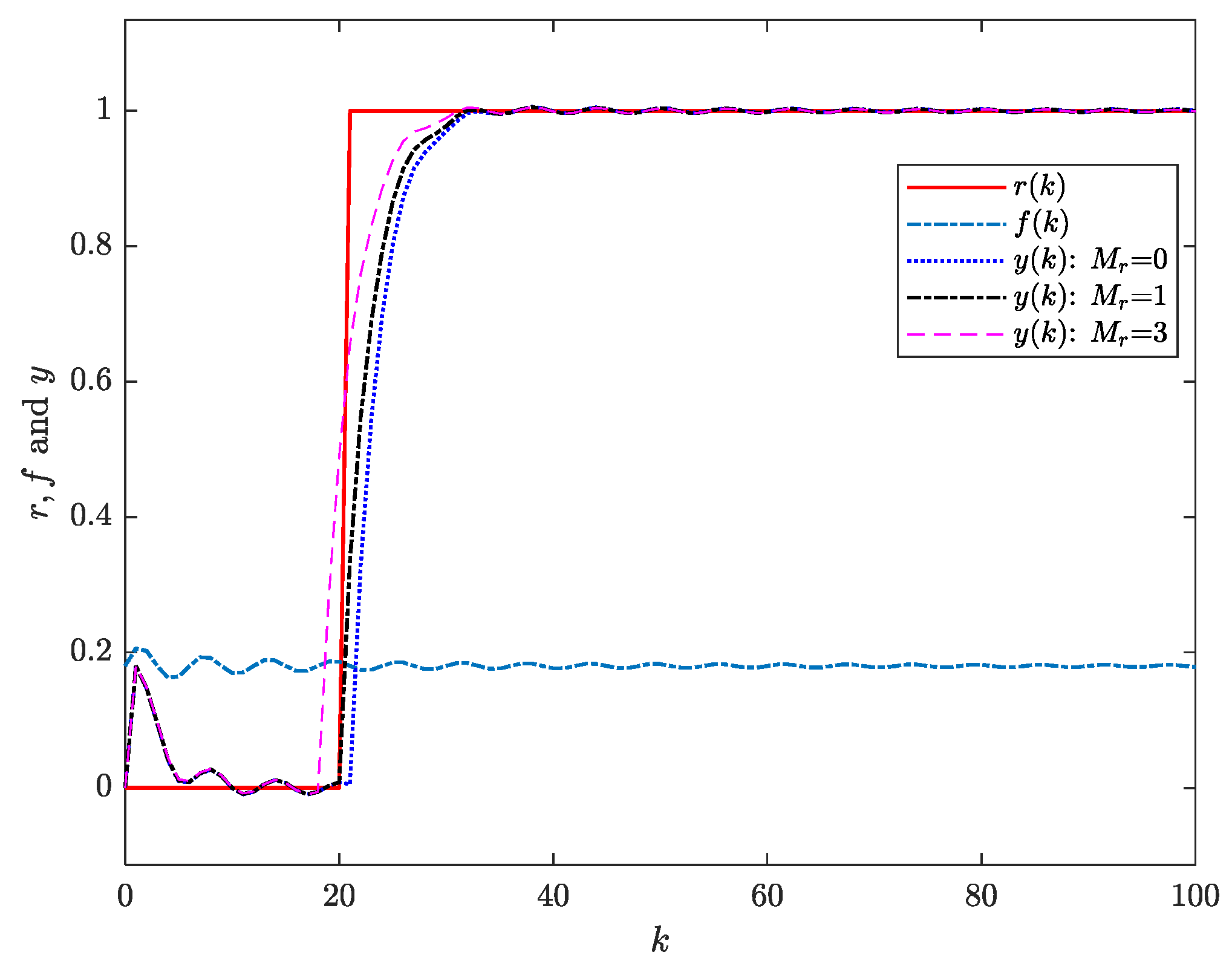
Example 1. 
As mentioned in the introduction, the discrete-time system corresponding to the pressurizer control system model is given by Equation (2). By setting the sampling interval as T = 0.1 , it follows from (2) and T s = 1 that the time delay τ = s 1 = 1 T 1 = 9 . The performance index function (5) is specified with weighting matrices Q e = 20 and H = 3 , while the disturbance attenuation level is set to γ = 6 . In system (2), the parameter p k + p 0 + p s is chosen as  0.18 sin ( π k / 3 ) k + 5 + 0.18 . The initial condition is x ( k ) = φ ( k ) = 0 , k 9 , 0 . We perform numerical simulations for two distinct reference signals.
(I) Step signal
r ( k ) = 0 ,               k 20 1 ,               k > 20
To investigate the effect of preview information on system performance, comparative simulations are performed for different preview lengths ( M r = 0 , M r = 1 and M r = 3 ). When M r = 0 , the matrices M = 0 20 0 0 0 0 , N = 0 3 . When M r = 1 , the matrices M = 0 20 0 0 0 0 0 0 , N = 0 3 . When M r = 3 , the matrices M = 0 20 0 0 0 0 0 0 0 0 0 0 , N = 0 3 .
The closed-loop output responses to the step reference signal (37) are shown in 
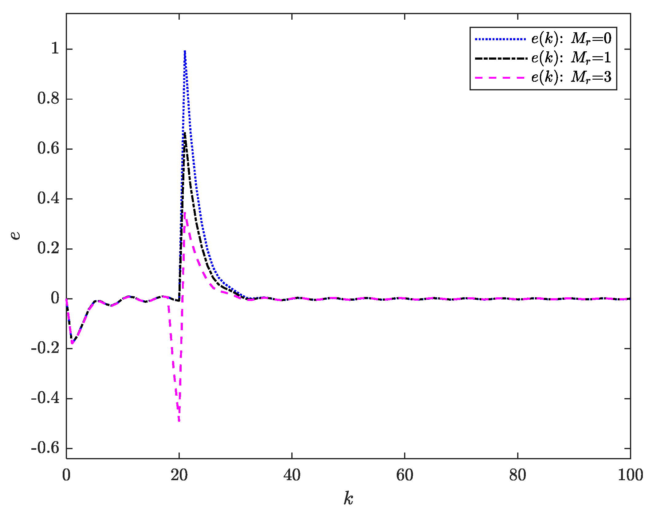
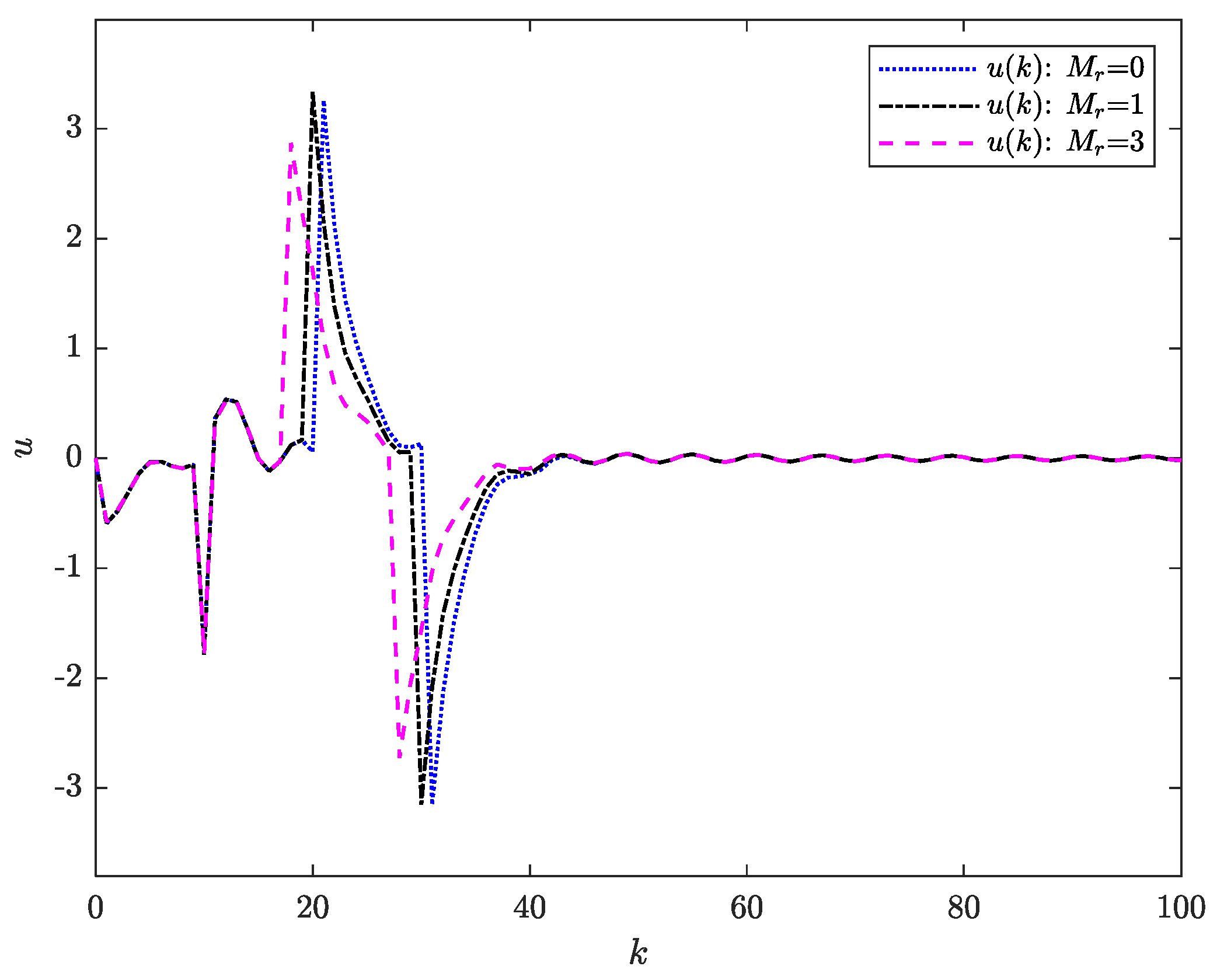
Figure 1. The corresponding tracking errors and control inputs are depicted in Figure 2 and Figure 3, respectively.
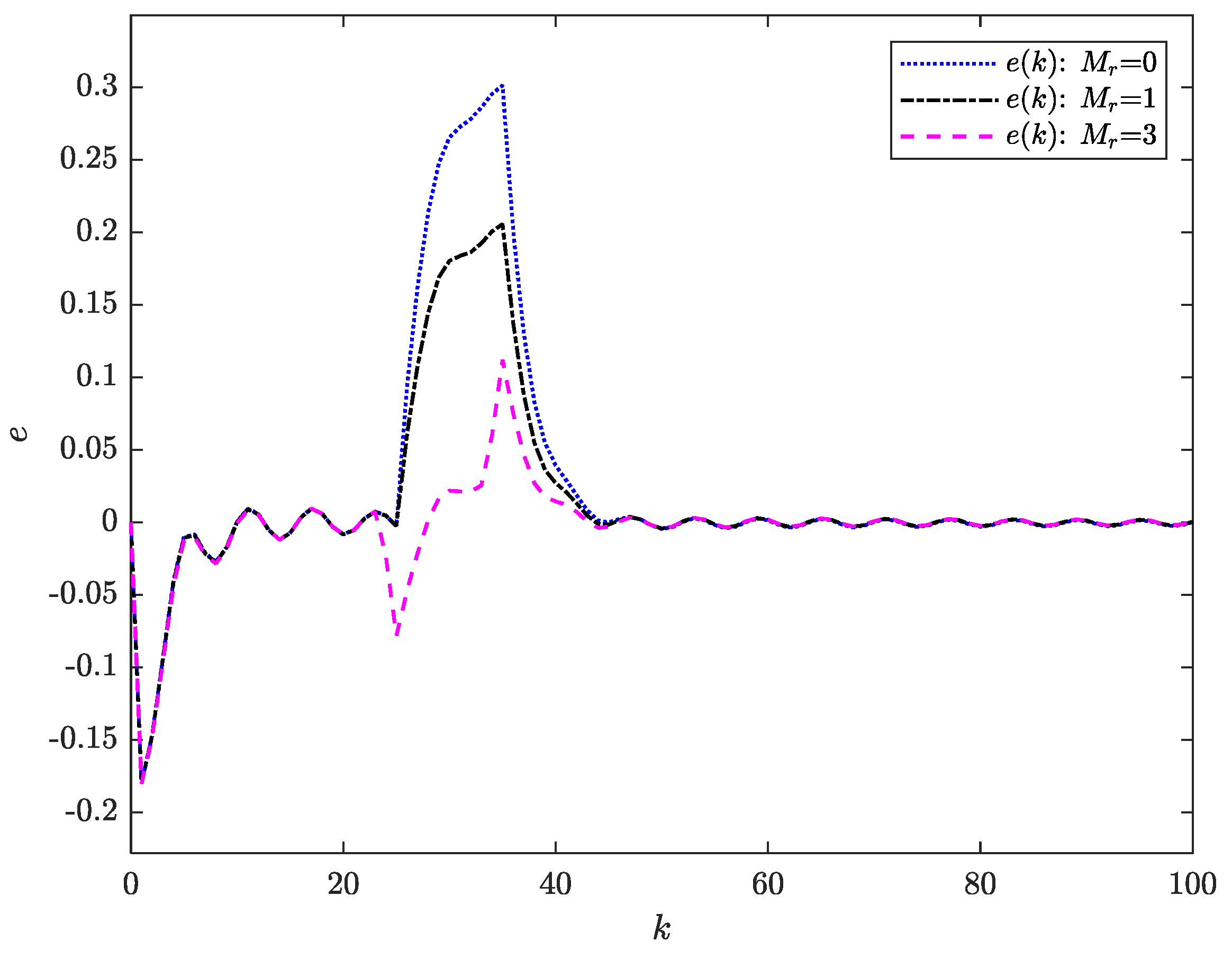
From Figure 1, it can be observed that the system output successfully tracks the reference signal under the three preview conditions ( M r = 0 , M r = 1 and M r = 3 ). Moreover, the preview-based controller enhances transient performance by accelerating the tracking speed. 
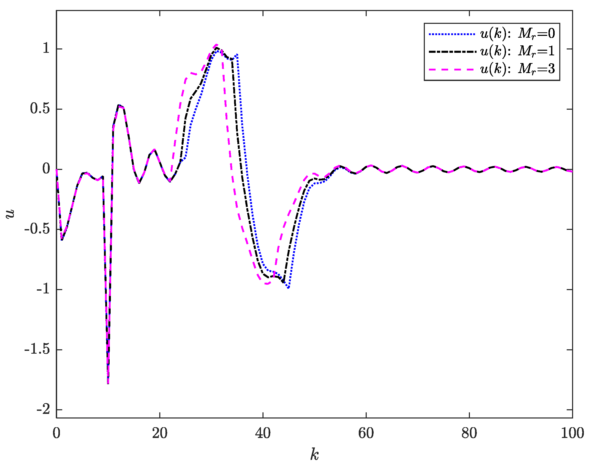
Figure 2 further reveals that the preview action contributes to a reduction in tracking error. As evidenced in Figure 3, the control input remains bounded across all preview horizons.
(I) Ramp signal
r ( k ) = 0 , k 25 0.1 ( k 25 ) , 25 < k 35 1 , k > 35
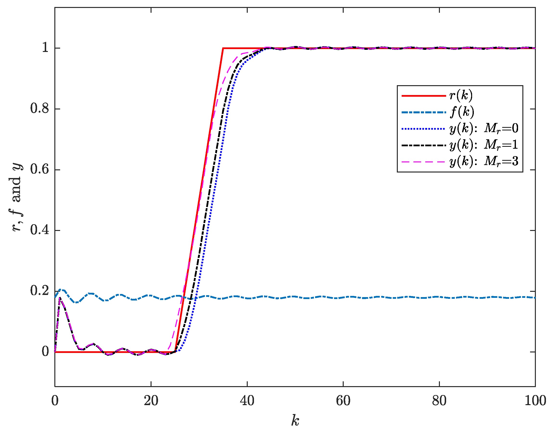
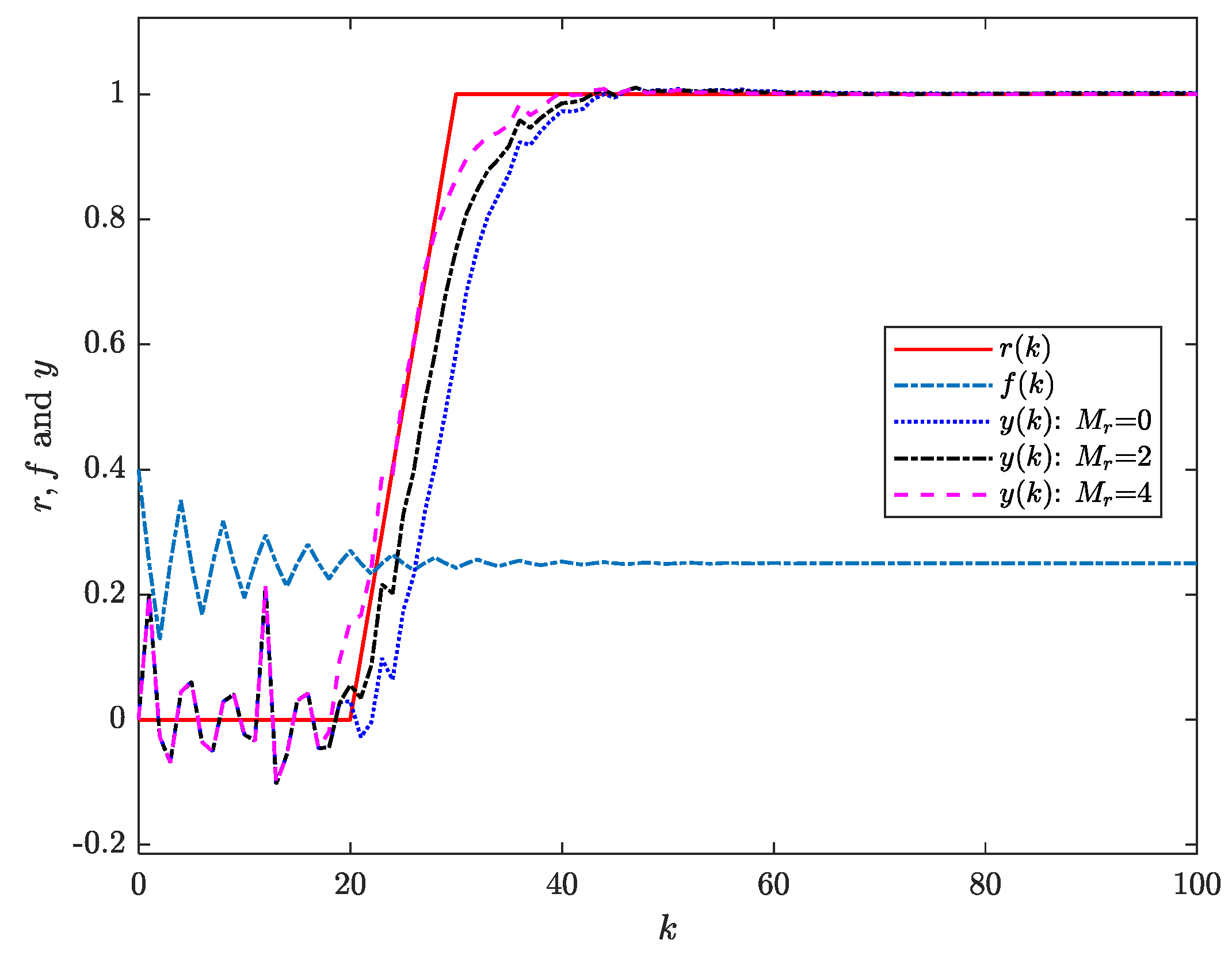
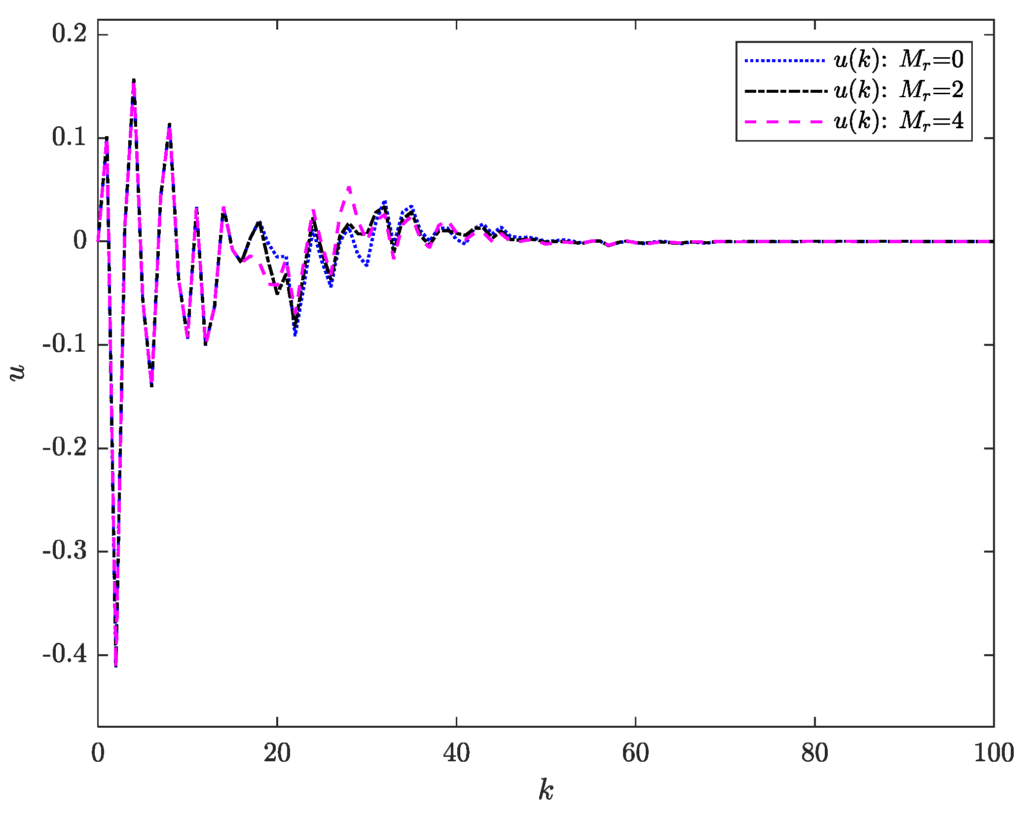
Similarly, in order to illustrate the influence of preview information on the closed-loop system, three cases of M r = 0 , M r = 1 and M r = 3 are simulated, respectively.
Figure 4, Figure 5 and 
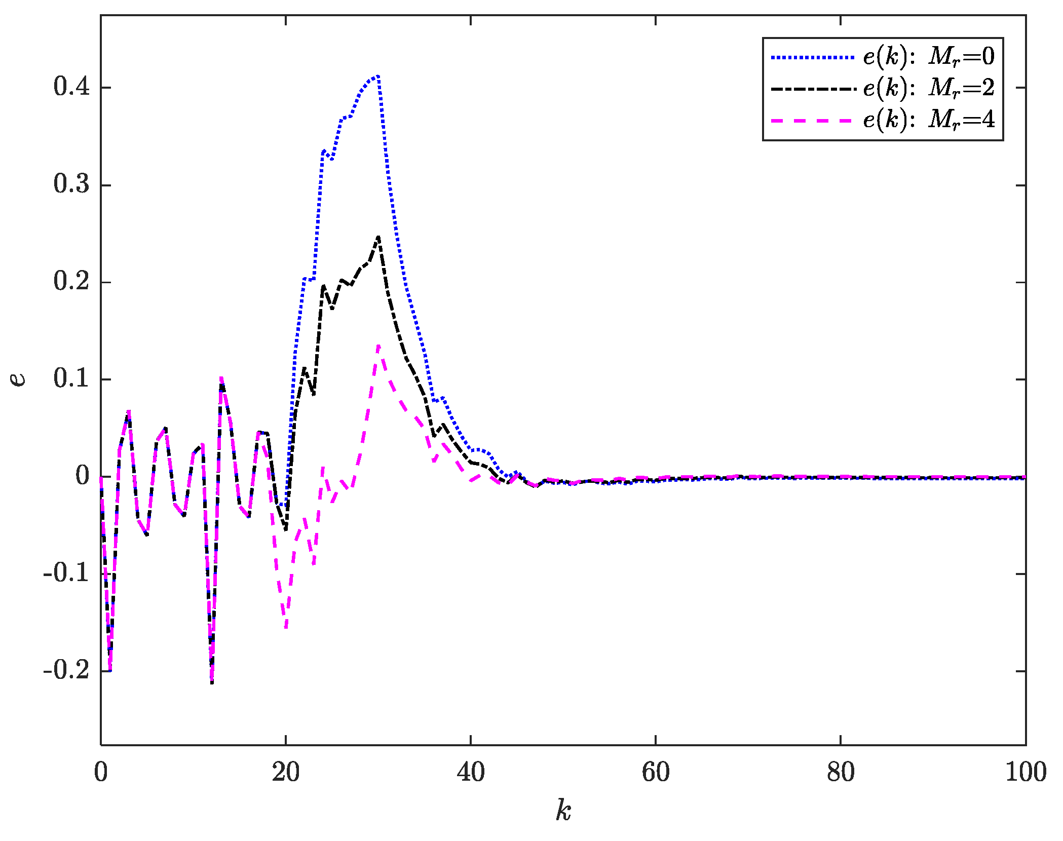
Figure 6 show the output response, tracking error, and control input of the closed-loop system, respectively. Similarly, it can be observed from Figure 4 and Figure 5 that as the preview horizon of the reference signal increases, the tracking error decreases, and the output of the closed-loop system follows the reference signal more quickly. Figure 6 demonstrates that the control input remains bounded.
Through numerical computation, we obtained the Integral of Absolute Error (IAE) and Integral of Time-weighted Absolute Error (ITAE) values for three preview step configurations: When M r = 0 , IAE = 3.7226 , ITAE = 110.5119 ; When M r = 1 , IAE = 2.7581 , ITAE = 78.2054 ; When M r = 3 , IAE = 1.3996 , ITAE = 32.659 . Moreover, to illustrate the impact of different weight matrix selections on the tracking performance of the system, we conducted simulations using various weight matrices and levels of disturbance attenuation. The corresponding IAE and ITAE values are calculated, and the results are summarized in Table 1.
In practical applications, these weights are typically chosen by control engineers based on specific performance requirements, such as prioritizing tracking accuracy, reducing control energy, or enhancing disturbance rejection.
Example 2. 
Consider the following discrete-time delay system
x 1 ( k + 1 ) x 2 ( k + 2 ) x 3 ( k + 3 ) = 1 0 0 0 0.5 1 0 0 1 A 1 x 1 ( k ) x 2 ( k ) x 3 ( k ) + 0 0.5 0 0 0 0.75 0 0.1 0.15 A 2 x 1 ( k 10 ) x 2 ( k 10 ) x 3 ( k 10 ) + 1 1 1 B [ u ( 0 ) + u ( 1 ) + + u ( k ) ] + 1 1 1 E f ( k ) y ( k ) = 0.5 1 0 C x 1 ( k ) x 2 ( k ) x 3 ( k )
and the external disturbance signal is
f ( k ) = 0.15 cos ( π k / 2 ) exp ( 0.1 k ) + 0.25 .
The reference signal is set as
r ( k ) = 0 , k 20 0.1 ( k 20 ) , 20 < k 30 1 , k > 30
Let the initial state function φ ( k ) be constant zero, and the weight matrix in the performance index function be Q e = 0.5 , H = 3 . Numerical simulations were conducted for three cases: no preview ( M r = 0 ), and preview steps M r = 2 and M r = 4 . Using MATLAB’s LMI toolbox, we obtain the following results:
when M r = 0 ,
K = 0.358252338651705 0.112061930141664 0.641758087309508 0.163320561923319 0 6.91412617895494 × 10 05 L = 2.39784847364747 × 10 09 0.220929746682905 0.230547051394449 1.57612529919375 × 10 08 0 1.03935716102284 × 10 08 γ = 3.65448750256443 ;
when M r = 2 ,
K = 0.357665257673321 0.111732194387077 0.642208708769576 0.161665089904687 0.161607051174762 0.171832900073115 6.60521899758945 × 10 05 L = 1.07791672721958 × 10 07 0.220737485245606 0.230363400531145 1.22728072265489 × 10 07 1.15456631304217 × 10 07 1.10868897390792 × 10 08 6.28914913419646 × 10 07 γ = 3.6554110451204 ;
when M r = 4 ,
K = 0.357959549065635 0.111954106814333 0.64199813087612 0.162694066716701 0.16256607057034                                                         0.172709317581974 0.204271083093631 0.171391028540036 0.000129917891651663 L = 5.26217449382389 × 10 08 0.220762550181414 0.230495994559622 5.37992176159413 × 10 08 3.28800302845288 × 10 08                                                         1.86325187434858 × 10 08 1.16115832288978 × 10 08 1.70893154224927 × 10 09 4.54499087027965 × 10 08 γ = 3.65521303687492 .
The tracking performance of system (39) is shown in Figure 7. From the figure, it can be observed that as time increases, the output signal of system (39) asymptotically tracks the reference signal, regardless of whether preview action is employed. By comparing the system responses under controllers with preview (i.e., M r = 2 or M r = 4 ) and without preview (i.e., M r = 0 ), it can be observed that the preview-based controllers enable the output vector to respond in advance and allow the system output to track the reference signal more rapidly. The tracking error of the system is shown in Figure 8. By examining Figure 7 and Figure 8 together, it can be observed that increasing the preview horizon improves the tracking accuracy, and the overall system error decreases as the preview horizon lengthens. Figure 9 shows the control input of the system. It can be seen from Figure 9 that the control input remains bounded. These findings verify the effectiveness of preview control in enhancing the system’s tracking performance.
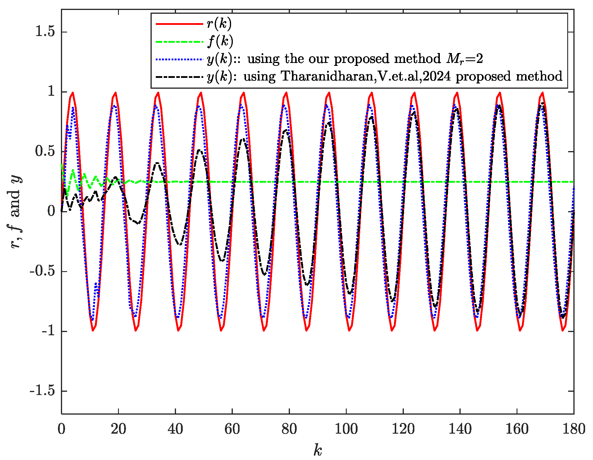
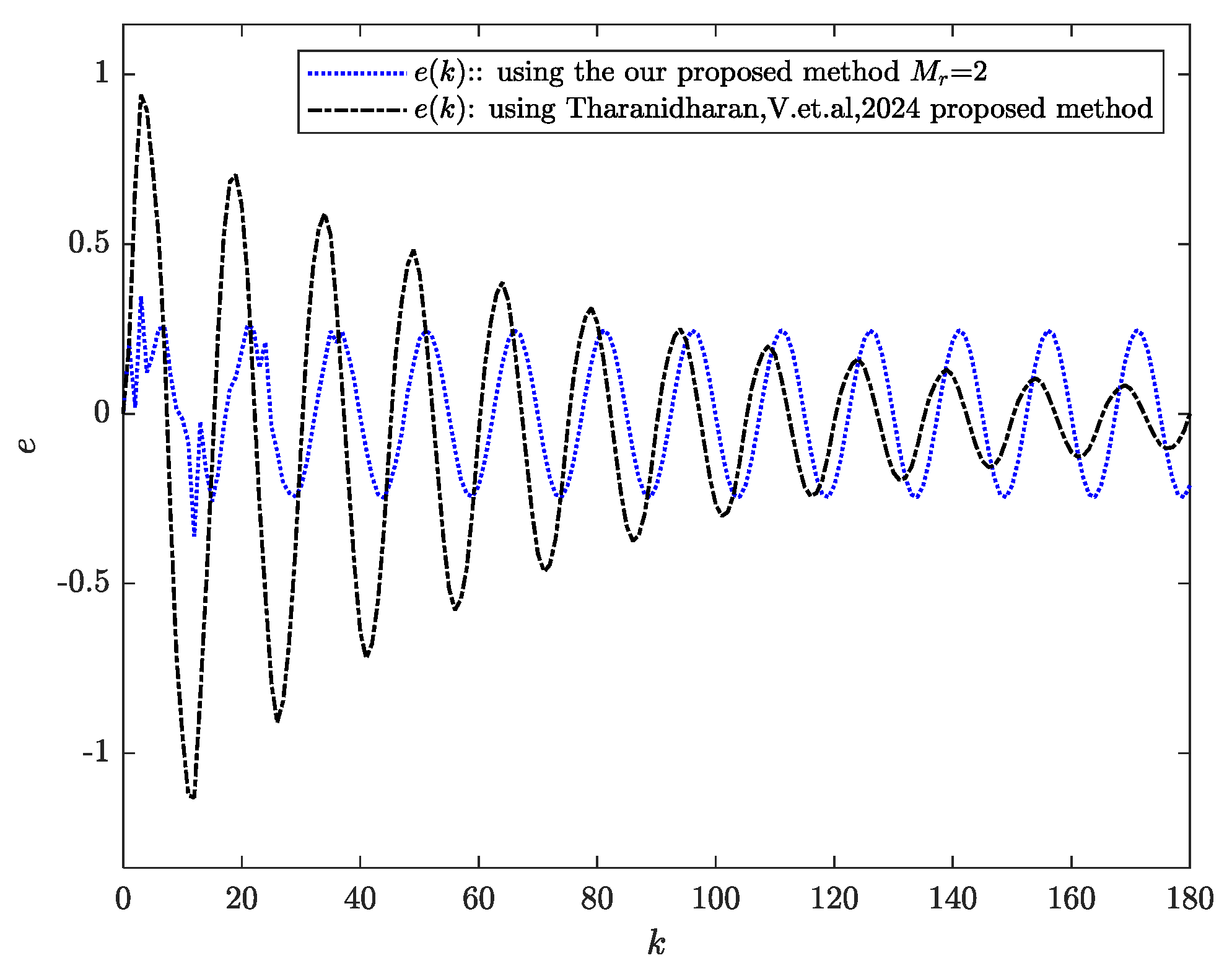
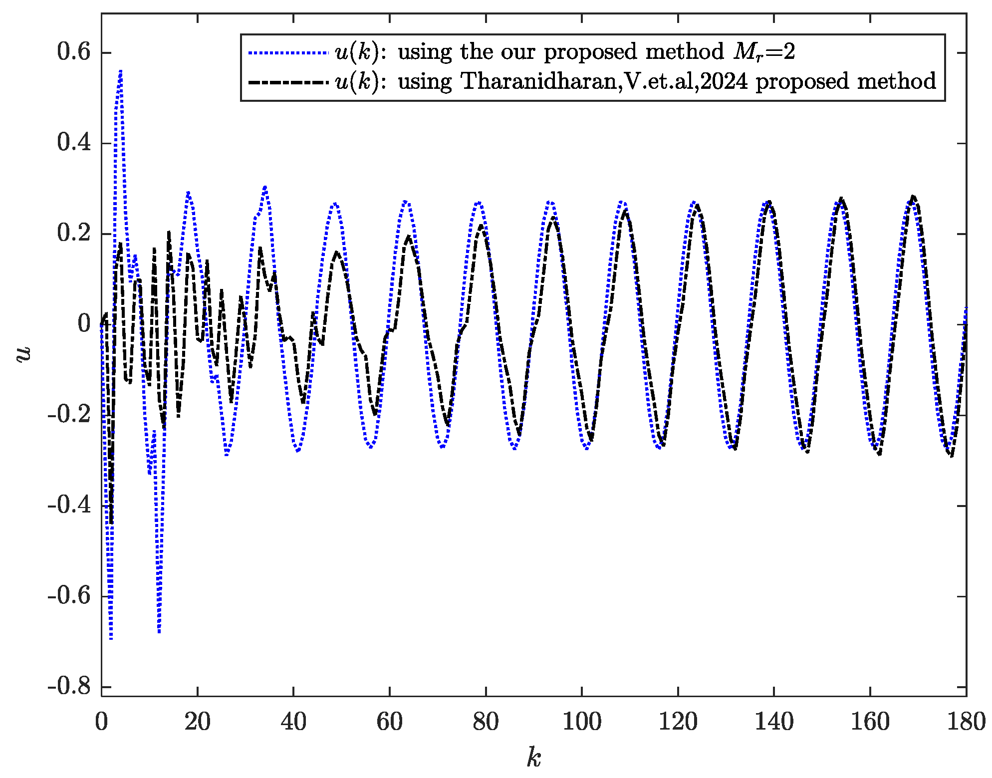
To enable a direct comparison between the proposed preview tracking control method and the repetitive tracking control method based on reference [32], we applied both approaches to simulate Example 2. Since repetitive tracking control is designed for periodic signal tracking, the reference signal was selected as: r ( k ) = sin 2 π k 15 . In addition, we set Q e = 5 , M r = 2 , γ = 8 , while keeping all other parameters the same as those in Example 2. The simulation results are shown in Figure 10, Figure 11 and Figure 12, where the black line represents the control method from reference [32], and the blue line corresponds to the proposed control method.
Through this comparison, we observed that for periodic signal tracking, the proposed preview-based method demonstrates significantly better performance during the initial tracking stage. However, as time progresses, the tracking error of the repetitive control method gradually becomes smaller than that of the preview-based approach. This indicates that both methods have their respective advantages: the preview control strategy offers a faster initial response, while the repetitive control method achieves better long-term steady-state accuracy.

6. Conclusions

This paper presents the design of an H preview tracking controller for a class of discrete-time systems with state delays, originating from the nuclear reactor pressurizer control system. The studied system in this paper differs from conventional control systems in that its control inputs consist of the cumulative sum of historical inputs. The main objective of this work is to develop a preview tracking controller for such an unconventional system. By applying the difference method and state augmentation approach, an augmented error system was constructed to include both the reference signal and a discrete-time integrator. A performance signal was accordingly defined, and the preview tracking control problem was reformulated as an H control problem. A conventional Lyapunov function was utilized to derive stability conditions in the form of linear matrix inequalities, leading to a transparent and rigorous derivation of the proposed controller. The obtained controller was then successfully applied to the simplified nuclear reactor pressurizer system. Numerical simulations demonstrated that increasing the preview step significantly improves the closed-loop tracking performance, validating the effectiveness of the proposed method.
It is worth mentioning that the considered system is a simplified model, and potential uncertainties and nonlinearities have not been accounted for. As part of our future research, we aim to explore the application of preview control to more realistic pressurizer models and address the challenges posed by system uncertainties and nonlinearities. Furthermore, adopting more advanced Lyapunov functions could potentially reduce conservatism in the controller design, and this will also be an important direction for our future investigations.

Author Contributions

Conceptualization, investigation, F.L.; methodology, writing, F.L. and H.X.; software, formal analysis, H.X., X.M., and J.W.; writing—review and editing, validation, J.W., Y.W. and J.D. All authors have read and agreed to the published version of the manuscript.

Funding

This work was funded by the National Natural Science Foundation of China with grant number 61174209, the Scientific Research Project of Hechi University with grant number 2020XJYB001, the High-level Talent Research Start-up Project of Chongqing Technology and Business University with grant number 2356029, and the Engineering and Physical Sciences Research Council (EPSRC) of UK with grant numbers EP/R021961/1.

Data Availability Statement

Data are contained within the article.

Conflicts of Interest

The authors declare no conflicts of interest.

References

  1. Birla, N.; Swarup, A. Optimal preview control: A review. Optim. Control Appl. Methods 2015, 36, 241–268. [Google Scholar] [CrossRef]
  2. Yu, X.; Lu, R.H.; Yuan, Y.L. Reliable preview tracking control for a class of discrete-time Lipschitz nonlinear systems. J. Syst. Sci. Math. Sci. 2023, 43, 2804–2819. [Google Scholar]
  3. Xie, H.; Liao, F.; Ge, S.S. Robust preview control of interconnected continuous-time systems with parametric uncertainties. Appl. Math. Model. 2023, 118, 107–127. [Google Scholar] [CrossRef]
  4. Wu, J.; Liao, F.; Xu, Z. Preview control for a class of linear stochastic systems with multiplicative noise. Int. J. Syst. Sci. 2019, 50, 2592–2603. [Google Scholar] [CrossRef]
  5. Lan, Y.H.; Zhao, J.Y.; She, J.H. Preview repetitive control with equivalent input disturbance for continuous-time linear systems. IET Control Theory Appl. 2022, 16, 125–138. [Google Scholar] [CrossRef]
  6. Han, K.; Feng, J. Data-driven robust fault tolerant linear quadratic preview control of discrete-time linear systems with completely unknown dynamics. Int. J. Control 2021, 94, 49–59. [Google Scholar] [CrossRef]
  7. Li, L.; Lu, Y.R.; Song, S.Y. Preview saturated control for uncertain periodic discrete-time systems. J. Syst. Sci. Math. Sci. 2024, 44, 99–114. [Google Scholar]
  8. Sheridan, T.B. Three models of preview control. IEEE Trans. Hum. Factors Electron. 1966, 7, 91–102. [Google Scholar] [CrossRef]
  9. Itoh, H.; Tsuchiya, T. Introducing virtual axis to path control system using superficial evaluation term. JSME Int. J. 1996, 39, 815–821. [Google Scholar] [CrossRef]
  10. Abe, S.; Tsuchiya, T. Robot manipulator path control based on variable speed trajectory planning. Adv. Robot. 1991, 6, 1–13. [Google Scholar] [CrossRef]
  11. Youn, I.; Ahmad, E. Anti-jerk optimal preview control strategy to enhance performance of active and semi-active suspension systems. Electronics 2022, 11, 1657. [Google Scholar] [CrossRef]
  12. Choi, H.D.; Lee, C.J.; Lim, M.T. Fuzzy preview control for half-vehicle electro-hydraulic suspension system. Int. J. Control Autom. Syst. 2018, 16, 2489–2500. [Google Scholar] [CrossRef]
  13. Tong, X.; Zhao, X. Vibration and power regulation control of a floating wind turbine with hydrostatic transmission. Renew. Energy 2021, 167, 899–906. [Google Scholar] [CrossRef]
  14. Guo, F.; Schlipf, D.; Zhang, Z.; Cheng, P.W. Investigation on the wind preview quality for lidar-assisted wind turbine control under wake conditions. In Proceedings of the 2022 American Control Conference, Atlanta, GA, USA, 8–10 June 2022; pp. 3544–3549. [Google Scholar]
  15. Huang, Y.; Luo, W.; Lan, H. Adaptive pre-aim control of driverless vehicle path tracking based on a SSA-BP neural network. World Electr. Veh. J. 2022, 13, 55. [Google Scholar] [CrossRef]
  16. Zhang, Y.D.; Wang, Q.Y.; Liu, Q.Q.; Ji, Y.; Xu, M. Optimal preview tracking control algorithm for ATO system. J. Comput. Appl. 2017, 37, 266–269. [Google Scholar]
  17. Xue, Y.; Chen, Y.; Tao, C.; Zou, Y.; Zhen, Z. Disturbance rejection based on discrete-time adaptive preview control for unmanned aerial vehicle shipboard landing under structure damage. Proc. Inst. Mech. Eng. Part I-J. Syst. Control Eng. 2024, 238, 1102–1111. [Google Scholar] [CrossRef]
  18. Yan, C.Q. Nuclear Reactor Engineering, 3rd ed.; Harbin Engineering University Press: Harbin, China, 2020. [Google Scholar]
  19. Gu, Z. History review of nuclear reactor safety. Ann. Nucl. Energy 2018, 120, 682–690. [Google Scholar] [CrossRef]
  20. Zhang, G.Z.; Yang, X.H.; Lu, D.Q.; Liu, Y. Research on water level and pressure control system of nuclear reactor regulator. Control Instrum. Chem. Ind. 2013, 40, 35–42. [Google Scholar]
  21. Cui, C.; Zhang, J.; Shen, J. System-level modeling, analysis and coordinated control design for the pressurized water reactor nuclear power system. Energy 2023, 283, 128472. [Google Scholar] [CrossRef]
  22. Wei, H.; Zhu, N.; Sun, Z.; Tan, S.; Tian, R. Research on the intelligent control strategy of pressurizer pressure in PWRs based on a fuzzy neural network PID controller. Nucl. Eng. Des. 2025, 433, 113875. [Google Scholar] [CrossRef]
  23. Xue, Y.; Lin, J.; Li, Y.; Feng, J.B. Research on pressurizer water level control in nuclear reactor based on active disturbances rejection controller. Appl. Mech. Mater. 2013, 336, 608–613. [Google Scholar] [CrossRef]
  24. Luan, Z.; Wang, M.; Zhang, Y.; Wei, Q.; Zhou, T.; Guo, Z.; Ling, J. Optimal Tracking Control for a Discrete Time Nonlinear Nuclear Power System. Math. Probl. Eng. 2022, 2022, 7953358. [Google Scholar] [CrossRef]
  25. Naimi, A.; Deng, J.; Vajpayee, V.; Becerra, V.; Shimjith, S.R.; Arul, A.J. Nonlinear model predictive control using feedback linearization for a pressurized water nuclear power plant. IEEE Access 2022, 10, 16544–16555. [Google Scholar] [CrossRef]
  26. Brown, C.; Gabbar, H.A. Fuzzy logic control for improved pressurizer systems in nuclear power plants. Ann. Nucl. Energy 2014, 72, 461–466. [Google Scholar] [CrossRef]
  27. Mydlo, P.; Schreiber, P. Fuzzy controller for the control of nuclear reactor’s power-control rods. In Proceedings of the 22nd Central European Conference on Information and Intelligent Systems, Dubrovnik, Croatia, 20–22 September 2011. [Google Scholar]
  28. Wang, M.; Deng, J.; Pattinson, C.; Richardson, S. A fuzzy controller for fault tolerant control of nuclear reactor. In Proceedings of the 2017 International Conference on Computational Science and Computational Intelligence, Las Vegas, NV, USA, 14–16 December 2017; pp. 387–390. [Google Scholar]
  29. Katayama, T.; Ohki, T.; Inoue, T.; Kato, T. Design of an optimal controller for a discrete-time system subject to previewable demand. Int. J. Control 1985, 41, 677–699. [Google Scholar] [CrossRef]
  30. Yu, L. Robust Control: Linear Matrix Inequality Approach; Tsinghua University Press: Pekin, China, 2002. [Google Scholar]
  31. Yung, C.F.; Wang, C.C.; Wu, P.F.; Wang, H.S. Bounded real lemma for linear discrete-time descriptor systems. IFAC Proc. 2008, 41, 9982–9986. [Google Scholar] [CrossRef]
  32. Tharanidharan, V.; Saravanakumar, T.; Anthoni, S.M. Robust and quantized repetitive tracking control for fractional-order fuzzy large-scale systems. Int. J. Adapt. Control Signal Process. 2024, 38, 1496–1511. [Google Scholar] [CrossRef]
Figure 1. Output response of the closed−loop system tracking the step reference signal (37).
Axioms 14 00505 g001
Figure 2. Tracking error of the closed−loop system for the step reference signal (37).
Axioms 14 00505 g002
Figure 3. Control input of the closed−loop system tracking the step reference signal (37).
Axioms 14 00505 g003
Figure 4. Output response of the closed−loop system tracking the step reference signal (38).
Axioms 14 00505 g004
Figure 5. Tracking error of the closed−loop system for the step reference signal (38).
Axioms 14 00505 g005
Figure 6. Control input of the closed−loop system tracking the step reference signal (38).
Axioms 14 00505 g006
Figure 7. The output response of system (39).
Axioms 14 00505 g007
Figure 8. Tracking error of system (39).
Axioms 14 00505 g008
Figure 9. Control input of system (39).
Axioms 14 00505 g009
Figure 10. Output of the systems using the proposed method and Tharanidharan, V. et al., 2024 [32].
Axioms 14 00505 g010
Figure 11. Tracking errors using the proposed method and Tharanidharan, V. et al., 2024 [32].
Axioms 14 00505 g011
Figure 12. Input of the systems using the proposed method and Tharanidharan, V. et al., 2024 [32].
Axioms 14 00505 g012
Table 1. IAE and ITAE under different weight combinations.
Different Weight CombinationsIAEITAE
Q e = 20 , H = 3 , γ = 9 , M r = 3 1.955352.717
Q e = 30 , H = 3 , γ = 9 , M r = 3 1.428235.781
Q e = 20 , H = 6 , γ = 9 , M r = 4 1.899145.1989
Q e = 20 , H = 3 , γ = 5 , M r = 5 2.163253.4079
Disclaimer/Publisher’s Note: The statements, opinions and data contained in all publications are solely those of the individual author(s) and contributor(s) and not of MDPI and/or the editor(s). MDPI and/or the editor(s) disclaim responsibility for any injury to people or property resulting from any ideas, methods, instructions or products referred to in the content.

