
LDC-GAT: A Lyapunov-Stable Graph Attention Network with Dynamic Filtering and Constraint-Aware Optimization


Abstract
1. Introduction
1.1. Related Work
1.2. Our Approach
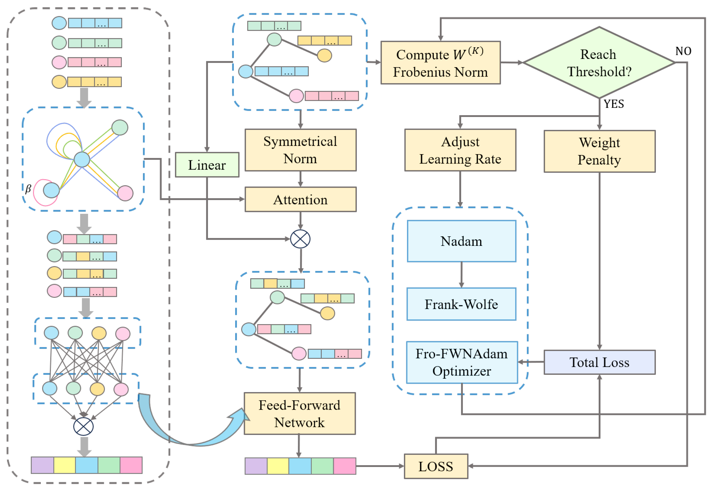
- We introduce Dynamic Residual Graph Filtering (DRG-Filtering), where a tunable self-loop factor dynamically regulates the coupling between neighborhood and self-node features. Moreover, we refer to the energy conservation idea of the Hamiltonian graph dynamics model [24] to construct a DRG-Filtering that maintains the Dirichlet energy lower bound.
- We derive a Frobenius norm constraint for multi-head attention weights using Lyapunov theory, which is subsequently used to design the learning-rate-aware perceptron. This strategy dynamically gauges the compatibility between the current learning rate and local loss landscape characteristics by computing the relative relationship between the Frobenius norm of the weight matrix and a predefined critical threshold.
- We pioneer the design of a projection-free optimization algorithm FWNAdam by integrating the Nesterov momentum mechanism into the Frank–Wolfe framework. By replacing high-dimensional projection steps with linear searches, and embedding the proposed learning-rate-aware perceptron into FWNAdam, we introduce Fro-FWNAdam, which ensures feasibility under convex constraints while enabling progressively stable network optimization.
2. Preliminaries
2.1. Graph Attention Networks
2.2. Dirichlet Energy and Graph Filtering
2.3. Lyapunov Stability in Discrete Dynamical Systems
2.4. Regret Bounds
3. Dynamic Residual Graph Filtering
4. The Frobenius Norm Constraints for Multi-Head Weights
5. Optimization Under Norm Constraints: The Fro-FWNAdam Algorithm
6. LDC-GAT
| Algorithm 1 Fro-FWNAdam |
| Require: , adjacency matrix A, step size , initial parameters , norm threshold , contraction rate Ensure: Updated parameters , feature matrix , learning rates
|
7. Simulations
8. Conclusions
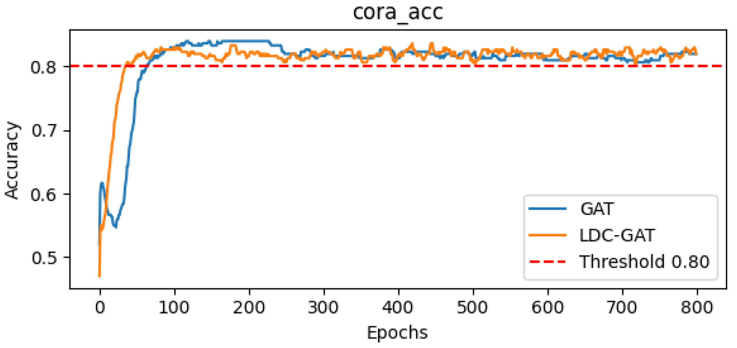
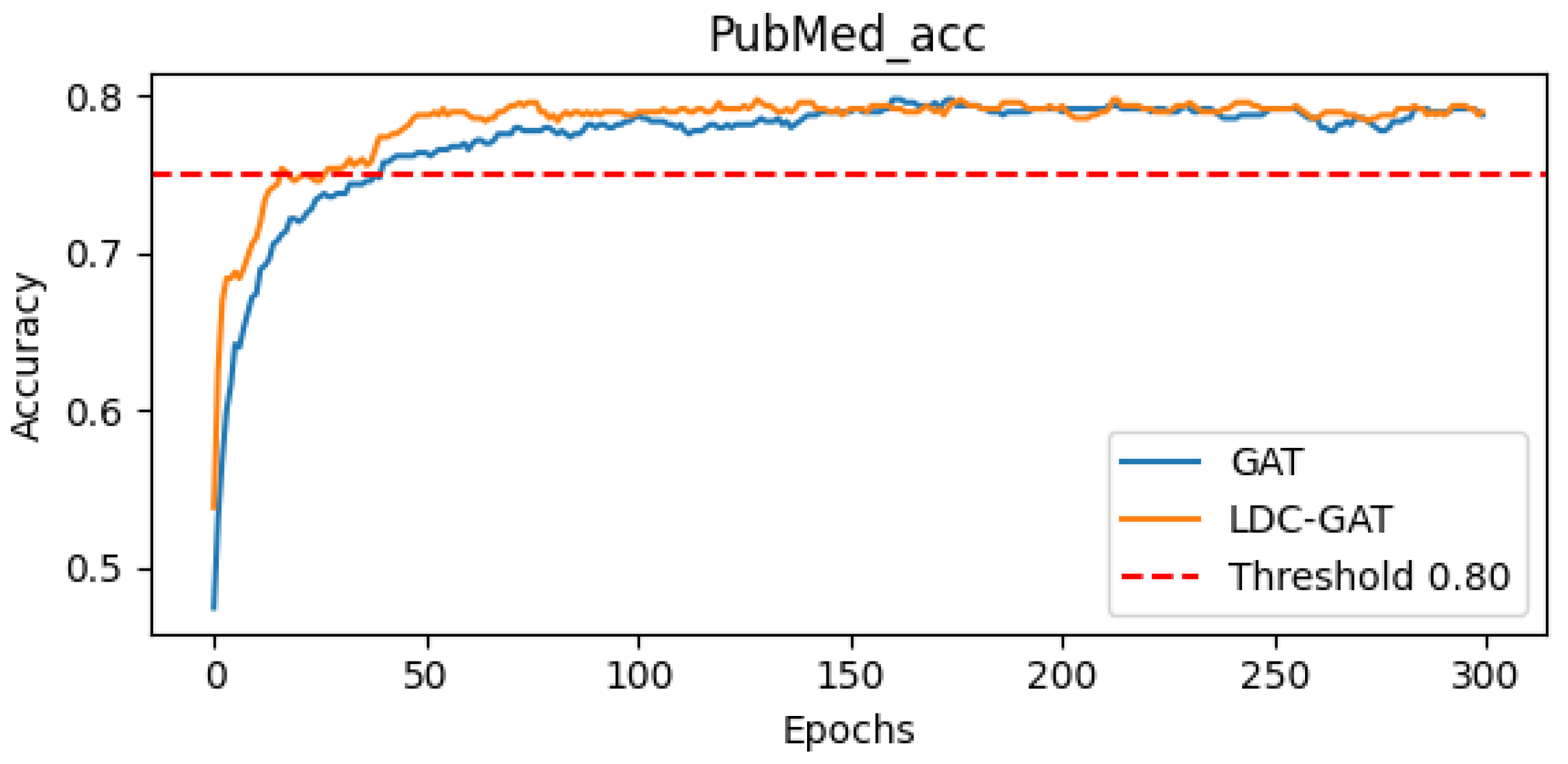
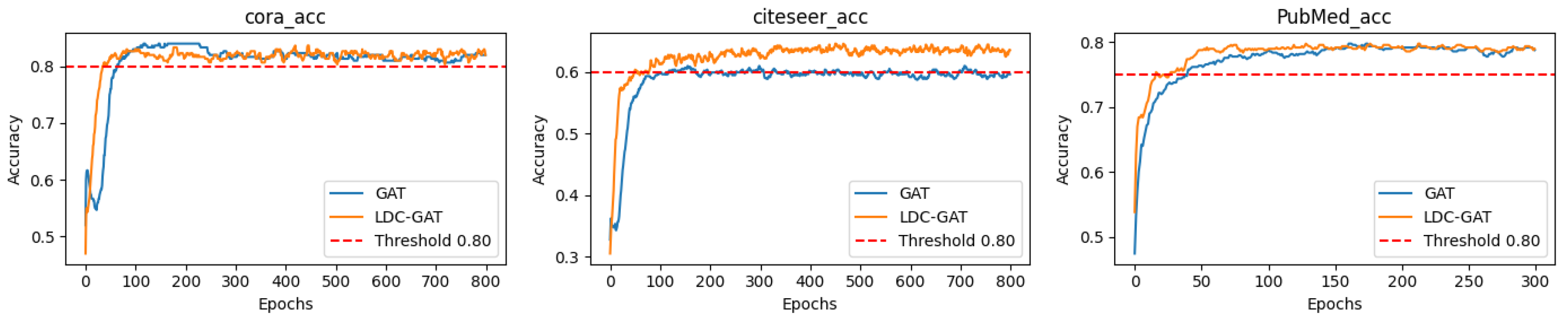
- In semi-supervised classification tasks, LDC-GAT demonstrates an average accuracy improvement of approximately 10.54% over vanilla GAT across six benchmark datasets (including Cora and PubMed), validating the effectiveness of multi-band signal fusion enabled by its dynamic residual filtering mechanism for cross-layer feature injection.
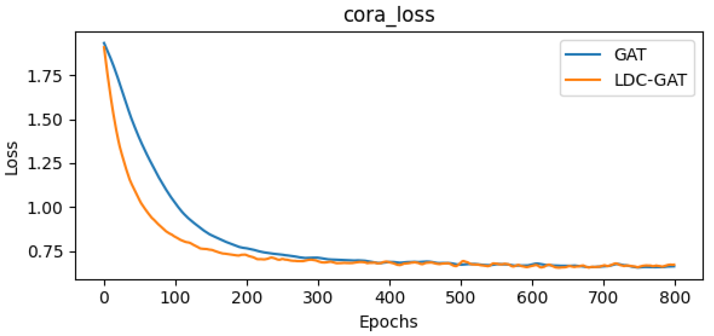
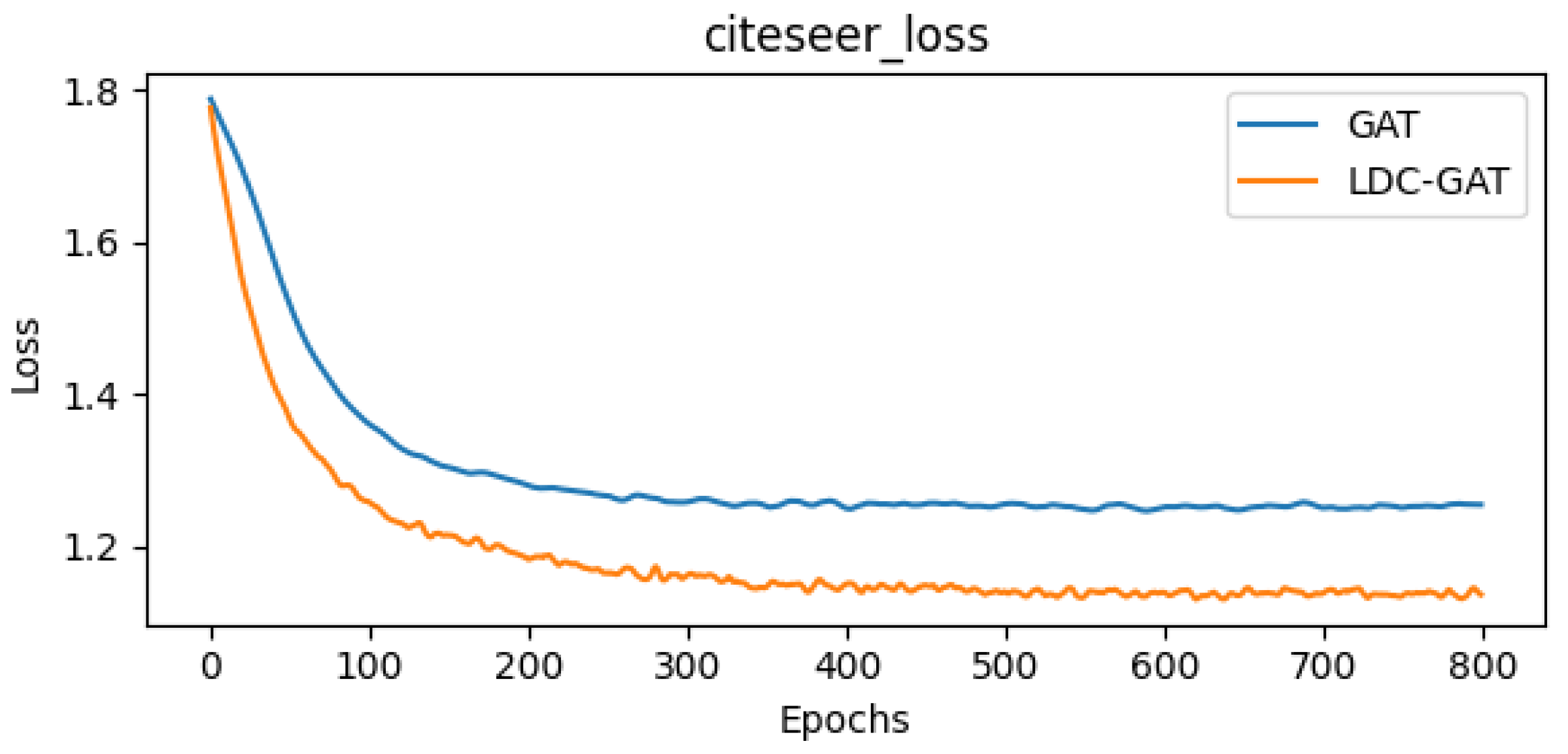
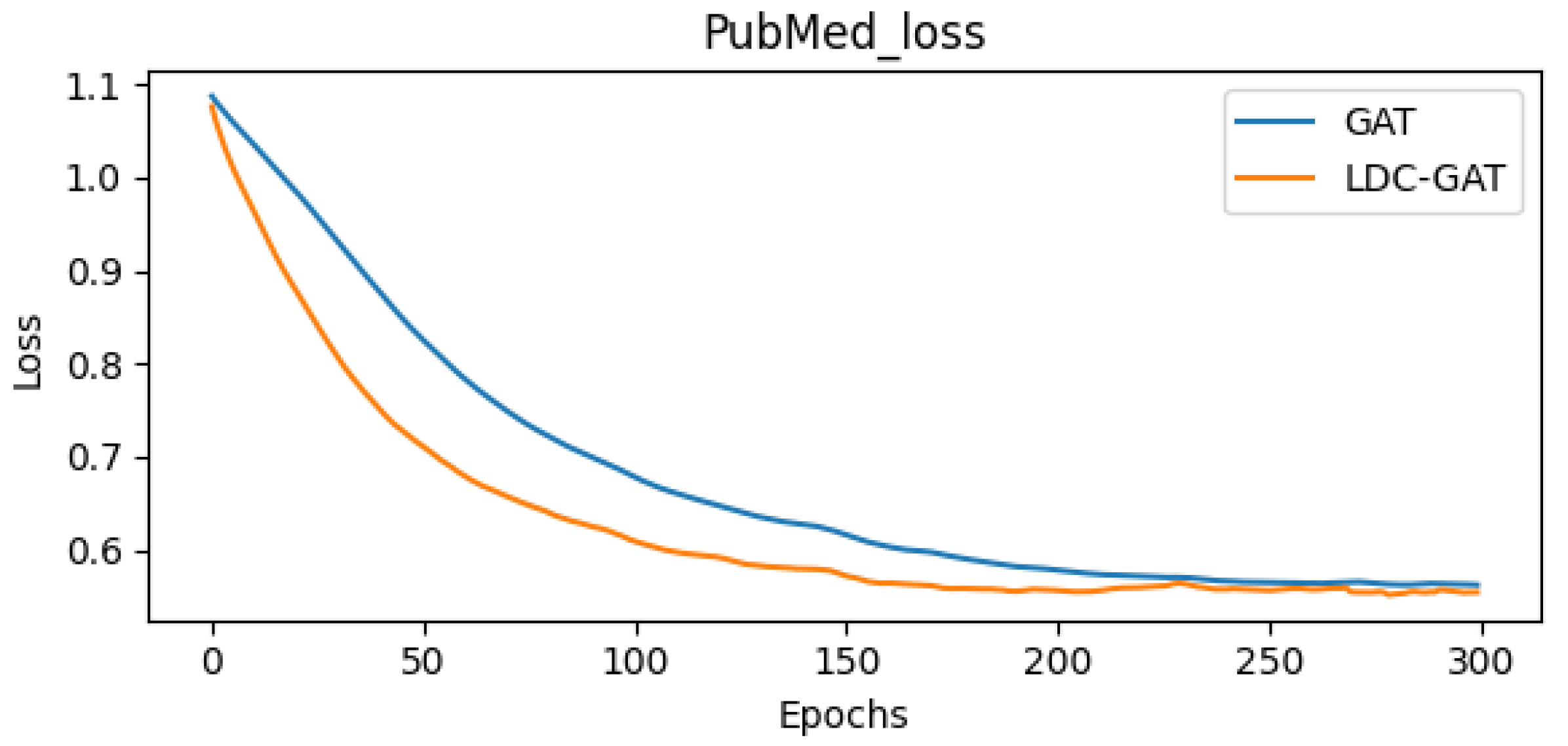
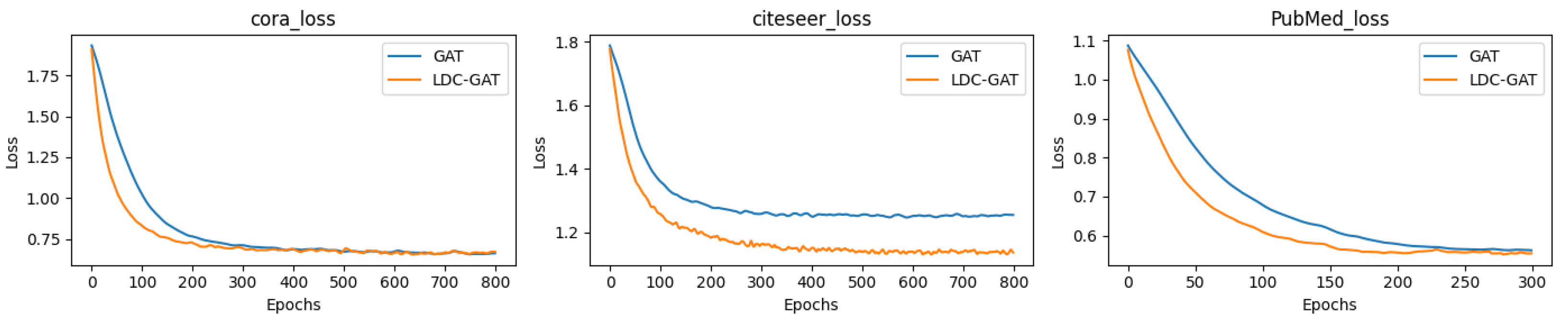
- For constrained optimization, LDC-GAT pioneers explicit parameter-space compression through Frobenius norm constraint boundaries on multi-head weight matrices. The proposed collaborative optimization algorithm, Fro-FWNAdam, integrates dynamic learning rate adaptation, Nesterov momentum acceleration, and Frank–Wolfe direction search. It improves convergence speed by 10.6% while ensuring constraint feasibility, making it well suited for constrained scenarios.
Author Contributions
Funding
Data Availability Statement
Conflicts of Interest
Appendix A. Proof of Theorem 1
Appendix B. Poof of Lemma 1
Appendix C. Poof of Theorem 2
Appendix D. Detailed Presentation of Subfigures in Figure 2 and Figure 3
References
- Grover, A.; Leskovec, J. node2vec: Scalable feature learning for networks. In Proceedings of the 22nd ACM SIGKDD International Conference on Knowledge Discovery and Data Mining, San Francisco, CA, USA, 13–17 August 2016; pp. 855–864. [Google Scholar]
- Gilmer, J.; Schoenholz, S.S.; Riley, P.F.; Vinyals, O.; Dahl, G.E. Neural message passing for quantum chemistry. In Proceedings of the 34th International Conference on Machine Learning, Sydney, Australia, 6–11 August 2017; pp. 1263–1272. [Google Scholar]
- Bruna, J.; Zaremba, W.; Szlam, A.; LeCun, Y. Spectral networks and locally connected networks on graphs. arXiv 2013, arXiv:1312.6203. [Google Scholar]
- Veličković, P.; Cucurull, G.; Casanova, A.; Romero, A.; Liò, P.; Bengio, Y. Graph attention networks. In Proceedings of the International Conference on Learning Representations, Vancouver, BC, Canada, 30 April–3 May 2018. [Google Scholar]
- Defferrard, M.; Bresson, X.; Vandergheynst, P. Convolutional neural networks on graphs with fast localized spectral filtering. In Advances in Neural Information Processing Systems 29; Curran Associates: Barcelona, Spain, 2016; pp. 3844–3852. [Google Scholar]
- Li, Q.; Han, Z.; Wu, X.-M. Deeper insights into graph convolutional networks for semi-supervised learning. In Proceedings of the Thirty-Second AAAI Conference on Artificial Intelligence, New Orleans, LA, USA, 2–7 February 2018; pp. 3538–3545. [Google Scholar]
- He, K.; Zhang, X.; Ren, S.; Sun, J. Deep residual learning for image recognition. In Proceedings of the IEEE Conference on Computer Vision and Pattern Recognition, Las Vegas, NV, USA, 27–30 June 2016; pp. 770–778. [Google Scholar]
- Kipf, T.N.; Welling, M. Semi-supervised classification with graph convolutional networks. In Proceedings of the International Conference on Learning Representations, Toulon, France, 24–26 April 2017. [Google Scholar]
- Oono, K.; Suzuki, T. Graph neural networks exponentially lose expressive power for node classification. In Proceedings of the International Conference on Learning Representations, Addis Ababa, Ethiopia, 26–30 April 2020. [Google Scholar]
- Pareja, A.; Domeniconi, G.; Chen, J.; Ma, T.; Suzumura, T.; Kanezashi, H.; Kaler, T. EvolveGCN: Evolving graph convolutional networks for dynamic graphs. In Proceedings of the Thirty-Fourth AAAI Conference on Artificial Intelligence, New York, NY, USA, 7–12 February 2020; pp. 5363–5370. [Google Scholar]
- Bronstein, M.M.; Bruna, J.; LeCun, Y.; Szlam, A.; Vandergheynst, P. Geometric deep learning: Going beyond Euclidean data. IEEE Signal Process. Mag. 2017, 34, 18–42. [Google Scholar] [CrossRef]
- Balcilar, M.; Héroux, P.; Gaüizère, B.; Taminato, R.J.; Vazirgiannis, M.; Malliaros, F.D. Breaking the limits of message passing graph neural networks. In Proceedings of the 38th International Conference on Machine Learning, Virtual Event, 18–24 July 2021; pp. 599–608. [Google Scholar]
- Xu, K.; Hu, W.; Leskovec, J.; Jegelka, S. How powerful are graph neural networks? In Proceedings of the International Conference on Learning Representations, New Orleans, LA, USA, 6–9 May 2019. [Google Scholar]
- Newman, M.E.J. Mixing patterns in networks. Phys. Rev. E 2003, 67, 026126. [Google Scholar] [CrossRef] [PubMed]
- He, W.; Wei, Z.; Huang, Z.; Li, J.; Li, H. BerNet: Learning arbitrary graph spectral filters via Bernstein approximation. In Proceedings of the 35th Conference on Neural Information Processing Systems (NeurIPS), Virtual Event, 6–14 December 2021. [Google Scholar]
- Chen, D.; Lin, Y.; Li, W.; Li, P.; Zhou, J.; Sun, X. Stability and generalization of graph convolutional neural networks. In Proceedings of the 28th ACM SIGKDD Conference on Knowledge Discovery and Data Mining, Washington, DC, USA, 14–18 August 2022; pp. 1539–1547. [Google Scholar]
- Kingma, D.P.; Ba, J. Adam: A method for stochastic optimization. In Proceedings of the International Conference on Learning Representations, San Diego, CA, USA, 7–9 May 2015. [Google Scholar]
- McCallum, A.K.; Nigam, K.; Rennie, J.; Seymore, K. Automating the construction of internet portals with machine learning. In Proceedings of the 17th International Conference on Machine Learning, Stanford, CA, USA, 29 June–2 July 2000; pp. 327–334. [Google Scholar]
- Kim, Y.; Lee, S.; Kim, J.; Park, J. Stabilizing multi-head attention in transformers through gradient regularization. In Proceedings of the 36th Conference on Neural Information Processing Systems (NeurIPS), New Orleans, LA, USA, 28 November–9 December 2022. [Google Scholar]
- Lv, S.; Shen, Y.; Qian, H.; Li, Y.; Wang, X. Robust graph neural networks under distribution shifts: A causal invariance approach. In Proceedings of the 40th International Conference on Machine Learning, Honolulu, HI, USA, 23–29 July 2023. [Google Scholar]
- Kavis, M.J.; Xu, Z.; Goldfarb, D. Projection-free adaptive methods for constrained deep learning. J. Mach. Learn. Res. 2023, 24, 1–38. [Google Scholar]
- Ngo, T.; Yin, J.; Ge, Y.-F.; Wang, H. Optimizing IoT intrusion detection—A graph neural network approach with attribute-based graph construction. Information 2025, 16, 499. [Google Scholar] [CrossRef]
- Chen, L.; Zhu, H.; Han, S. Stability-optimized graph convolutional network: A novel propagation rule with constraints derived from ODEs. Mathematics 2025, 13, 761. [Google Scholar] [CrossRef]
- Hamilton, W.L.; Ying, R.; Leskovec, J. Inductive representation learning on large graphs. In Proceedings of the Advances in Neural Information Processing Systems 30, Long Beach, CA, USA, 4–9 December 2017; pp. 1024–1034. [Google Scholar]
- Tan, C.W.; Yu, P.-D.; Chen, S.; Poor, H.V. DeepTrace: Learning to optimize contact tracing in epidemic networks with graph neural networks. IEEE Trans. Signal Inf. Process. Netw. 2025, 11, 97–113. [Google Scholar] [CrossRef]
- Shah, D.; Zaman, T. Rumors in a network: Who’s the culprit? IEEE Trans. Inf. Theory 2011, 57, 5163–5181. [Google Scholar] [CrossRef]
- Yan, J.; Duan, Y. Momentum cosine similarity gradient optimization for graph convolutional networks. Comput. Eng. Appl. 2024, 60, 133–143. [Google Scholar]
- Gama, F.; Bruna, J.; Ribeiro, A. Stability properties of graph neural networks. IEEE Trans. Signal Process. 2019, 68, 5680–5695. [Google Scholar] [CrossRef]
- Zhang, M.; Zhou, Y.; Quan, W.; Wang, Y.; Zhao, Q. Online learning for IoT optimization: A Frank–Wolfe Adam-based algorithm. IEEE Internet Things J. 2020, 7, 8228–8237. [Google Scholar] [CrossRef]
- Chang, B.; Chen, M.; Haber, E.; Chi, E.H. AntisymmetricRNN: A dynamical system view on recurrent neural networks. arXiv 2019, arXiv:1902.09689. [Google Scholar]
- Pei, H.; Wei, B.; Chang, K.C.-C.; Lei, Y.; Yang, B. Geom-GCN: Geometric graph convolutional networks. arXiv 2020, arXiv:2002.05287. [Google Scholar]
- Bo, D. Research on Key Technologies of Spectral Domain Graph Neural Networks. Ph.D. Thesis, Beijing University of Posts and Telecommunications, Beijing, China, 2023. [Google Scholar]

| Dataset | Nodes | Edges | Classes | Features | Homophily Level |
|---|---|---|---|---|---|
| Cora | 2708 | 5429 | 7 | 1433 | 0.81 |
| Citeseer | 3327 | 4732 | 6 | 3703 | 0.74 |
| PubMed | 19,717 | 44,338 | 3 | 500 | 0.80 |
| Chameleon | 2277 | 36,101 | 3 | 2325 | 0.18 |
| Texas | 183 | 309 | 5 | 1703 | 0.11 |
| Squirrel | 5201 | 217,073 | 3 | 2089 | 0.018 |
| DRG-Filtering | Weight Norm Constraints | Fro-FWNAdam | Acc | Loss |
|---|---|---|---|---|
| × | × | × | 83.90% | 1.0893 |
| ✓ | × | × | 83.94% | 1.0725 |
| ✓ | ✓ | × | 84.28% | 1.0549 |
| ✓ | ✓ | ✓ | 84.50% | 1.0433 |
| DRG-Filtering | Weight Norm Constraints | Fro-FWNAdam | Acc | Loss |
|---|---|---|---|---|
| × | × | × | 60.31% | 1.2416 |
| ✓ | × | × | 63.14% | 1.1317 |
| ✓ | ✓ | × | 65.74% | 1.0288 |
| ✓ | ✓ | ✓ | 67.79% | 0.9677 |
| Metric | Cora | Citeseer | PubMed |
|---|---|---|---|
| GAT mean accuracy | 83.90% | 48.75% | 77.70% |
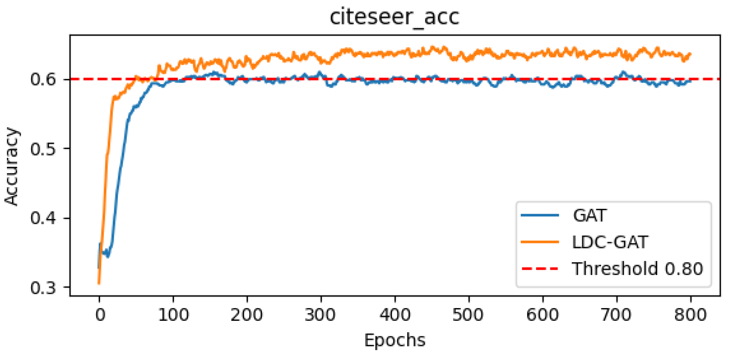
| LDC-GAT mean accuracy | 84.50% | 54.45% | 78.20% |
| Standard deviation (±) | ±0.0031 | ±0.0042 | ±0.0045 |
| Confidence interval (95%) | [84.2%, 84.8%] | [53.9%, 55.0%] | [78.0%, 78.4%] |
| p-value | 0.011 | 0.002 | 0.025 |
| Metric | Chameleon | Texas | Squirrel |
|---|---|---|---|
| GAT mean accuracy | 60.31% | 60.31% | 42.65% |
| LDC-GAT mean accuracy | 67.79% | 81.88% | 70.13% |
| Standard deviation (±) | ±0.0050 | ±0.0020 | ±0.0050 |
| Confidence interval (95%) | [67.4%, 68.2%] | [81.6%, 82.1%] | [69.8%, 70.5%] |
| p-value | 0.0005 | 0.0001 | 0.0012 |
| Homophilic Graph Datasets | Heterophilic Graph Datasets | |||||
|---|---|---|---|---|---|---|
| Model | Cora | Citeseer | PubMed | Chameleon | Texas | Squirrel |
| Graph SAGE | 78.00 | 52.19 | 76.00 | 66.67 | 56.76 | 56.20 |
| MLP | 57.00 | 53.35 | 72.90 | 50.44 | 78.38 | 42.56 |
| ChebNet | 73.60 | 53.85 | 69.00 | 58.77 | 81.78 | 39.75 |
| GCN | 83.60 | 50.23 | 77.90 | 47.55 | 37.84 | 69.80 |
| GIN | 76.40 | 47.60 | 77.00 | 66.89 | 56.75 | 52.16 |
| GAT | 83.90 | 48.75 | 77.70 | 61.31 | 60.31 | 42.65 |
| LDC-GAT | 84.50 | 54.45 | 78.20 | 67.79 | 81.88 | 70.13 |
| Edge Removal Ratio | Drop 10% | Drop 30% | Drop 50% | |||
|---|---|---|---|---|---|---|
| Model | GAT | LDC-GAT | GAT | LDC-GAT | GAT | LDC-GAT |
| Cora | 83.1 | 83.6 | 78.6 | 81.9 | 76.6 | 79.6 |
| Citeseer | 46.17 | 52.79 | 45.38 | 51.89 | 44.13 | 51.42 |
| PubMed | 75.2 | 77.92 | 72.3 | 75.68 | 71.8 | 75.2 |
| Chameleon | 59.65 | 66.94 | 59.64 | 66.91 | 59.36 | 65.8 |
| Squirrel | 40.46 | 70.08 | 40.25 | 69.88 | 39.88 | 69.7 |
| Texas | 57.76 | 79.76 | 56.76 | 78.46 | 54.05 | 76.05 |
Disclaimer/Publisher’s Note: The statements, opinions and data contained in all publications are solely those of the individual author(s) and contributor(s) and not of MDPI and/or the editor(s). MDPI and/or the editor(s) disclaim responsibility for any injury to people or property resulting from any ideas, methods, instructions or products referred to in the content. |
© 2025 by the authors. Licensee MDPI, Basel, Switzerland. This article is an open access article distributed under the terms and conditions of the Creative Commons Attribution (CC BY) license (https://creativecommons.org/licenses/by/4.0/).
Share and Cite
Chen, L.; Zhu, H.; Han, S. LDC-GAT: A Lyapunov-Stable Graph Attention Network with Dynamic Filtering and Constraint-Aware Optimization. Axioms 2025, 14, 504. https://doi.org/10.3390/axioms14070504
Chen L, Zhu H, Han S. LDC-GAT: A Lyapunov-Stable Graph Attention Network with Dynamic Filtering and Constraint-Aware Optimization. Axioms. 2025; 14(7):504. https://doi.org/10.3390/axioms14070504
Chicago/Turabian StyleChen, Liping, Hongji Zhu, and Shuguang Han. 2025. "LDC-GAT: A Lyapunov-Stable Graph Attention Network with Dynamic Filtering and Constraint-Aware Optimization" Axioms 14, no. 7: 504. https://doi.org/10.3390/axioms14070504
APA StyleChen, L., Zhu, H., & Han, S. (2025). LDC-GAT: A Lyapunov-Stable Graph Attention Network with Dynamic Filtering and Constraint-Aware Optimization. Axioms, 14(7), 504. https://doi.org/10.3390/axioms14070504